Development of a Compensation Scheme for a Measurement Voltage Transformer Using the Hysteresis Characteristics of a Core

Abstract

This paper describes the design, evaluation, and implementation of a compensation scheme for a measurement voltage transformer (VT) using the hysteresis characteristics of the core. The error of a VT is caused by the primary winding voltage and secondary winding voltage. The latter depends on the secondary current, whereas the former depends on the primary current, which is an aggregate of the exciting and secondary currents. The secondary current is obtained directly from the secondary voltage and is used to obtain the voltage across the secondary winding. For the primary current, the exciting current is decomposed into two components: core-loss and magnetizing currents. The magnetizing current is obtained by the flux-magnetizing current curve instead of the hysteresis loop to minimize the required loops for compensation. The core-loss current is obtained by dividing the primary induced voltage by the core-loss resistance. Finally, the estimated voltages across the primary and secondary windings are added to the measured secondary voltage for compensation. The scheme can significantly improve the accuracy of a VT. The results of the performance of compensator are shown in the experimental test. The accuracy of the measurement VT improves from 1.0C class to 0.1C class. The scheme can help to significantly reduce the required core cross section of a measurement VT in an electrical energy system.

1. Introduction

A voltage transformer (VT) is used to convert a high voltage in an electrical energy system into a low voltage signal. The secondary voltage of a VT is then fed into the metering device or the protection device. Both measurement VTs [1,2] and protection VTs [1,3] should meet the standard defined by IEC and IEEE. For a measuring VT, the IEC standard stipulates four accuracy classes of the rated voltage: 1.0C, 0.5C, 0.2C, and 0.1C at voltages of 80%, 100%, and 120%, respectively. The VT should satisfy both the ratio error and the phase error specified at each accuracy class. A 1.0C class VT is usually used only for measurement, while a VT higher than the 0.5C class is used for revenue.

So far, iron cores have been widely used in instrument transformers to maximize the mutual flux between the primary and secondary windings. However, the iron core has nonlinear hysteresis characteristics, which cause a non-sinusoidal exciting current.

The error of a VT results from the voltages across the primary and secondary winding impedances, while the error of a current transformer (CT) is caused by the exciting current. The voltage across the secondary winding impedance depends on the secondary current, while the voltage across the primary winding impedance depends on the primary current, which is the sum of the exciting and secondary currents. Therefore, both the exciting and secondary currents must be kept as small as possible to obtain the high accuracy needed for a VT.

Generally, the secondary current can be kept small by using a large burden of a VT. On the other hand, a large magnetizing inductance of the core is required in order to minimize the exciting current. The magnetizing inductance of the core depends on the permeability and geometry of the core. Therefore, to get the high accuracy of a VT, we need a core with high permeability and/or a large core cross section. However, this increases the size and cost of a measurement VT.

To obtain a highly accurate VT, compensation methods for the voltages across the primary and secondary windings have been proposed [4,5]. The total voltage of the primary and secondary windings was compensated [4], while the individual voltages across the primary and secondary windings were compensated [5]. The result of the method in [5] is better than that of [4]. However, the methods require additional circuitry for compensation, and did not consider the hysteresis characteristics of the core.

This paper proposes a compensation scheme for a measurement VT in the time domain using the hysteresis characteristics of the core. The proposed scheme estimates and compensates the primary and secondary winding voltages considering the effect of the hysteresis characteristics of the core. To do this, the primary and secondary currents should be estimated. The secondary current is obtained directly from the measured secondary voltage and is used to calculate the secondary winding voltage. The primary current consists of the secondary and exciting currents. The exciting current can be estimated by inserting the flux into the hysteresis loop. In this paper, the flux-magnetizing current (λ-i_m) curve is used instead of the hysteresis loop to minimize the required number of curves for interpolation. The core-loss current is determined by dividing the primary induced voltage by the core-loss resistance. The magnetizing current corresponding to the flux is obtained by inserting the flux into the λ-i_m curve. Finally, the estimated voltages across the primary and secondary windings are aggregated to the measured secondary voltage for compensation. The performance of the scheme was investigated with a 22.9 kV distribution system using an EMTP simulator. To validate the compensation scheme of the measurement VT, a digital signal processor (DSP) is investigated. This paper concludes by describing the results of experimental test of a prototype compensator based on a DSP.

2. Proposed Compensation Scheme of a Measurement VT

As mentioned in the Introduction, the estimation of the exciting current of the core is essential for VT compensation as well as for CT compensation. If we used the hysteresis curves of the core for compensation, interpolation for minimizing the number of required curves is required between the two contiguous curves. However, there is a limitation to reduce the number of required curves, because the hysteresis curves have quite different shapes, from 80% of the rated voltage to 120% of the rated voltage. For CT compensation, the exciting current was decomposed into the core-loss current and magnetizing currents and the λ-i_m curve was used to estimate the latter, instead of the hysteresis curve [6]. This contributes to significantly reduce the number of curves required for compensation because the λ-i_m curves have very similar patterns over the wide region of the current. Afterwards, we will describe the proposed compensation scheme for a measurement VT to improve the accuracy, which uses the λ-i_m curve instead of the hysteresis curve as in [6].

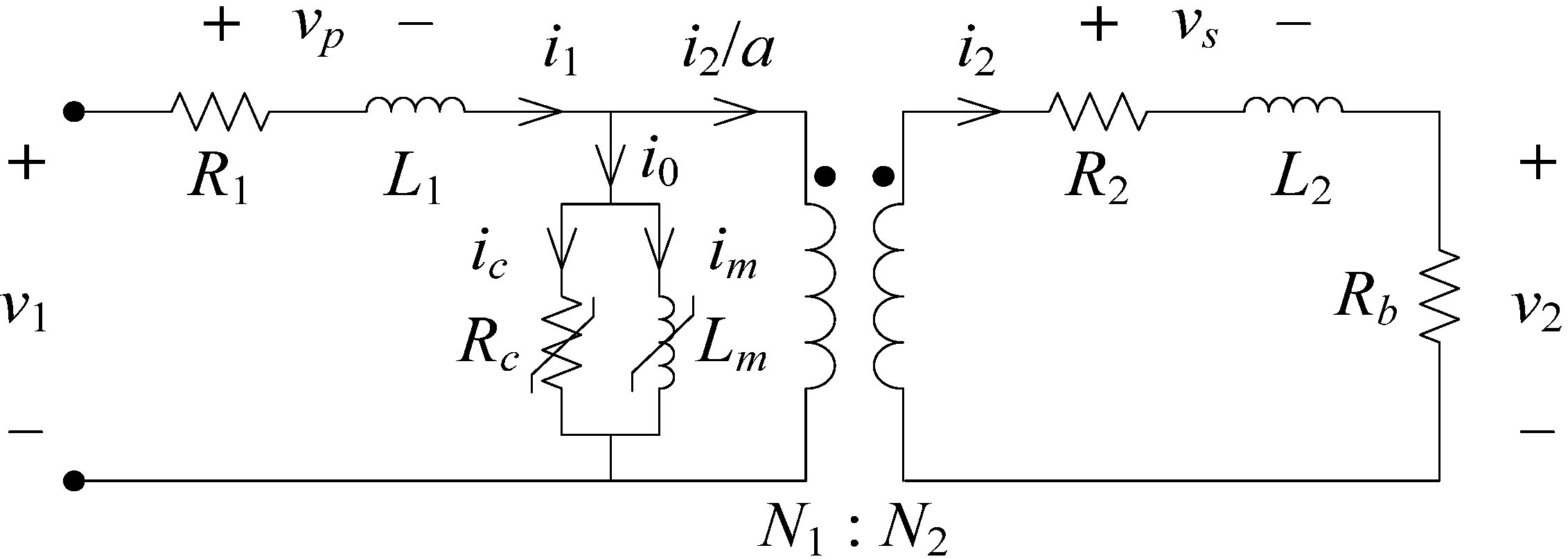
2.1. Equivalent Circuit of a VT

Figure 1 shows an equivalent circuit of an iron-cored VT. The hysteresis characteristics of the core are represented by the parallel connection of the core-loss resistance (R_c) and the magnetizing inductance (L_m).

Figure 1. Equivalent circuit of the VT. v₁, v₂: primary and secondary voltages; v_p, v_s: primary and secondary winding voltages; i₁, i₂: primary and secondary currents; i₀, i_c, i_m: exciting, core-loss, and magnetizing currents; R₁, L₁: primary winding parameters; R₂, L₂: secondary winding parameters; R_c, R_b,: core-loss and burden resistances; L_m: magnetizing inductance; N₁, N₂: primary and secondary windings; a=N₁/N₂: turns ratio.

Figure 1. Equivalent circuit of the VT. v₁, v₂: primary and secondary voltages; v_p, v_s: primary and secondary winding voltages; i₁, i₂: primary and secondary currents; i₀, i_c, i_m: exciting, core-loss, and magnetizing currents; R₁, L₁: primary winding parameters; R₂, L₂: secondary winding parameters; R_c, R_b,: core-loss and burden resistances; L_m: magnetizing inductance; N₁, N₂: primary and secondary windings; a=N₁/N₂: turns ratio.

L_m represents the nonlinear relationship between the flux linkage (λ) and i_m. R_c, which represents the sum of the eddy current loss and the hysteresis loss [7], is also nonlinear between v₂ and i_c. The relationship between v₁ and v₂ at any instant is given by:

$$v_1\left(t\right)=v_p\left(t\right)+a\left[v_s\right(t)+v_2(t\left)\right]$$

(1)

where a is the turns ratio (N₁/N₂).

In Equation (1), v_p + av_s causes the error of a VT. Thus, if v_p + av_s can be estimated at any instant, the error can be eliminated by adding the estimated v_p + av_s to the measured av₂. The procedure of estimating v_p and v_s will be explained in the following subsection.

2.2. Proposed Compensation Scheme of a VT

2.2.1. Secondary Winding Voltage (v_s)

The relationship between v_s and i₂ is given by:

$$v_s(t)=R_2{i}_2(t)+L_2\frac{d{i}_2\left(t\right)}{dt}$$

(2)

To calculate v_s, i₂ must be known, and can be obtained by:

$$i_2(t)=\frac{v_2\left(t\right)}{R_b}$$

(3)

Thus, v_s can be calculated by applying i₂ to Equation (2).

2.2.2. Primary Winding Voltage (v_p)

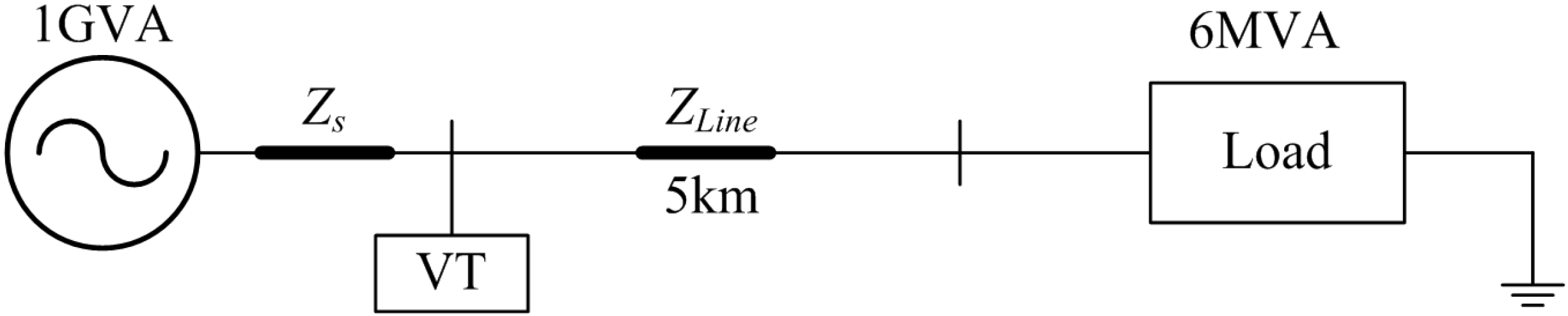
The relationship between v_p and i₁ can be expressed by:

$$v_p(t)=R_1{i}_1(t)+L_1\frac{d{i}_1\left(t\right)}{dt}$$

(4)

i₁ is necessary to obtain v_p. It is given by:

$$i_1(t)=i_0(t)+\frac{i_2\left(t\right)}{a}$$

(5)

As i₂ is obtained by Equation (3), we need to obtain i₀ to estimate i₁. In this paper, i₀ is divided into i_c and i_m. It can be expressed by:

$$i_0\left(t\right)=i_c\left(t\right)+i_m\left(t\right)$$

(6)

In Figure 1, the relationship between i₂ and i_c can be approximated as:

$$R_c{i}_c\left(t\right)=a\left[v_s\right(t)+v_2(t\left)\right]$$

(7)

In Equation (7), R_c is not constant because of its nonlinearity. That is why the measurement of the values is difficult. Therefore, in this paper, we assume R_c as a constant value in order to avoid the complexity of estimating i_c using Equation (7).

We will explain how to set a constant R_c off-line. We select the time t = t_A, where i_m is zero, and thus, i₀ is equal to i_c. This point means the x-axis intercept of the hysteresis curve of Figure 2. Hence, R_c(t_A) can be obtained by:

$$R_c(t_A)=\frac{a\left[v_s\right(t_A)+v_2(t_A\left)\right]}{i_0\left(t_A\right)}$$

(8)

In this paper, we set the constant R_c to R_c(t_A). Therefore, i_c at any instant can be estimated by using:

$$i_c(t)=\frac{a\left[v_s\right(t)+v_2(t\left)\right]}{R_c}$$

(9)

On the other hand, i₀ can be obtained by inserting λ into the hysteresis loop in Figure 2. λ can be calculated from Equation (10) [8] and then inserted into the hysteresis loop in order to estimate i₀. It can be expressed by:

$$\lambda (t)=\lambda (t_0)+{\displaystyle {\int }_{t_0}^{t}a\left[v_s\right(t)+v_2(t\left)\right]dt}$$

(10)

where λ(t₀) is an initial value of the flux linkage at t₀ and can be obtained by using the method in [8]. As mentioned in [8], Equation (10) is based on the assumption that there is no remanent flux in the core at the beginning of the calculation.

Figure 2. Hysteresis loop.

Figure 2. Hysteresis loop.

However, estimating i₀ by inserting λ into the hysteresis loop can cause a large error if λ repeatedly increases and decreases several times for one cycle due to the harmonic components in the primary voltage. Thus, the difference between the estimated and the correct exciting currents becomes large due to the considerable width between the ascending and descending offshoots of the hysteresis curve. This is because the correct exciting current lies on the minor loop, while the estimated exciting current is obtained from the hysteresis loop.

To overcome this drawback, the proposed scheme uses the λ-i_m curve of Figure 3 instead of the hysteresis curve. The λ-i_m curve can be obtained by subtracting i_c from i₀ of the hysteresis curve [6], and has a smaller width than the hysteresis curve. In addition, the λ-i_m curve shows a similar pattern over a wide range of the primary voltage. This contributes to reduce the number of curves required for compensation. Thus, we can estimate i_m corresponding to λ by inserting λ into the λ-i_m curve.

Figure 3. λ-i_m curve.

Figure 3. λ-i_m curve.

As i₀ can be obtained from Equation (6), i₁ can be obtained by adding i₂ to i₀ using Equation (5). Then, v_p is calculated using Equation (4), and v₁ can be obtained by adding the estimated v_p + av_s to av₂ by using Equation (1).

3. Case Studies

In Figure 4, a typical Korean 22.9 kV distribution system is shown as a single line diagram. A measurement VT (13,200/110 V) was used for the simulation, and the primary and secondary parameters are as follows: R₁ = 4970 Ω; L₁ = 0.1 mH; R₂ = 0.473 Ω; L₂ = 0.1 mH; and R_b = 60.5 Ω. A sampling rate of 64 samples/cycle was used, and the voltage was passed through a first-order low-pass RC filter with a cutoff frequency of 1920 Hz.

Figure 4. Model system.

Figure 4. Model system.

To model the hysteresis characteristics of the core, a type 96 element is used [9]. The saturation point of the VT (0.016 A, 49.55 Vs) is selected to generate a hysteresis curve using HYSDAT, an auxiliary program in EMTP.

Figure 5 shows the hysteresis loops for 120%, 100%, and 80% of the rated voltage. The solid, dotted and dashed lines indicate the hysteresis loops of 120%, 100%, and 80% of the rated voltage. The values of R_c of 120%, 100%, and 80% of the rated voltage are 9.24 MΩ, 7.87 MΩ, and 6.84 MΩ, respectively. Figure 6 represents the λ-i_m curves, which are obtained by subtracting i_c from i₀ of the hysteresis loops of Figure 5.

Figure 5. Hysteresis loops for the 120%, 100%, and 80% of the rated voltage.

Figure 5. Hysteresis loops for the 120%, 100%, and 80% of the rated voltage.

Figure 6. λ-i_m curves for 120%, 100%, and 80% of the rated voltage.

Figure 6. λ-i_m curves for 120%, 100%, and 80% of the rated voltage.

Table 1 shows the error limits for the measurement VT specified in the IEC standard for four accuracy classes at 120%, 100%, and 80% of the rated voltage [1].

Table 1. Accuracy class for the measurement voltage transformer of IEC 60044-7.

Accuracy Class	Ratio Error (%)	Phase Error (min)
0.1	0.1	5
0.2	0.2	10
0.5	0.5	20
1.0	1.0	40

Table 1. Accuracy class for the measurement voltage transformer of IEC 60044-7.

Accuracy Class	Ratio Error (%)	Phase Error (min)
0.1	0.1	5
0.2	0.2	10
0.5	0.5	20
1.0	1.0	40

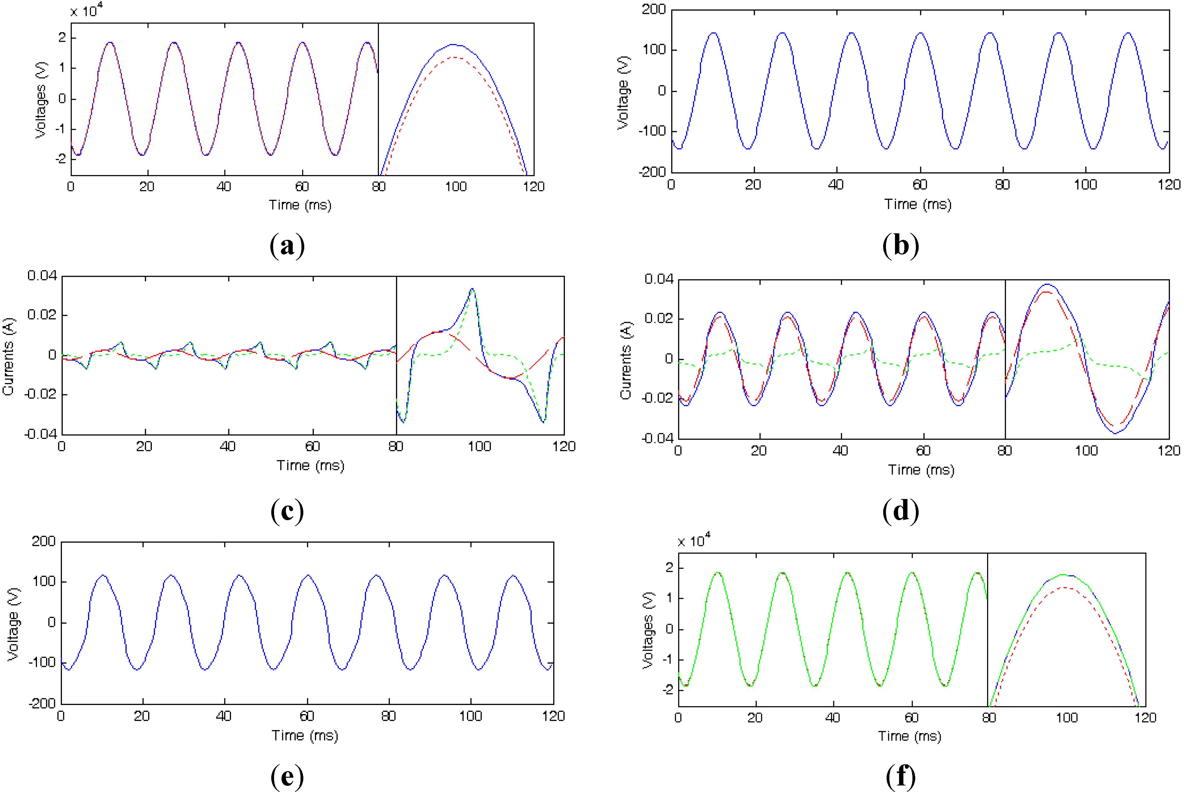
3.1. Case 1: 120% of the Rated Voltage

Figure 7 shows the results for Case 1. In Figure 7a, the solid and dotted lines indicate v₁ and av₂, respectively. The difference between v₁ and av₂ is v_p + av_s, which causes the error of the VT. Figure 7b shows the secondary winding voltage av_s, which is calculated by using Equation (2). In Figure 7c, the dashed, dotted, and solid lines indicate i_c calculated by using Equation (9), i_m calculated by using the λ-i_m curve, and i₀ calculated by using Equation (6), respectively. In Figure 7d, the solid, dotted, and dashed lines indicate i₁, i₀, and i₂/a, respectively. i₂/a is nearly sinusoidal, while i₁ is non-sinusoidal due to i₀. Figure 7e shows v_p, which is also the non-sinusoidal wave and is similar in shape to i₁. This is because R₁ is significantly larger than L₁. In Figure 7f, the solid, dotted, and dashed lines represent v₁, av₂, and the compensated secondary voltage (v_comp), which is obtained by using Equation (1), respectively. v_comp is nearly the same as v₁ as shown in Figure 7f. Portions of the figures are expanded to see the performance of the proposed scheme. The results of the ratio and phase errors for Case 1 are shown in Table 2. The ratio and phase errors of the measured voltage are −1.422% and 7.732 min, respectively, which are larger than those obtained using the 1.0C class in Table 1. However, the ratio and phase errors of the compensated voltage are 0.0002% and −0.1 min, which are much less than 0.1C class. The results signify that the proposed compensation scheme can eliminate the errors of the VT caused by the primary and secondary winding voltages.

Figure 7. Results for Case 1: (a) v₁ (solid) and av₂ (dotted); (b) av_s; (c) i₀ (solid), i_m (dotted), and i_c (dashed); (d) i₁ (solid), i₀ (dotted), and i₂/a (dashed); (e) v_p; and (f) v₁ (solid), av₂ (dotted), and v_comp (dashed).

Figure 7. Results for Case 1: (a) v₁ (solid) and av₂ (dotted); (b) av_s; (c) i₀ (solid), i_m (dotted), and i_c (dashed); (d) i₁ (solid), i₀ (dotted), and i₂/a (dashed); (e) v_p; and (f) v₁ (solid), av₂ (dotted), and v_comp (dashed).

Table 2. Errors for 120% of the rated voltage.

Error	Measured Voltage	Compensated Voltage
Ratio error (%)	–1.422	0.0002
Phase error (min)	7.732	–0.1

Table 2. Errors for 120% of the rated voltage.

Error	Measured Voltage	Compensated Voltage
Ratio error (%)	–1.422	0.0002
Phase error (min)	7.732	–0.1

3.2. Case 2: 100% of the Rated Voltage

Figure 8 shows the results for Case 2. Figure 8a shows that av₂ differs from v₁. As shown in Table 3, the ratio and phase errors of the measured voltage are −1.414% and 2.93 min, respectively, which are larger than for the 1.0C class in Table 1 and smaller than in Case 1. Figure 8c shows that i_m in Case 2 is significantly smaller than in Case 1, and thus the non-sinusoidal component contained in i₁ is also small. Figure 8e indicates that v₁ and v_comp are nearly identical. The ratio and phase errors of the compensated voltage are 0.001% and −0.03 min, which are much less than those of the 0.1C class.

Figure 8. Results for Case 2: (a) v₁ (solid) and av₂ (dotted); (b) av_s; (c) i₀ (solid), i_m (dotted), and i_c (dashed); (d) i₁ (solid), i₀ (dotted), and i₂/a (dashed); (e) v_p; and (f) v₁ (solid), av₂ (dotted), and v_comp (dashed).

Figure 8. Results for Case 2: (a) v₁ (solid) and av₂ (dotted); (b) av_s; (c) i₀ (solid), i_m (dotted), and i_c (dashed); (d) i₁ (solid), i₀ (dotted), and i₂/a (dashed); (e) v_p; and (f) v₁ (solid), av₂ (dotted), and v_comp (dashed).

Table 3. Errors for 100% of the rated voltage.

Error	Measured Voltage	Compensated Voltage
Ratio error (%)	–1.414	0.001
Phase error (min)	2.93	–0.03

Table 3. Errors for 100% of the rated voltage.

Error	Measured Voltage	Compensated Voltage
Ratio error (%)	–1.414	0.001
Phase error (min)	2.93	–0.03

3.3. Case 3: 80% of the Rated Voltage

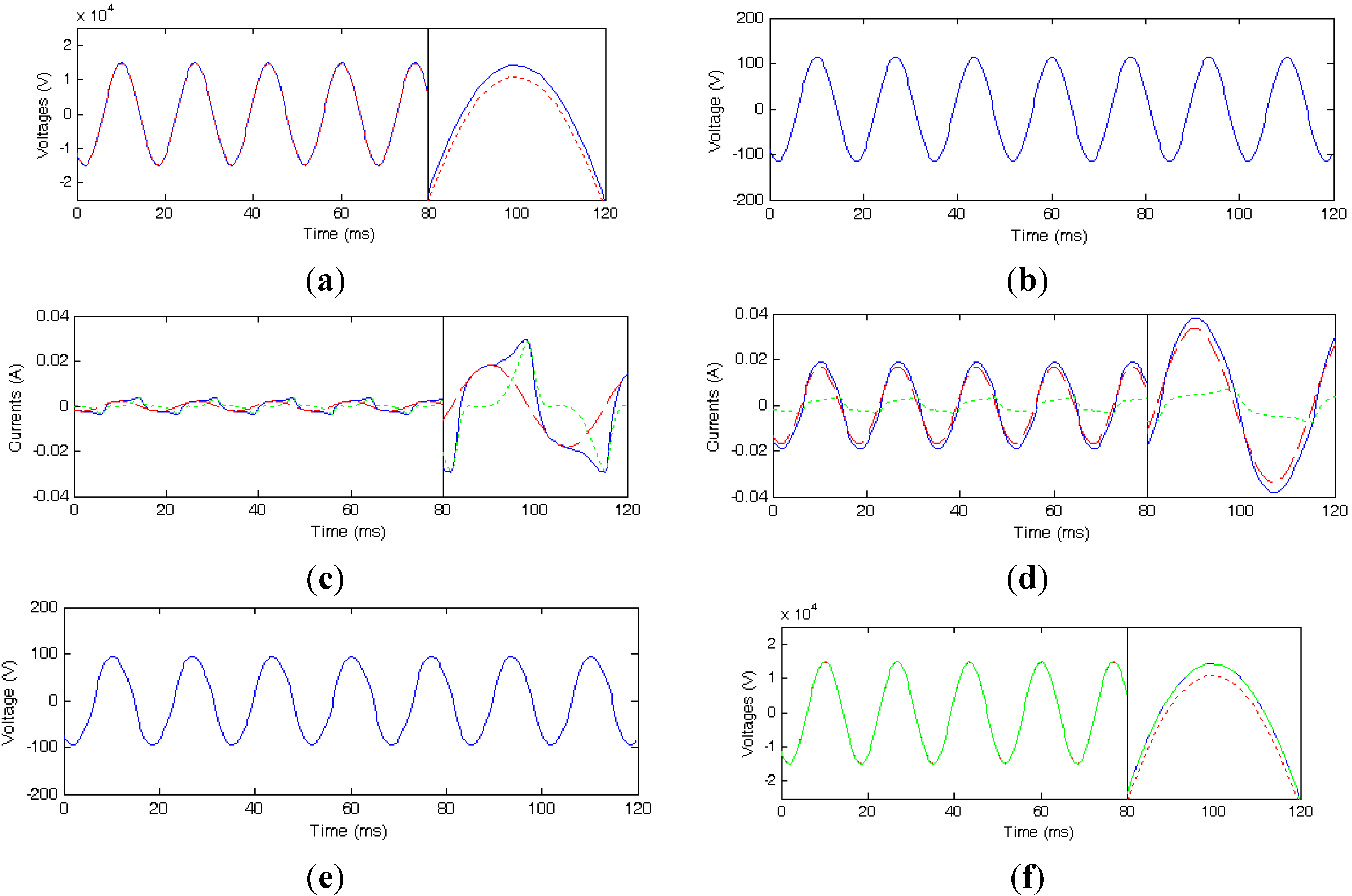
Figure 9 shows the results for Case 3. As shown in Table 4, the ratio and phase errors of the measured voltage are −1.424% and 2.167 min, respectively, which are larger than those of 1.0C class, smaller than in Case 1, and similar to those in Case 2. As shown in Figure 9b–c, the non-sinusoidal components in i₀ and i₁ are smaller than in Case 1, but are similar to those in Case 2. Figure 9d shows that v₁ is nearly the same as v_comp. The ratio and phase errors of the compensated voltage are 0.0001% and −0.002 min, which are much less than those of 0.1C class.

Figure 9. Results for Case 3: (a) v₁ (solid) and av₂ (dotted); (b) av_s; (c) i₀ (solid), i_m (dotted), and i_c (dashed); (d) i₁ (solid), i₀ (dotted), and i₂/a (dashed); (e) v_p; and (f) v₁ (solid), av₂ (dotted), and v_comp (dashed).

Figure 9. Results for Case 3: (a) v₁ (solid) and av₂ (dotted); (b) av_s; (c) i₀ (solid), i_m (dotted), and i_c (dashed); (d) i₁ (solid), i₀ (dotted), and i₂/a (dashed); (e) v_p; and (f) v₁ (solid), av₂ (dotted), and v_comp (dashed).

Table 4. Errors for 80% of the rated voltage.

Error	Measured Voltage	Compensated Voltage
Ratio error (%)	–1.424	0.0001
Phase error (min)	2.167	–0.002

Table 4. Errors for 80% of the rated voltage.

Error	Measured Voltage	Compensated Voltage
Ratio error (%)	–1.424	0.0001
Phase error (min)	2.167	–0.002

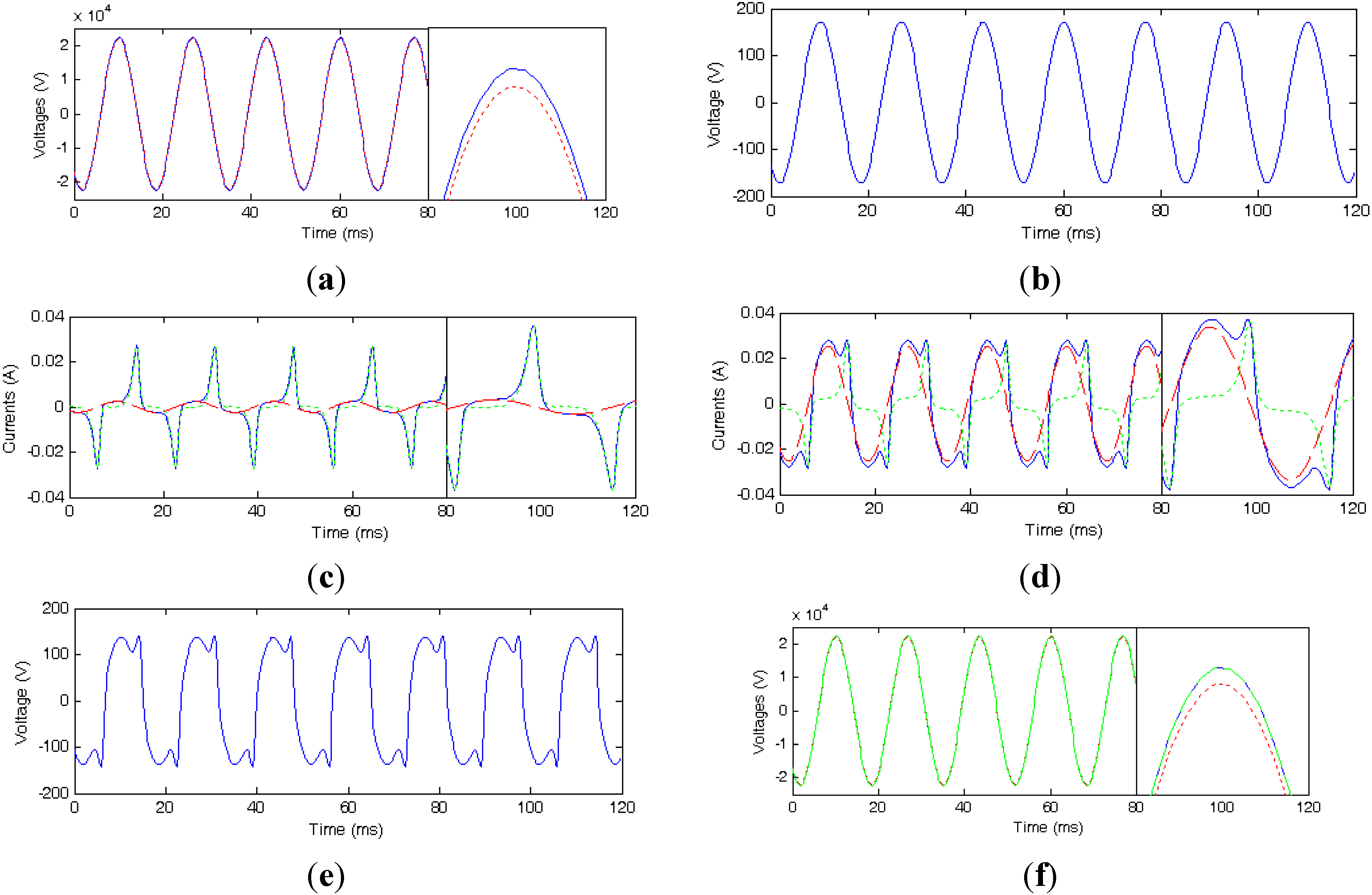
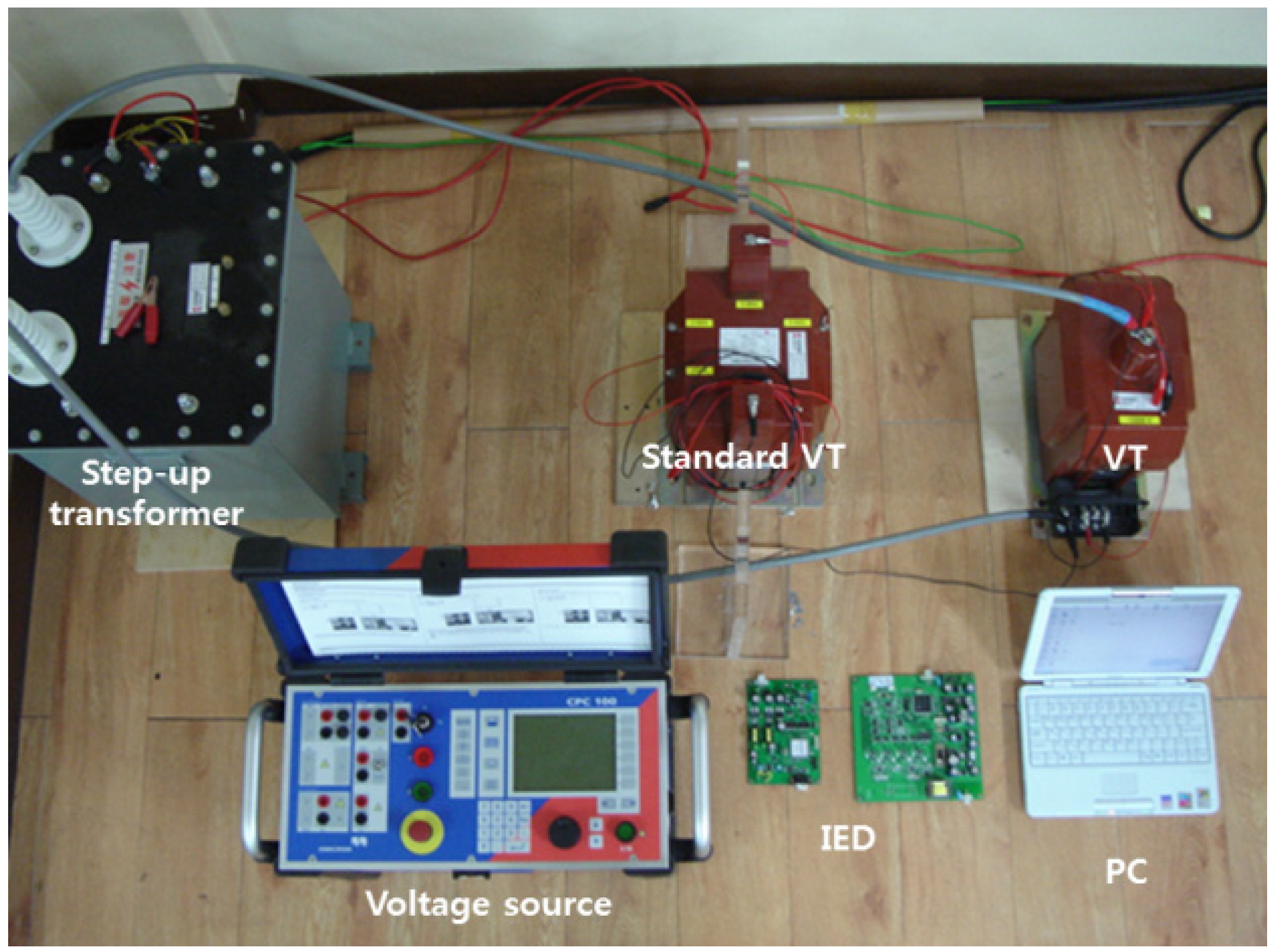
4. Experimental Test Results

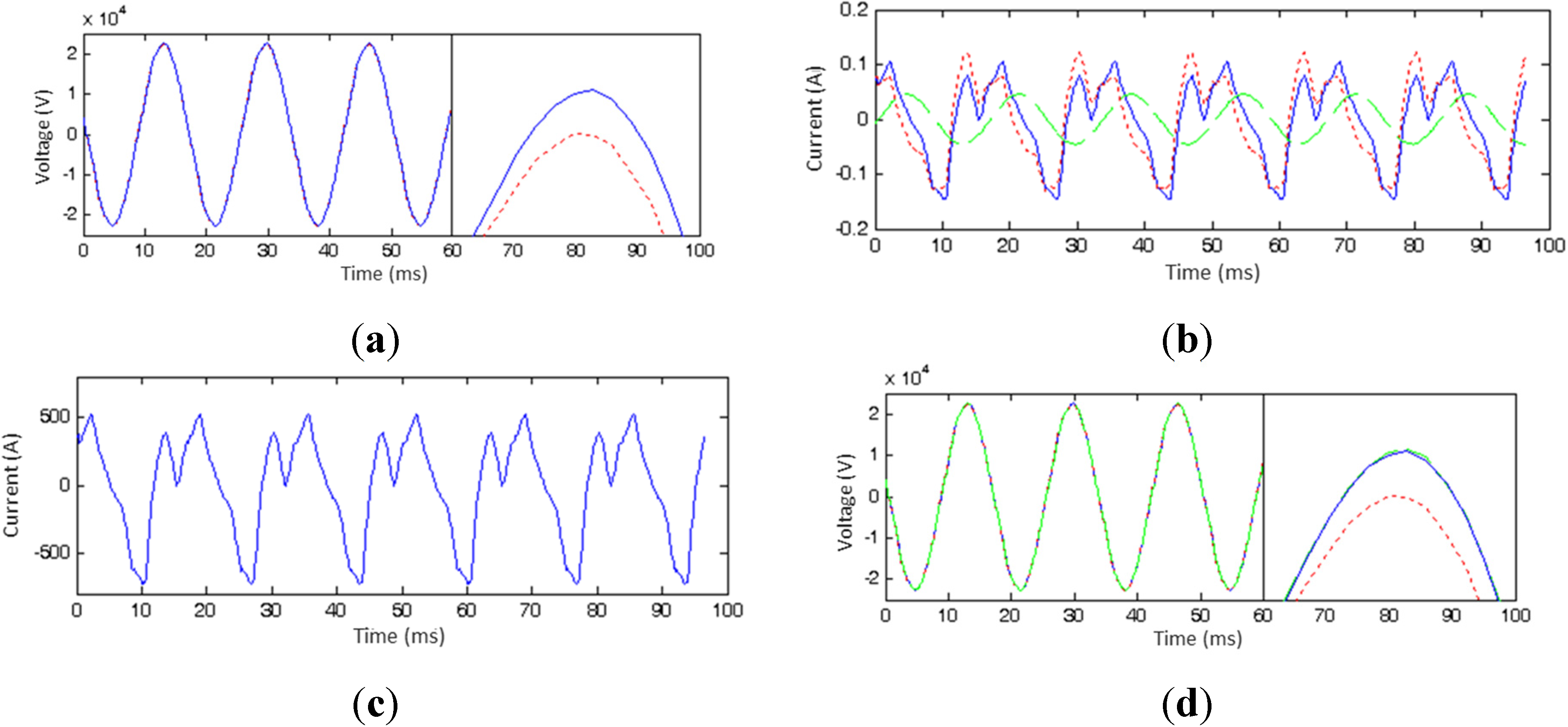
To validate that the proposed compensation scheme obtains high accuracy and satisfactory real-time results under conditions with plentiful noise, a series of experiments were conducted on a real measurement VT. Figure 10 shows the configuration of the test system, which consists of a voltage source, a step-up transformer, a standard VT with a high accuracy of 0.1C, a VT for test, an intelligent electronic device (IED), and a PC. To implement the proposed compensation scheme, the IED based on a TMS320C2812 DSP (Texas Instruments, Dallas, TX, USA) and a VT (13,200/110 V and R_b = 60.5 Ω) are used. The voltage, which is provided by the voltage source and step-up transformer, is applied to the load and provides the voltage across the tested VT. The voltage across the burden of the VT is measured and used to calculate the exciting current, primary winding voltage, and secondary winding voltage. The sampling rate of 64 samples/cycle was used, and all of the signals are passed through the first order RC filters with a cutoff frequency of 1920 Hz.

Figure 10. Configuration of the experimental test system.

Figure 10. Configuration of the experimental test system.

Figure 11, Figure 12 and Figure 13 show the experimental test results for 120%, 100%, and 80% of the rated voltage. The ratio and phase errors of the measured and compensated voltages are shown in Table 5. The results of experimental test have the errors due to the noise and A/D conversion. Thus, in terms of the accuracy of the compensated voltages, the experimental test is larger than the simulation results.

Figure 11. Results for 120% of the rated voltage: (a) v₁ (solid) and av₂ (dotted); (b) i₀ (solid), i_m (dotted), and i_c (dashed); (c) v_p; and (d) v₁ (solid), av₂ (dotted), and v_comp (dashed).

Figure 11. Results for 120% of the rated voltage: (a) v₁ (solid) and av₂ (dotted); (b) i₀ (solid), i_m (dotted), and i_c (dashed); (c) v_p; and (d) v₁ (solid), av₂ (dotted), and v_comp (dashed).

Figure 12. Results for 100% of the rated voltage: (a) v₁ (solid) and av₂ (dotted); and (b) v₁ (solid), av₂ (dotted), and v_comp (dashed).

Figure 12. Results for 100% of the rated voltage: (a) v₁ (solid) and av₂ (dotted); and (b) v₁ (solid), av₂ (dotted), and v_comp (dashed).

Figure 13. Results for 80% of the rated voltage: (a) v₁ (solid) and av₂ (dotted); and (b) v₁ (solid), av₂ (dotted), and v_comp (dashed).

Figure 13. Results for 80% of the rated voltage: (a) v₁ (solid) and av₂ (dotted); and (b) v₁ (solid), av₂ (dotted), and v_comp (dashed).

Table 5. Results for the experimental test.

Case	Error	Measured Voltage	Compensated Voltage
120% of the rated voltage	Ratio error (%)	0.1997	0.01884
	Phase error (min)	69.82	1.009
100% of the rated voltage	Ratio error (%)	0.1301	0.08048
	Phase error (min)	65.03	0.2075
80% of the rated voltage	Ratio error (%)	‒1.758	0.01571
	Phase error (min)	64.38	0.3567

Table 5. Results for the experimental test.

Case	Error	Measured Voltage	Compensated Voltage
120% of the rated voltage	Ratio error (%)	0.1997	0.01884
	Phase error (min)	69.82	1.009
100% of the rated voltage	Ratio error (%)	0.1301	0.08048
	Phase error (min)	65.03	0.2075
80% of the rated voltage	Ratio error (%)	‒1.758	0.01571
	Phase error (min)	64.38	0.3567

However, the errors are less than those of 0.1C class. The results indicate that the scheme can significantly improve the accuracy of the VT from 1.5C class (uncompensated) to 0.1C class (compensated).

5. Conclusions

In this paper, a compensation scheme for the iron-cored measurement VT was proposed considering the hysteresis characteristics of the core in the time domain. The secondary current is obtained directly from the secondary voltage and is used to obtain the voltage across the secondary winding. The exciting current is decomposed into the core-loss and magnetizing currents in this paper. To obtain the magnetizing current, the flux-magnetizing current curve is used instead of the hysteresis loop. The core-loss current is obtained by dividing the primary induced voltage by the core-loss resistance. Finally, the estimated voltages across the primary and secondary windings are added to the measured secondary voltage for compensation.

The performance of the proposed compensation scheme was validated in a typical Korean distribution system for 120%, 100%, and 80% of the rated voltage. The simulation results demonstrated that the scheme can compensate the measured secondary voltage and thus significantly improve the accuracy of a VT from 1.0C class to 0.1C class. In the experimental test, the accuracy of the measurement VT is improved from 1.5C class to 0.1C class through the compensator. The experimental test results also demonstrate that the compensator can improve the accuracy of the measurement VT from 1.5C class to 0.1C class. The proposed scheme can not only improve the accuracy of a measurement VT, but also significantly reduce the required core cross section of a VT.

References

1. International Electrotechnical Commission (IEC). International standard IEC 60044–7: “Instrument transformer—Part 7: Electronic Voltage Transformers”. IEC: Geneva, Switzerland, 1999. [Google Scholar]
2. IEEE Power Engineering Society. IEEE Std.. C57.13-2008: IEEE standard requirements for instrument transformers. Available online: http://ieeexplore.ieee.org/xpl/articleDetails.jsp?arnumber=4581634 (accessed on 20 April 2015).
3. IEEE Power Engineering Society. IEEE Std.. C57.13.6-2005: IEEE standard for high-accuracy instrument transformers. Available online: http://ieeexplore.ieee.org/servlet/opac?punumber=10453 (accessed on 20 April 2015).
4. Slomovitz, D. Electronic compensation of voltage transformer. IEEE Trans. Instrum. Meas. 1988, 37, 652–654. [Google Scholar] [CrossRef]
5. Slomovitz, D. Electronic based high-voltage measuring transformer. IEEE Trans. Power Deliv. 2002, 17, 359–361. [Google Scholar] [CrossRef]
6. Kang, Y.C.; Zheng, T.Y.; Kim, Y.H.; Lee, B.E.; So, S.H.; Crossley, P.A. Development of compensation algorithm for a measurement current transformer. IET Gener. Trans. Distr. 2011, 5, 531–539. [Google Scholar]
7. Terashima, K.; Wada, K.; Shimizu, T.; Nakazawa, T.; Ishii, K.; Hayashi, Y. Evaluation of the iron loss of an inductor based on dynamic minor characteristics. In Proceedings of the Power Electronics and Applications, 2007 European Conference, Dresden, Germany, 2–5 September 2007; pp. 1–8.
8. Kang, Y.C.; Park, J.K.; Kang, S.H.; Johns, A.T.; Aggarwal, R.K. An algorithm for compensating secondary currents of current transformers. IEEE Trans. Power Deliv. 1997, 12, 116–124. [Google Scholar] [CrossRef]
9. Kezunovic, M.; Kojovic, L.; Abur, A.; Fromen, C.W.; Sevcik, D.R.; Phillips, F. Experimental evaluation of EMTP-based current transformer models for protective relay transient study. IEEE Trans. Power Deliv. 1994, 9, 405–413. [Google Scholar] [CrossRef]