
Modelling Wind for Wind Farm Layout Optimization Using Joint Distribution of Wind Speed and Wind Direction


Abstract
:1. Introduction
2. Background
2.1. Wind Farm Layout Optimization
2.2. Wind Modelling


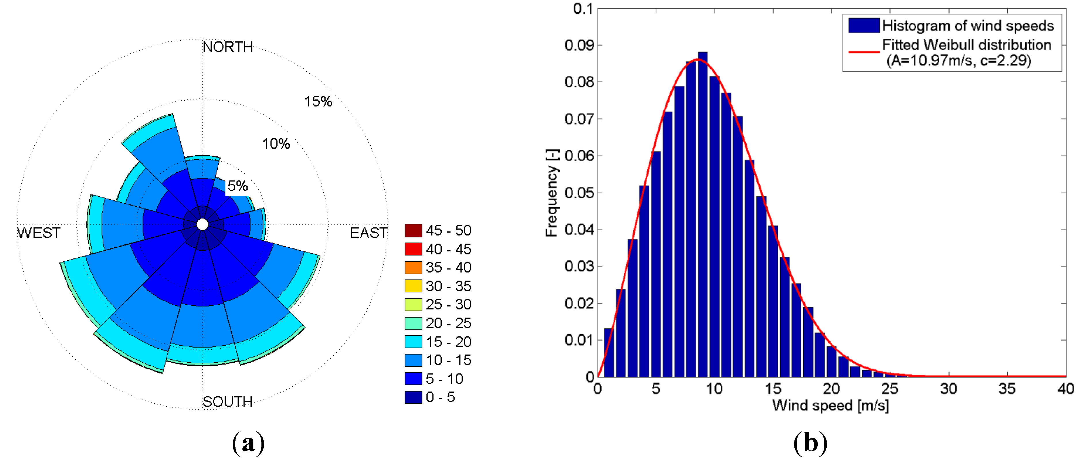
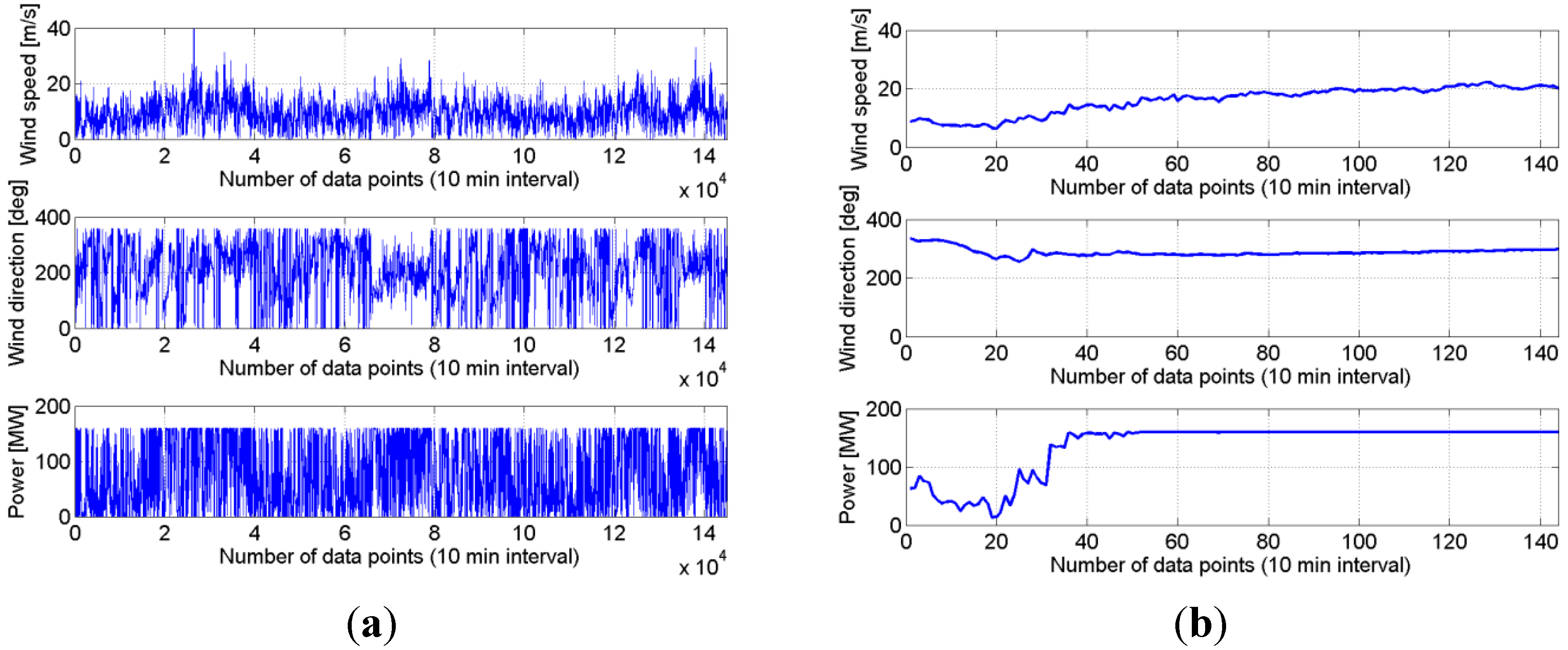
3. Data Source


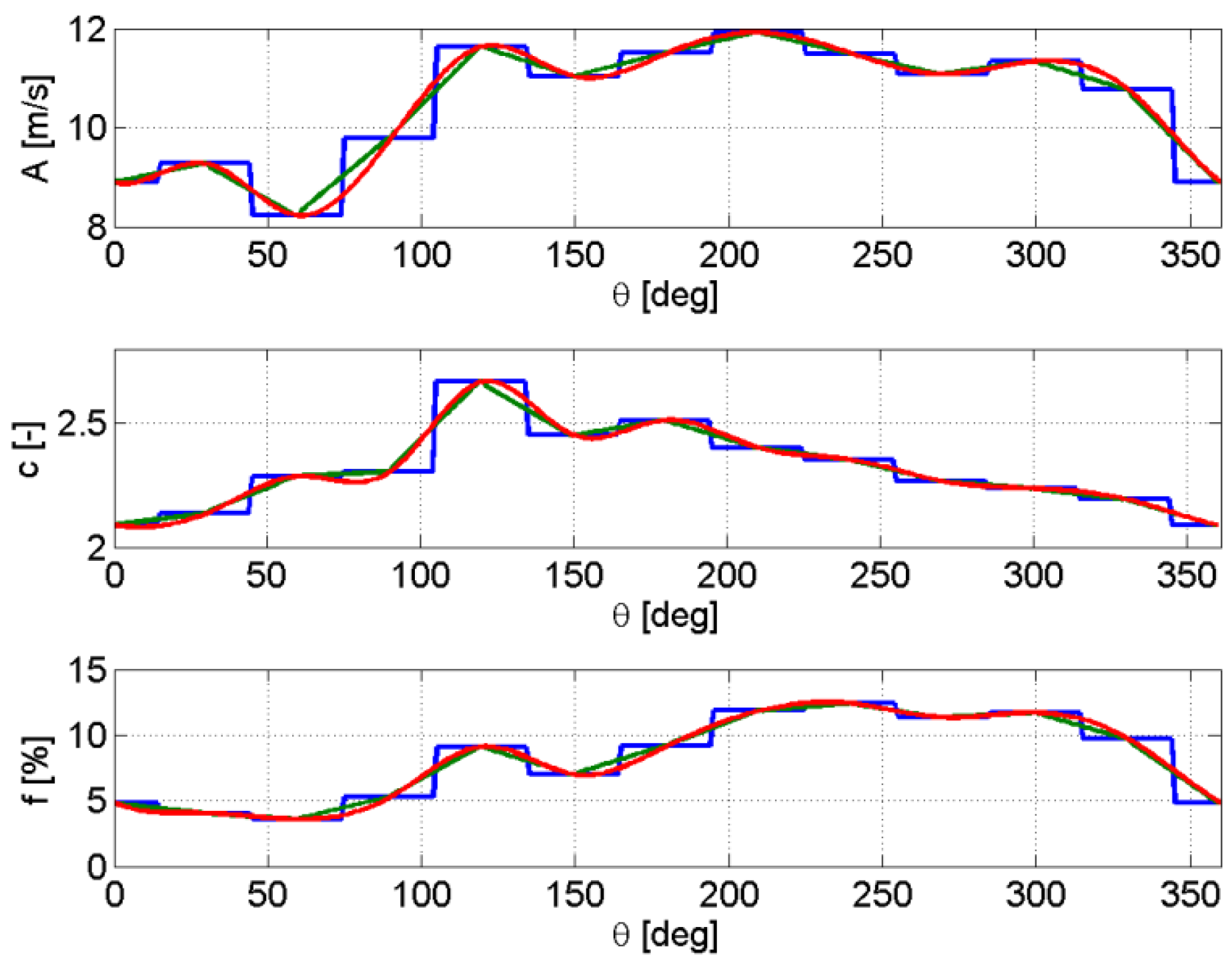
| θ Direction | 0° N | 30° NNE | 60° ENE | 90° E | 120° ESE | 150° SSE | 180° S | 210° SSW | 240° WSW | 270° W | 300° WNW | 330° NNW |
|---|---|---|---|---|---|---|---|---|---|---|---|---|
| 8.89 | 9.27 | 8.23 | 9.78 | 11.64 | 11.03 | 11.50 | 11.92 | 11.49 | 11.08 | 11.34 | 10.76 | |
| 2.09 | 2.13 | 2.29 | 2.30 | 2.67 | 2.45 | 2.51 | 2.40 | 2.35 | 2.27 | 2.24 | 2.19 | |
| 4.82 | 4.06 | 3.59 | 5.27 | 9.12 | 6.97 | 9.17 | 11.84 | 12.41 | 11.34 | 11.70 | 9.69 |
4. Construction of Joint Distributions
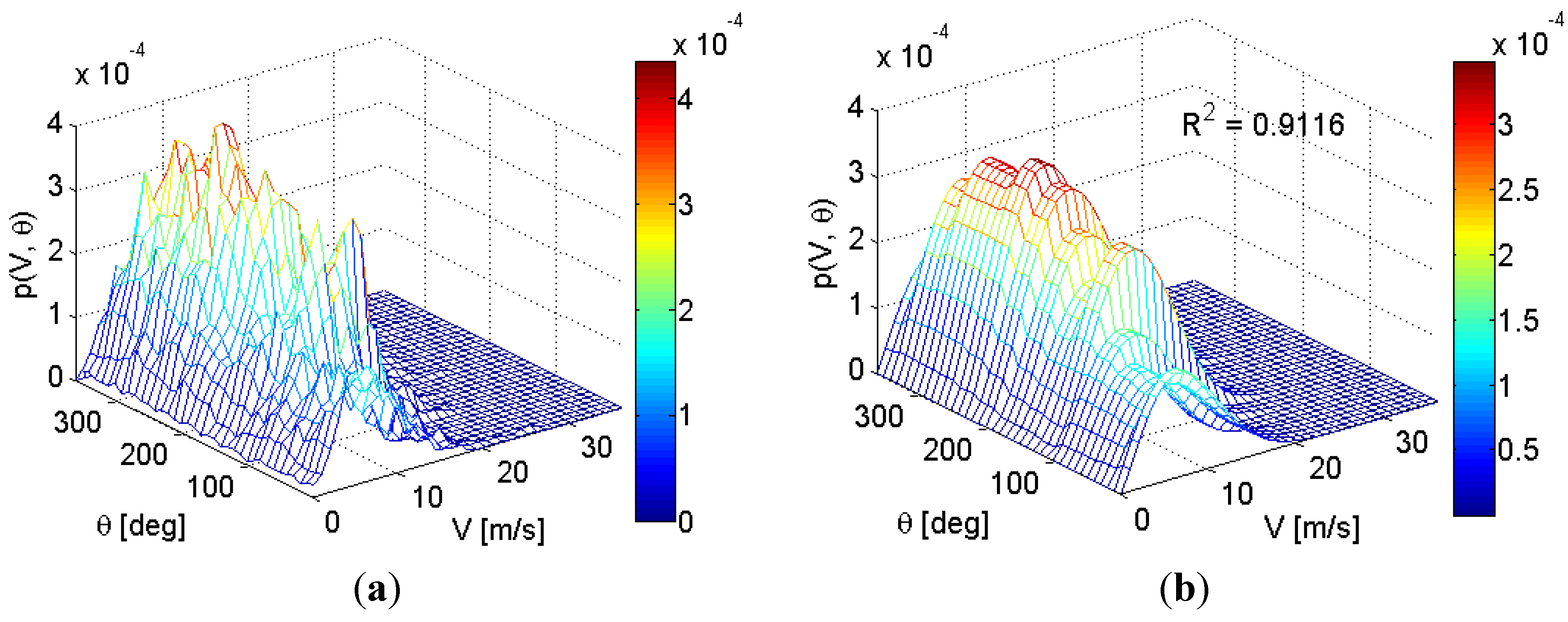
4.1. Piecewise Bivariate PDF

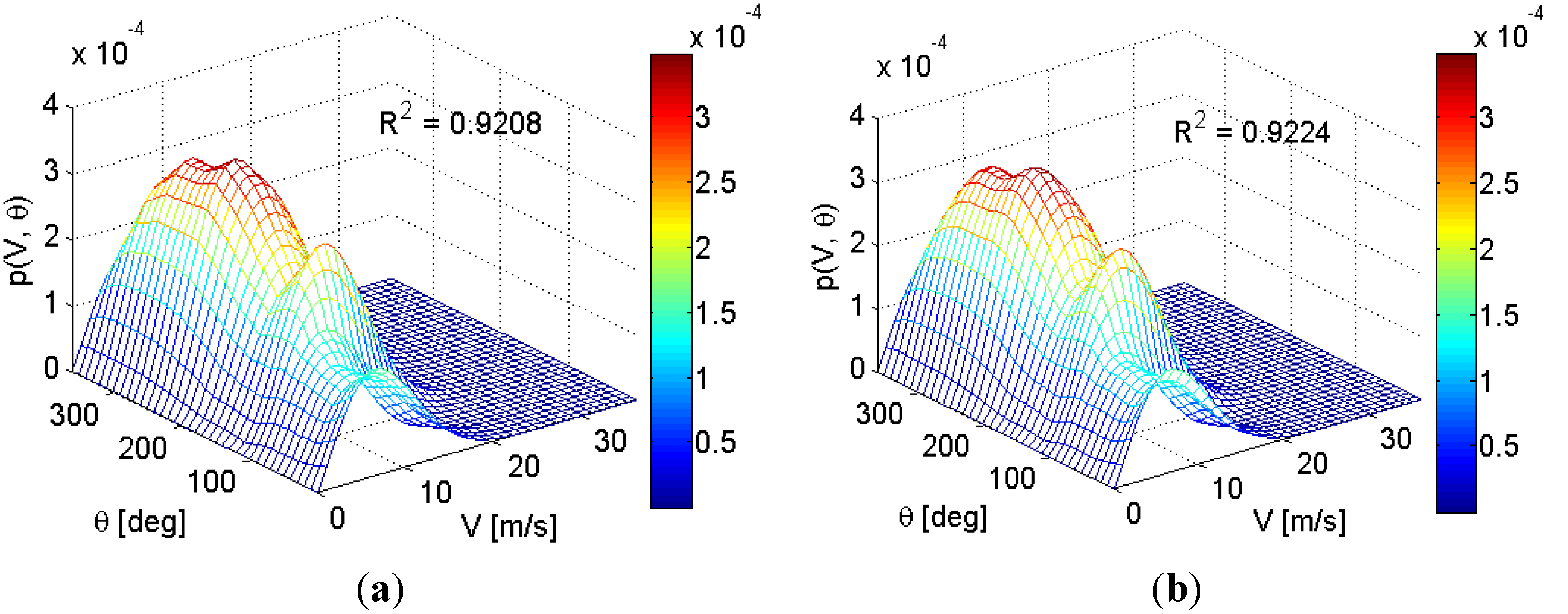
4.2. Continuous Joint Distributions

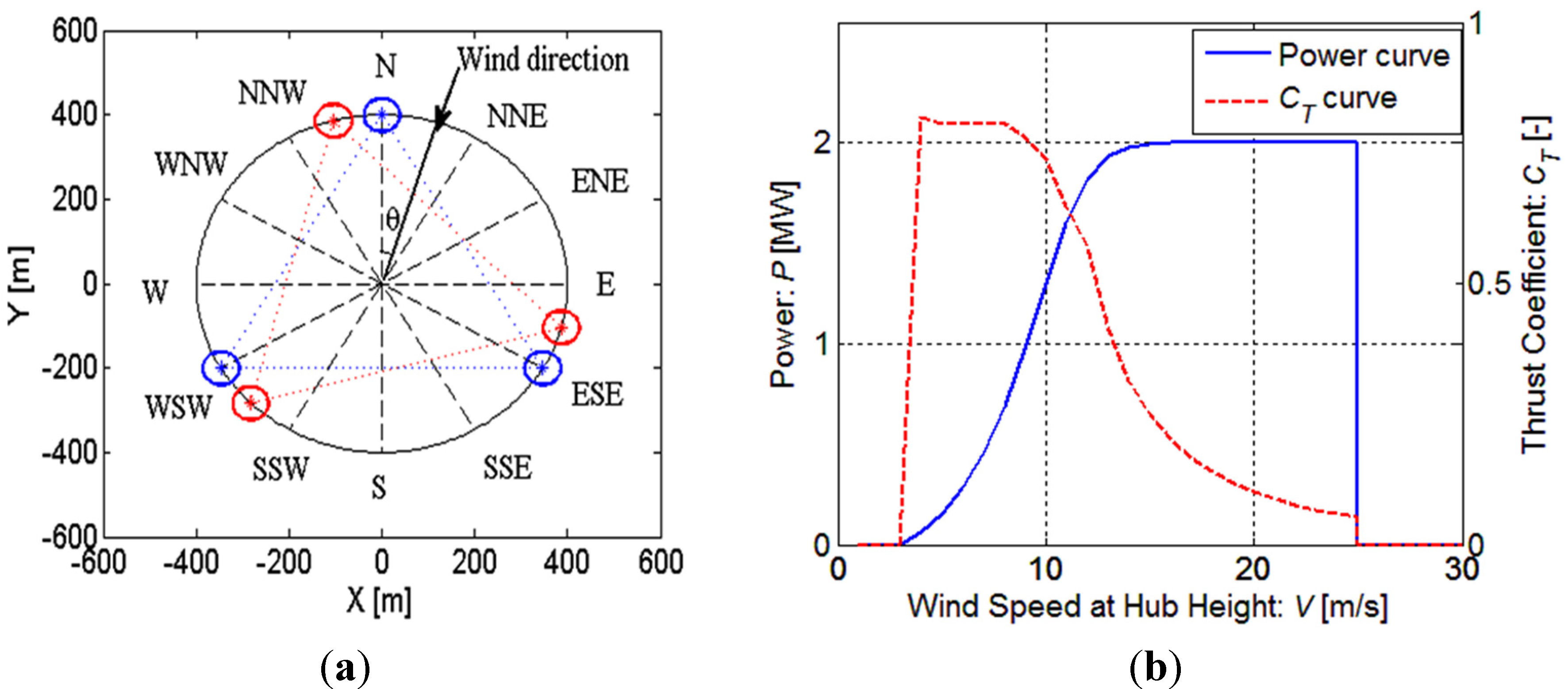
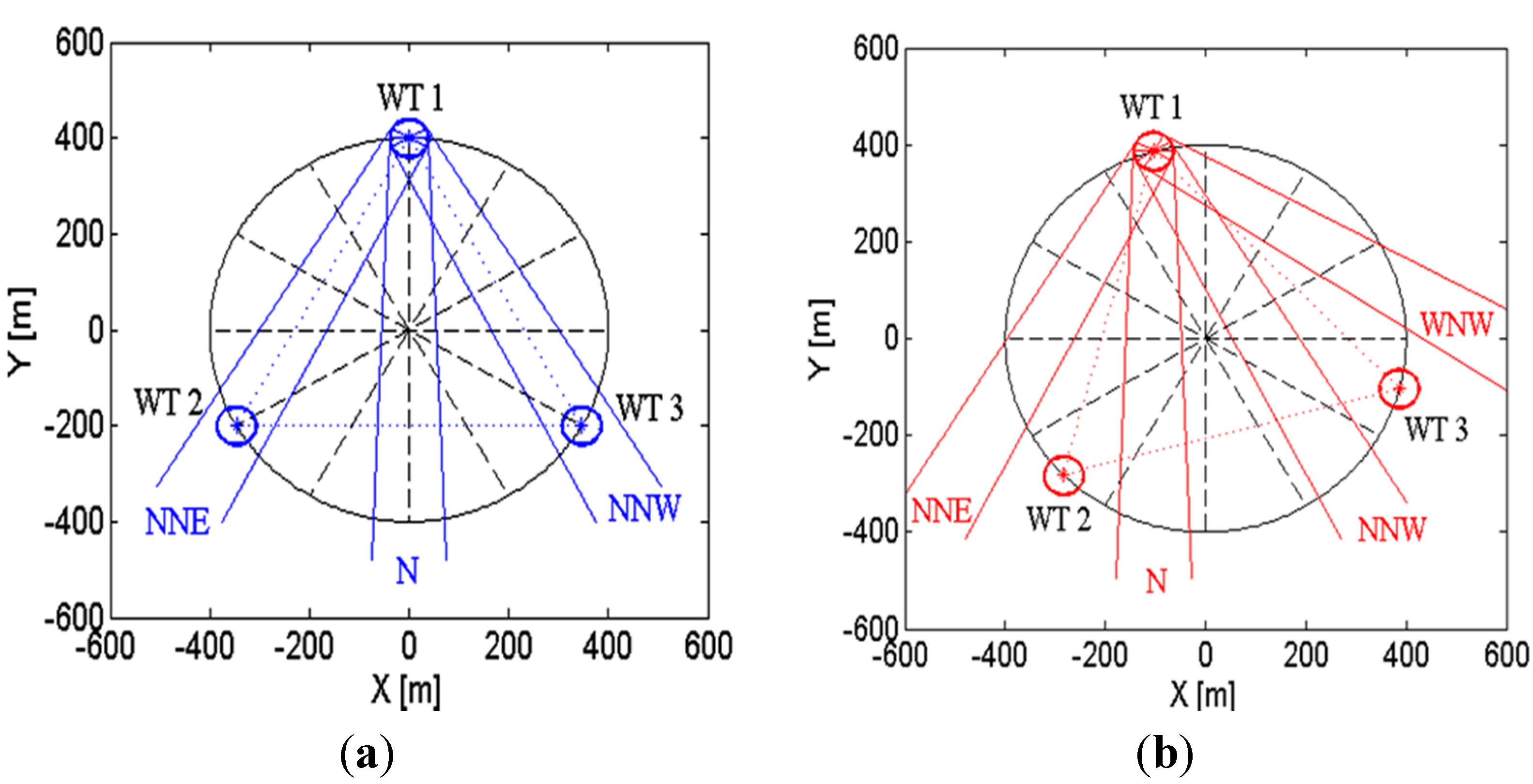
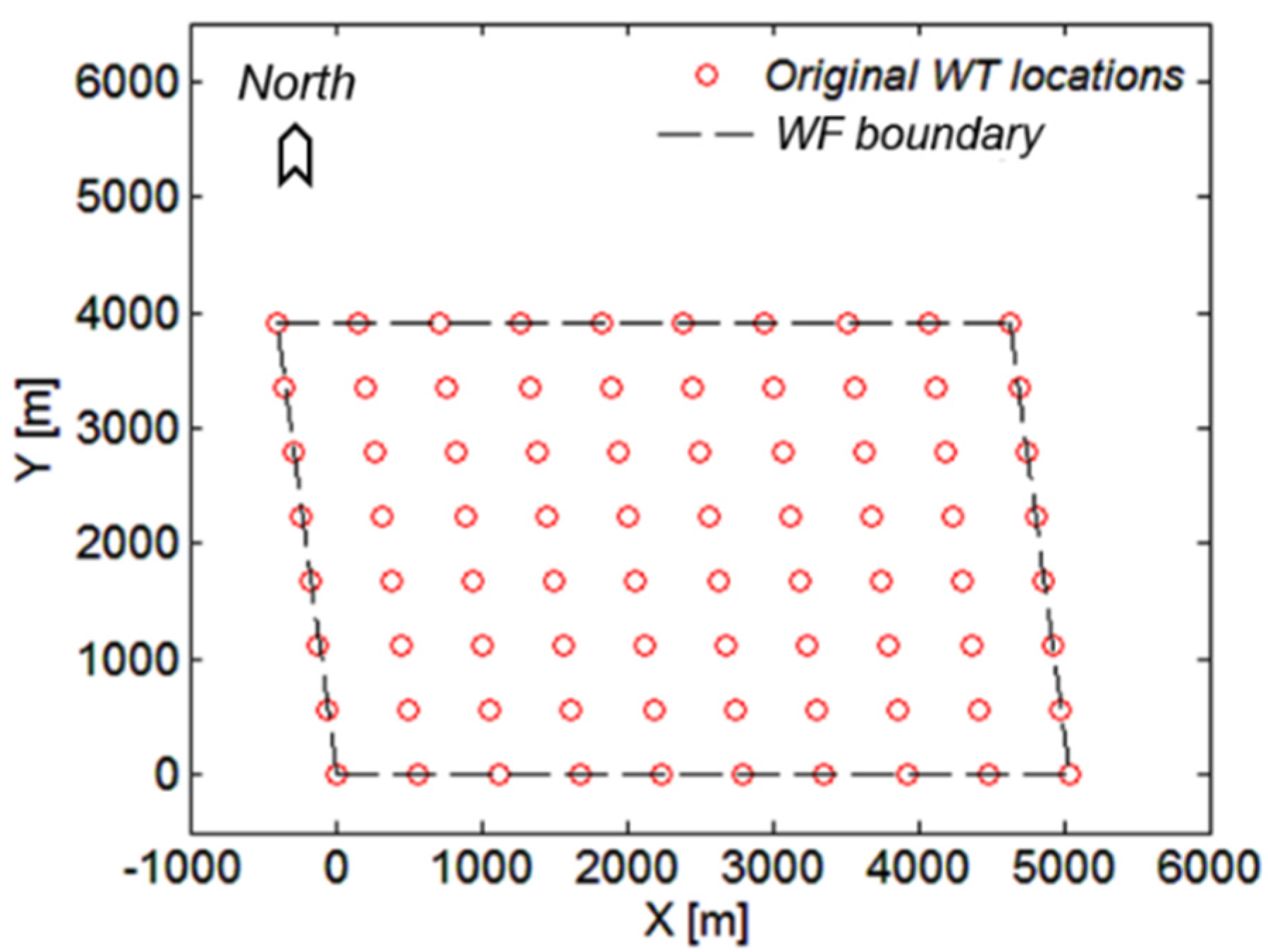
5. Application in Wind Farm Layout Optimization

5.1. Assessment of Bin Sizes for Power Calculation
| Δv [m/s] | Δθ = 30° | Δθ = 10° | Δθ = 5° | Δθ = 3° | Δθ = 1° |
|---|---|---|---|---|---|
| Ptot (using piecewise joint distribution) | |||||
| 2 | 77.13 MW | 78.80 MW | 78.93 MW | 79.02 MW | 78.86 MW |
| 1 | 76.86 MW | 78.57 MW | 78.69 MW | 78.78 MW | 78.63 MW |
| 0.5 | 76.85 MW | 78.53 MW | 78.65 MW | 78.74 MW | 78.59 MW |
| 0.1 | 76.85 MW | 78.54 MW | 78.65 MW | 78.75 MW | 78.59 MW |
| Ptot (using linear joint distribution) | |||||
| 2 | 77.13 MW | 78.44 MW | 78.49 MW | 78.58 MW | 78.42 MW |
| 1 | 76.86 MW | 78.22 MW | 78.26 MW | 78.35 MW | 78.20 MW |
| 0.5 | 76.85 MW | 78.19 MW | 78.21 MW | 78.30 MW | 78.15 MW |
| 0.1 | 76.85 MW | 78.19 MW | 78.22 MW | 78.31 MW | 78.16 MW |
| Ptot (using spline joint distribution) | |||||
| 2 | 77.13 MW | 78.84 MW | 78.94 MW | 79.04 MW | 78.89 MW |
| 1 | 76.86 MW | 78.61 MW | 78.70 MW | 78.80 MW | 78.66 MW |
| 0.5 | 76.85 MW | 78.58 MW | 78.66 MW | 78.75 MW | 78.62 MW |
| 0.1 | 76.85 MW | 78.58 MW | 78.66 MW | 78.77 MW | 78.62 MW |
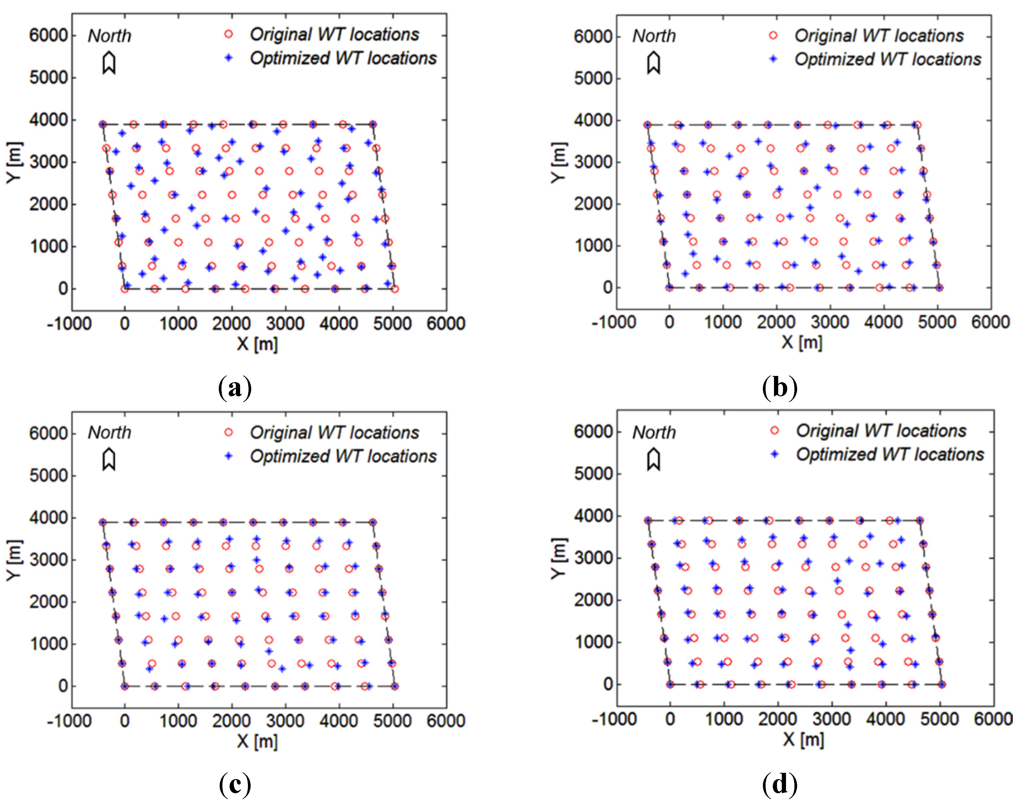
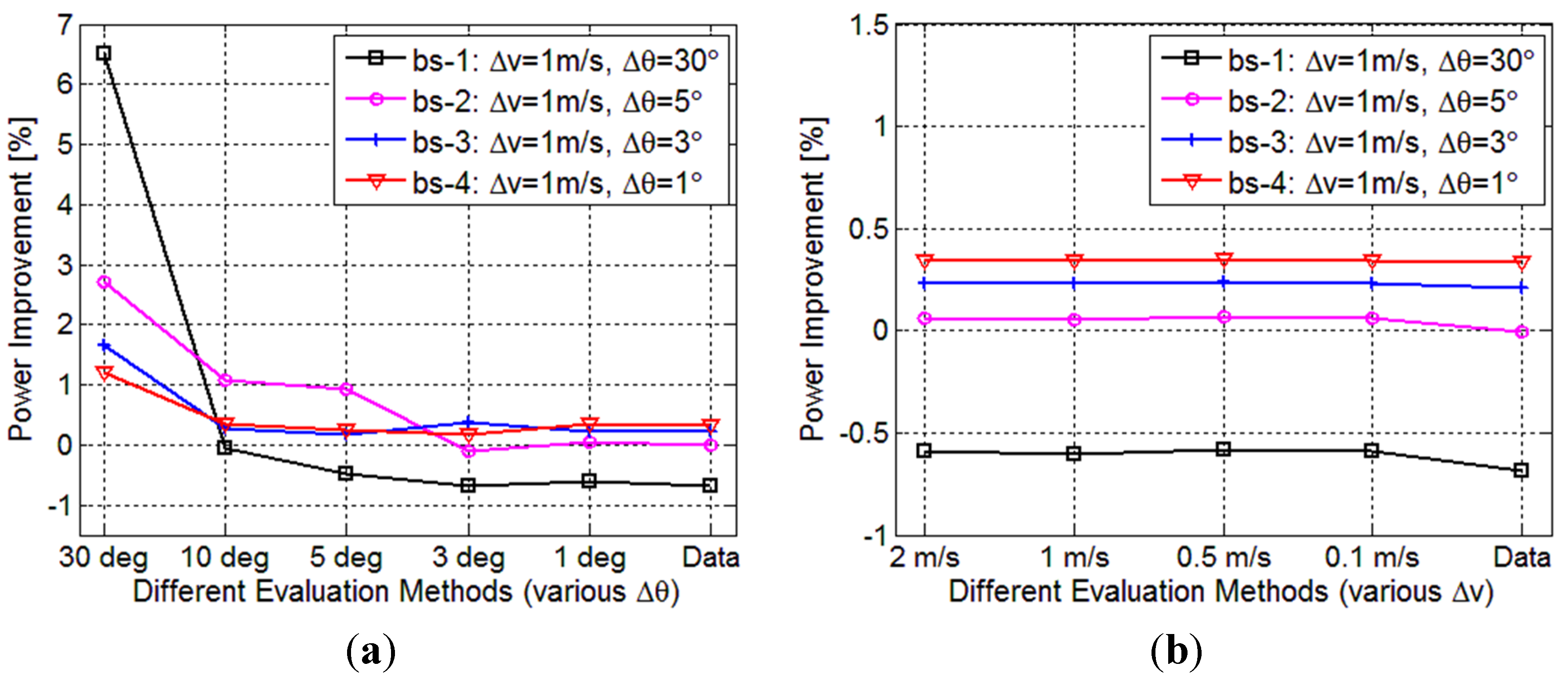
5.2. Choice of Bin Size Δθ for Layout Optimization
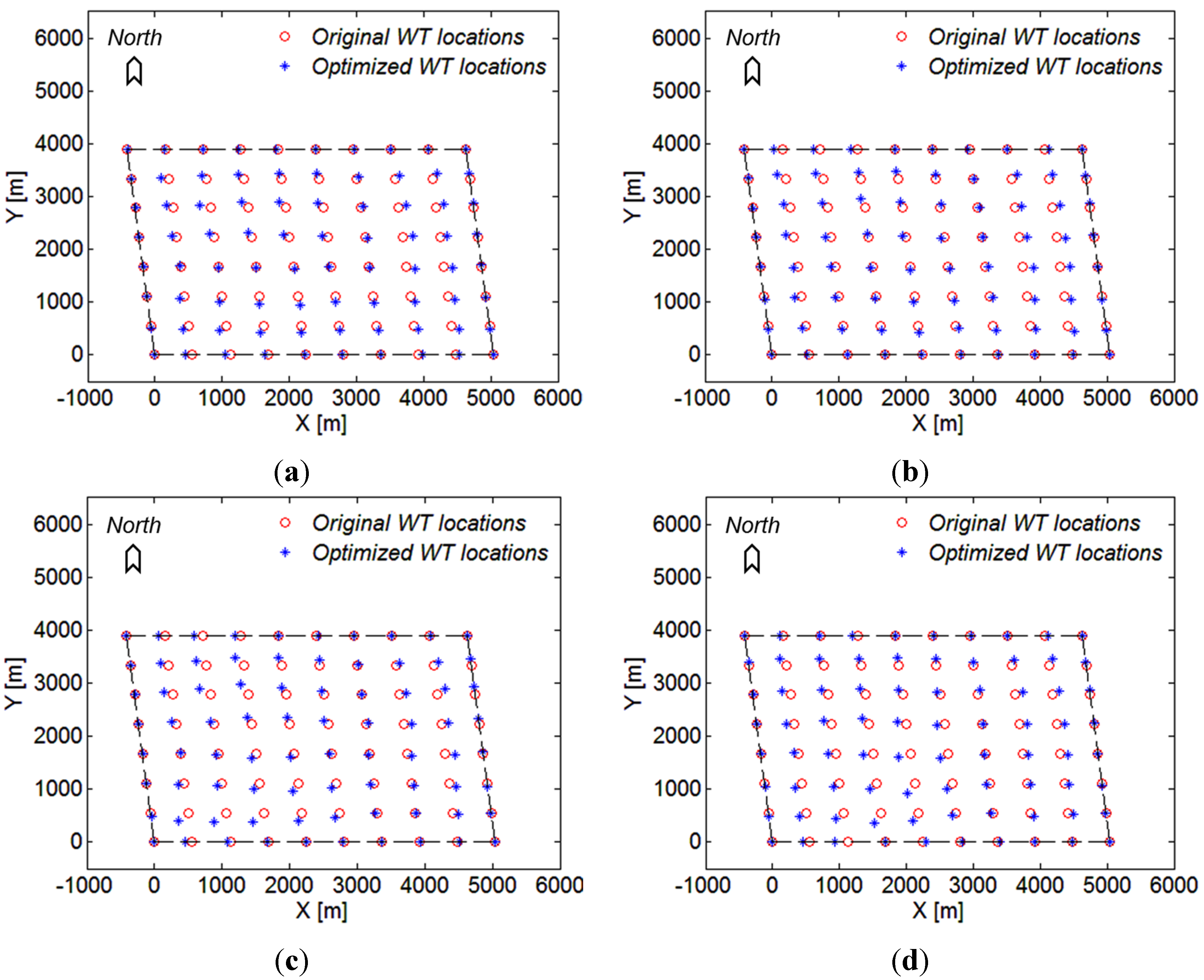
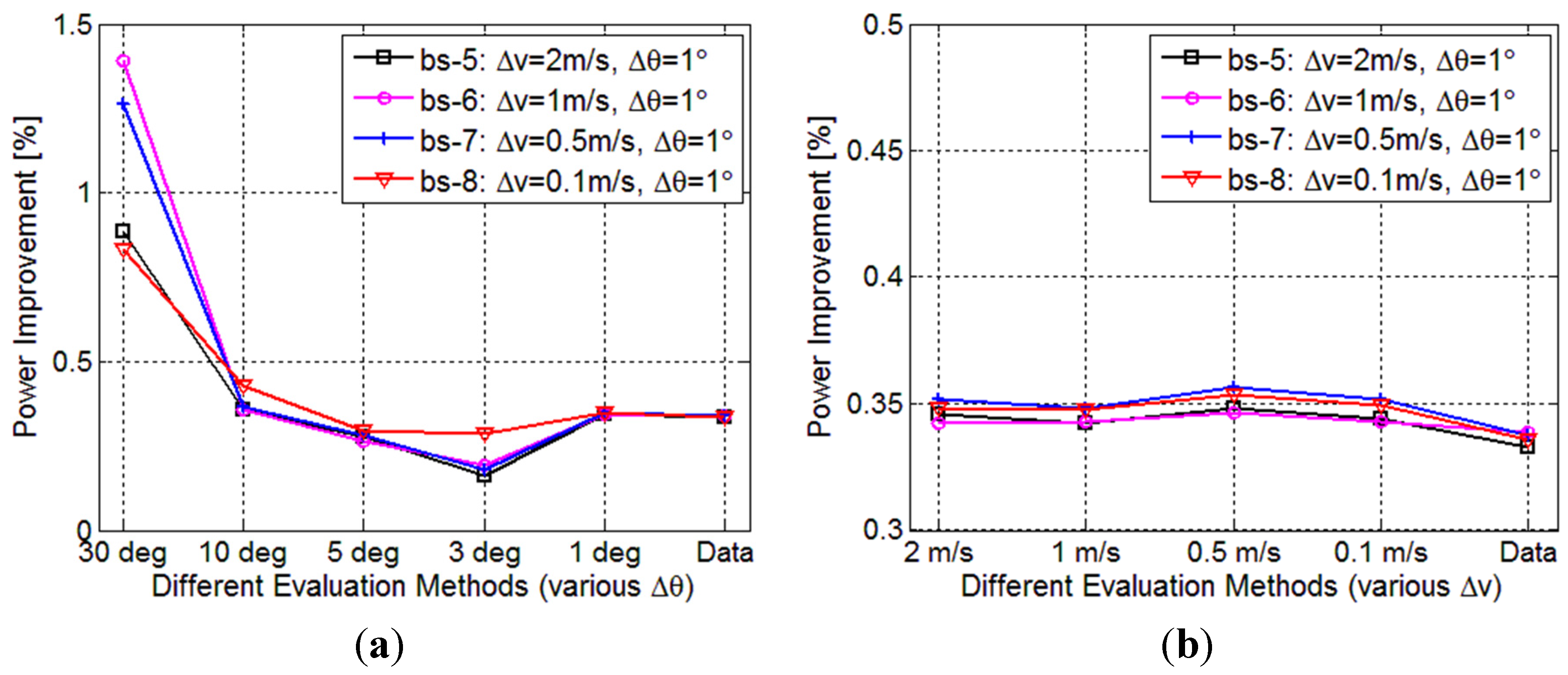
5.3. Choice of Bin Size Δv for Layout Optimization
- The proposed continuous joint distributions of wind speed and wind direction can be applied in both wind farm power calculation and layout optimization;
- The common practice of using Δv =1 m/s and Δθ = 30° might be appropriate to assess the power production of a given wind farm with a layout of regular shape, but it is not suitable to be applied in layout optimization;
- The choice of using Δv = 1 m/s and Δθ = 1° is recommended in layout optimization, in order to obtain reliable and consistent optimization results.
6. Conclusions
Acknowledgments
Author Contributions
Conflicts of Interest
References
- Chen, Z.; Blaabjerg, F. Wind farm—A power source in future power systems. Renew. Sustain. Energy Rev. 2009, 13, 1288–1300. [Google Scholar] [CrossRef]
- Herbert-Acero, J.F.; Probst, O.; Réthoré, P.E.; Larsen, G.C.; Castillo-Villar, K.K. A review of methodological approaches for the design and optimization of wind farms. Energies 2014, 7, 6930–7016. [Google Scholar] [CrossRef]
- Mosetti, S.G.; Poloni, C.; Diviacco, B. Optimization of wind turbine positioning in large windfarms by means of a genetic algorithm. J. Wind Eng. Ind. Aerodyn. 1994, 51, 105–116. [Google Scholar] [CrossRef]
- Grady, S.A.; Hussaini, M.Y.; Abdullah, M.M. Placement of wind turbines using genetic algorithms. Renew. Energy 2005, 30, 259–270. [Google Scholar] [CrossRef]
- Wan, C.; Wang, J.; Yang, G.; Gu, H.; Zhang, X. Wind farm micro-siting by Gaussian particle swarm optimization with local search strategy. Renew. Energy 2012, 48, 276–286. [Google Scholar] [CrossRef]
- Du Pont, B.L.; Cagan, J. An extended pattern search approach to wind farm layout optimization. J. Mech. Des. 2012, 134, 081002. [Google Scholar] [CrossRef]
- Carta, J.A.; Ramirez, P.; Velazquez, S. A review of wind speed probability distributions used in wind energy analysis: Case studies in the Canary Islands. Renew. Sustain. Energy Rev. 2009, 13, 933–955. [Google Scholar] [CrossRef]
- Rivas, R.A.; Clausen, J.; Hansen, K.S.; Jensen, L.E. Solving the turbine positioning problem for large offshore wind farms by simulated annealing. Wind Eng. 2009, 33, 287–297. [Google Scholar] [CrossRef]
- Dobrić, G.; Đurišić, Ž. Double-stage genetic algorithm for wind farm layout optimization on complex terrains. J. Renew. Sustain. Energy 2014, 6, 033127. [Google Scholar] [CrossRef]
- Kusiak, A.; Song, Z. Design of wind farm layout for maximum wind energy capture. Renew. Energy 2010, 35, 685–694. [Google Scholar] [CrossRef]
- Wagner, M.; Day, J.; Neumann, F. A fast and effective local search algorithm for optimizing the placement of wind turbines. Renew. Energy 2013, 51, 64–70. [Google Scholar] [CrossRef]
- Feng, J.; Shen, W.Z. Solving the wind farm layout optimization problem using random search algorithm. Renew. Energy 2015, 78, 182–192. [Google Scholar] [CrossRef]
- Porté-Agel, F.; Wu, Y.T.; Chen, C.H. A numerical study of the effects of wind direction on turbine wakes and power losses in a large wind farm. Energies 2013, 6, 5297–5313. [Google Scholar] [CrossRef]
- Carta, J.A.; Ramírez, P.; Bueno, C. A joint probability density function of wind speed and direction for wind energy analysis. Energy Convers. Manag. 2008, 49, 1309–1320. [Google Scholar] [CrossRef]
- Erdem, E.; Shi, J. Comparison of bivariate distribution construction approaches for analysing wind speed and direction data. Wind Energy 2011, 14, 27–41. [Google Scholar] [CrossRef]
- Zhang, J.; Chowdhury, S.; Messac, A.; Castillo, L. A multivariate and multimodal wind distribution model. Renew. Energy 2013, 51, 436–447. [Google Scholar] [CrossRef]
- Katic, I.; Højstrup, J.; Jensen, N.O. A simple model for cluster efficiency. In Proceedings of the European Wind Energy Association Conference and Exhibition, Rome, Italy, 7–9 October 1986; pp. 407–410.
- Manwell, J.F.; McGowan, J.C.; Rogers, A.L. Wind Energy Explained: Theory, Design and Application, 2nd ed.; John Wiley & Sons Ltd.: West Sussex, UK, 2009; pp. 54–61. [Google Scholar]
- Mortensen, N.G.; Healthfield, D.N.; Myllerup, L.; Landberg, L.; Rathmann, O. Getting started with WAsP 9; Risø-I-2571 (EN); Risø National Laboratory, Technical University of Denmark: Roskilde, Denmark, 2007. [Google Scholar]
© 2015 by the authors; licensee MDPI, Basel, Switzerland. This article is an open access article distributed under the terms and conditions of the Creative Commons Attribution license (http://creativecommons.org/licenses/by/4.0/).
Share and Cite
Feng, J.; Shen, W.Z. Modelling Wind for Wind Farm Layout Optimization Using Joint Distribution of Wind Speed and Wind Direction. Energies 2015, 8, 3075-3092. https://doi.org/10.3390/en8043075
Feng J, Shen WZ. Modelling Wind for Wind Farm Layout Optimization Using Joint Distribution of Wind Speed and Wind Direction. Energies. 2015; 8(4):3075-3092. https://doi.org/10.3390/en8043075
Chicago/Turabian StyleFeng, Ju, and Wen Zhong Shen. 2015. "Modelling Wind for Wind Farm Layout Optimization Using Joint Distribution of Wind Speed and Wind Direction" Energies 8, no. 4: 3075-3092. https://doi.org/10.3390/en8043075
APA StyleFeng, J., & Shen, W. Z. (2015). Modelling Wind for Wind Farm Layout Optimization Using Joint Distribution of Wind Speed and Wind Direction. Energies, 8(4), 3075-3092. https://doi.org/10.3390/en8043075