Modelling of a Solid Oxide Fuel Cell CHP System Coupled with a Hot Water Storage Tank for a Single Household

Abstract

In this paper a solid oxide fuel cell (SOFC) system for cogeneration of heat and power integrated with a stratified heat storage tank is studied. The use of a storage tank with thermal stratification allows one to increase the annual operating hours of CHP: heat can be produced when the request is low (for instance during the night), taking advantage of thermal stratification to increases the heat recovery performance. A model of the SOFC system is presented to estimate the energy required to meet the average electric energy demand of the residence. Two fuels are considered, namely syngas produced by gasification and natural gas. The tank model considers the temperature gradients over the tank height. The results of the numerical simulation are used to size the SOFC system and storage heat tank to provide energy for a small household using two different fuels. In particular it was shown that in the case of syngas, due to larger system heat output, a larger tank volume was required in order to accumulate unused heat over the night. The detailed description of the tank model will be useful to energy system modelers when sizing hot water tanks. Problem formulation is reported also using a Matlab script.

1. Introduction

1.1. General Overview

In the residential sector, energy consumption can be considerably reduced by increasing the energy supply efficiency. Fuel cell technologies are suitable for domestic micro-generation to meet the energy demand requirements of a single-family household. Among the various fuel cell systems, micro combined heat and power (micro-CHP) based on Solid Oxide Fuel Cells (SOFCs) is potentially attractive due to its ability to operate at high efficiency on commonly available hydrocarbon fuels such as natural gas or syngas. micro-CHP can be easily integrated into an existing heating system, therefore has been applied extensively in the residential sector [1,2].

In residential applications, it is important to match the energy generated by the micro-CHP system with the instantaneous electricity and heat demand. A typical apartment has a relatively low-level of energy consumption for the majority of the day with electrical requirements reaching several kilowatts when high power devices are operated, and even higher heating loads when space heating is required [3]. Thermal Energy Storage systems are useful for maximizing the thermal energy efficiency for meeting the fluctuating cooling demands by shifting energy use from peak to off-peak hours. This is achieved by charging the hot water tank during the off-peak hours and discharging it later during the peak hours.

The size of a CHP system is dependent on climate conditions, which directly determine the thermal and electrical demands of residents. It is therefore important to evaluate the performance of the CHP system to ensure that it matches well with the local heat-to-power load ratio [4,5].

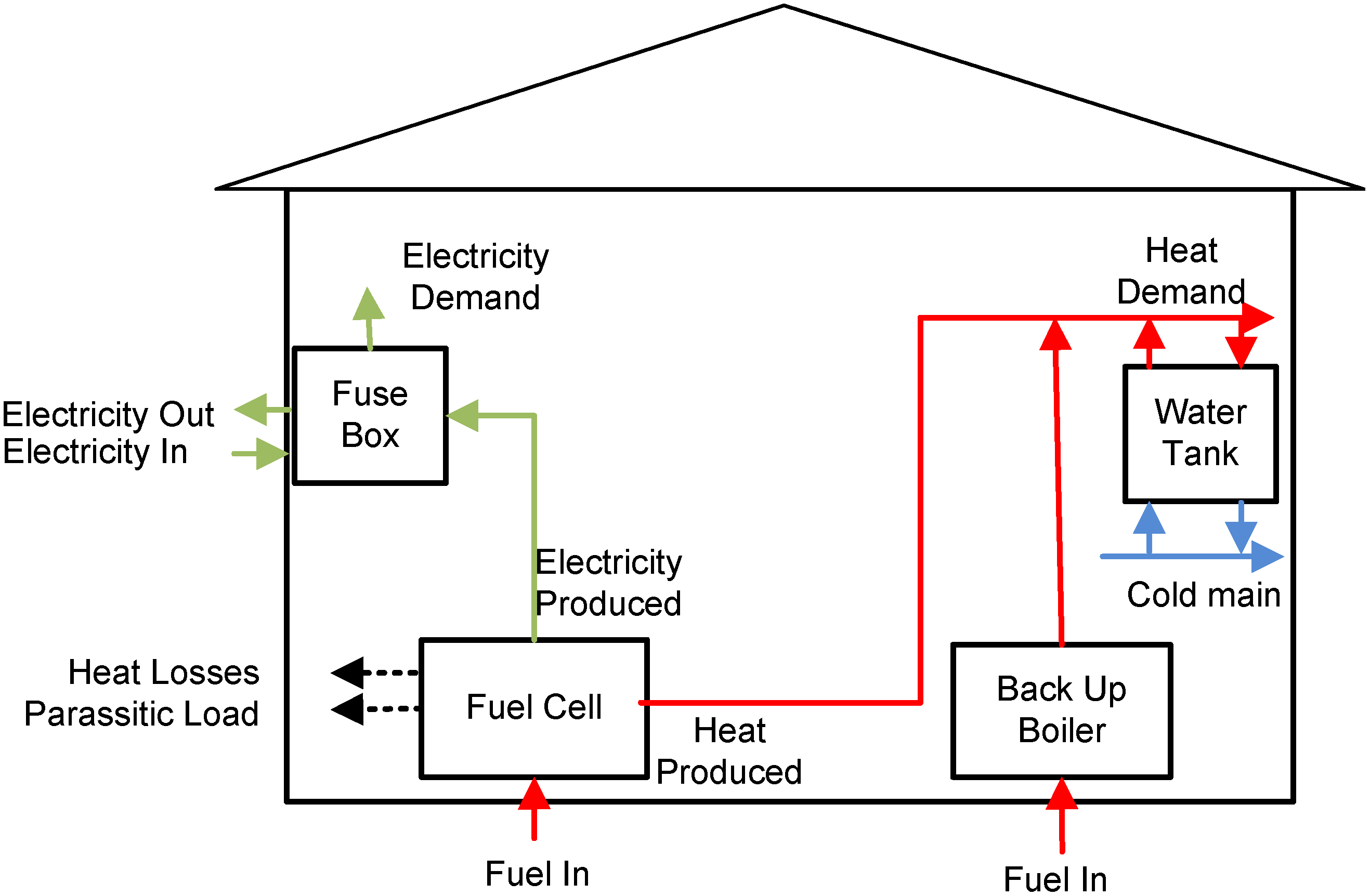
In Figure 1, a schematic of the fuel cell system coupled with a water tank for a single household is depicted. An SOFC micro-CHP unit is able to generate not only heat to support the space and water heating, but also electrical power for lightning and other electrical appliances. Furthermore, continuous operation of the micro-CHP system can reduce fuel cell degradation caused by thermal cycling and the associated mechanical stresses. There is thus a link between the operating strategy and the heat storage capacity. Although the heat-to-power ratio of a micro-CHP system can be varied when operating at different electrical loads, and through use of an auxiliary burner, there are bounds on the range of heat-to-power ratio that can be achieved [3]. Due to these limitations a storage heat tank is required in order to recover the heat produced by the system and deliver it when needed. For this reason, in this study focus is given to tank designing and sizing.

1.2. Literature Review

Many system level studies have been conducted. All of them agree that optimization results vary widely depending on different system sizing and loading conditions and thus SOFC systems should be optimized based on the specific conditions to which they are exposed (e.g., climate; household energy demand) [6,7]. SOFC systems have been combined also to absorption chillers to evaluate performance in residential applications [8]. CO₂ emissions for typical heating, cooling loads, and electricity demand profiles, for different SOFC systems to current standard technologies have been compared [9]. Besides none of these works focus on heat-to-power limitations of SOFC micro-CHP systems.

Stratified heat storage tanks have been studied mainly in solar system applications [10]. Lack of focus is given to tanks for SOFC systems in research literature. For this reason, in this study we focus on sizing a storage tank for a micro-CHP system.

Figure 1. Fuel cell system for residential application.

Figure 1. Fuel cell system for residential application.

1.3. Methodology

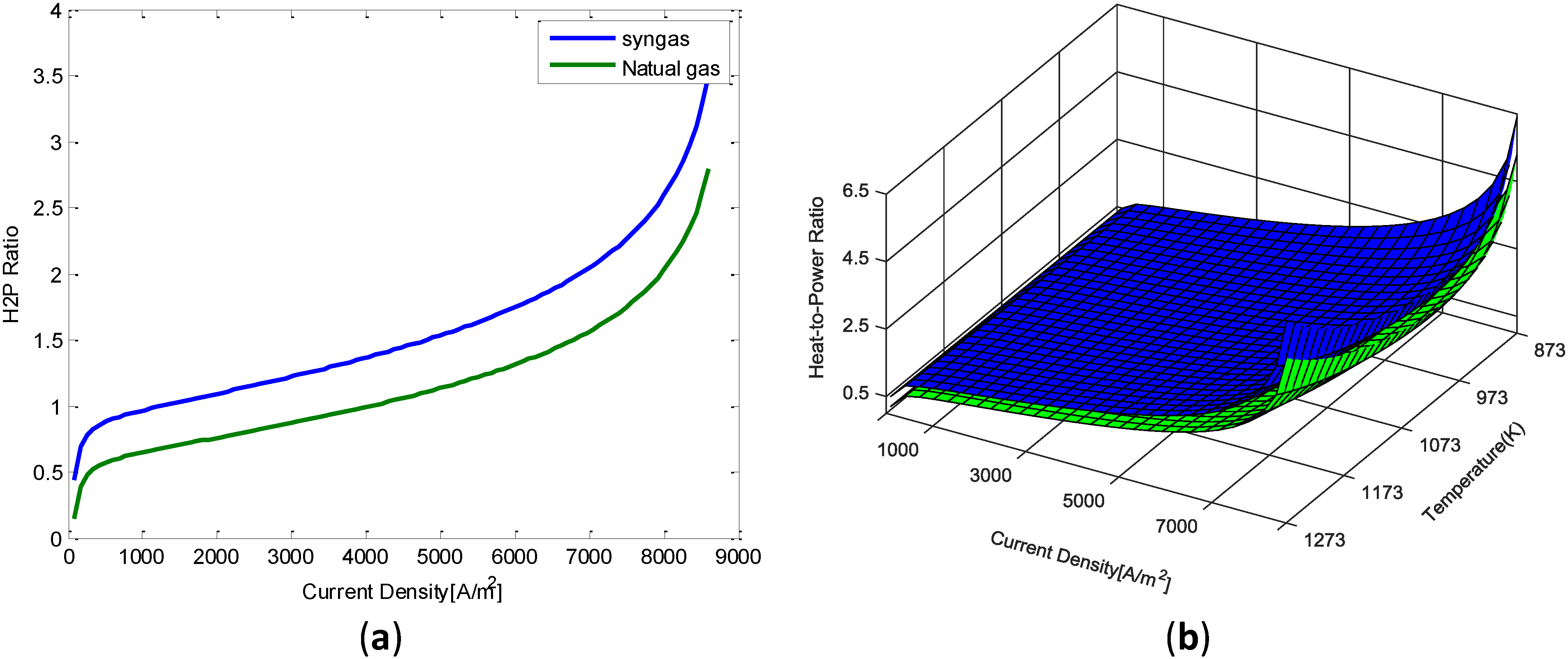
In this paper a micro-CHP system based on SOFC fuelled by syngas and natural gas is modelled. The heat-to power ratio of the systems when using two different fuels (i.e., namely syngas and natural gas) is compared. Coal-derived syngas represents an economical option given the abundance of the fuel as well as the development of gasification technology. Based on the heat recovered by the micro-CHP, a heat storage tank is sized in the two cases. Tank size is designed to ensure heat accumulation for roughly 8 h (i.e., night period). Due to low heat usage, we assume that the micro-CHP plant is operating at low heat-to-power ratio. In fact, in this period of the day the least amount of heat is requested by the household.

2. Energy System Modeling

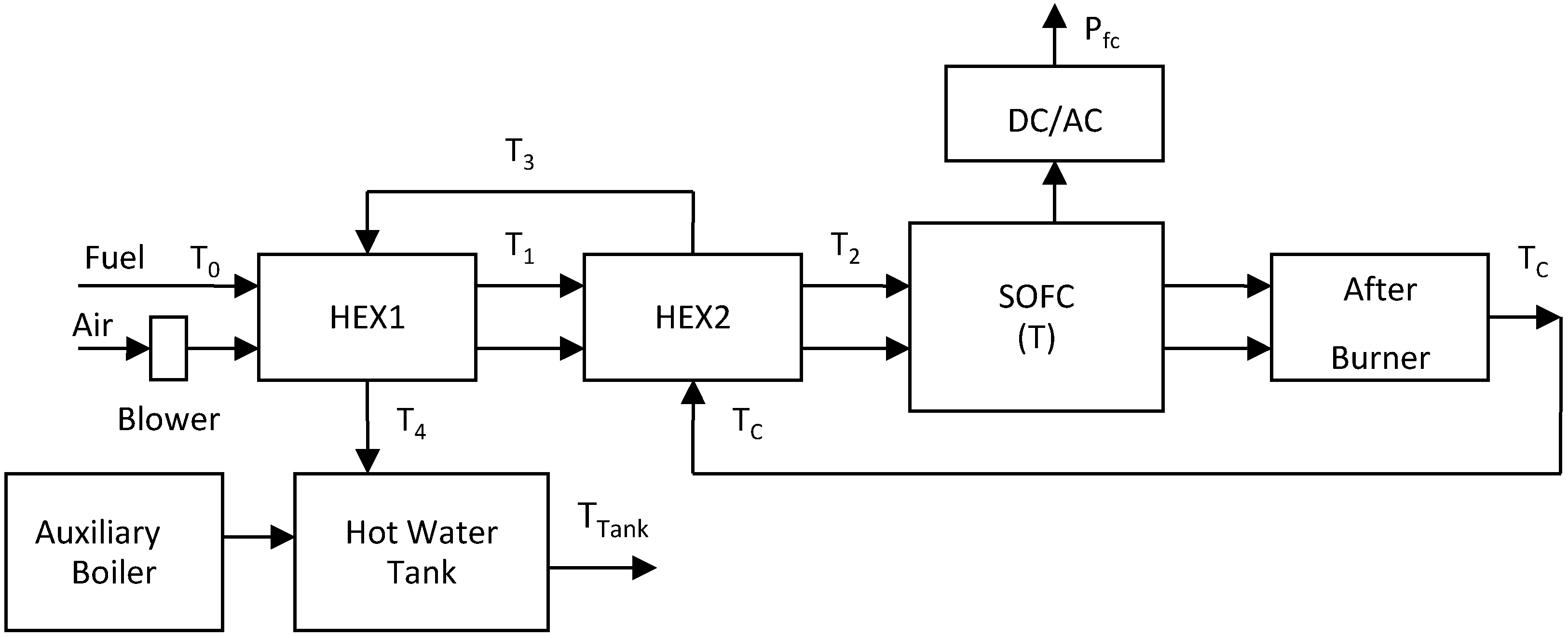
The schematic diagram of the micro-CHP system is depicted in Figure 2, where the SOFC is fuelled with syngas and coupled with a hot water tank as a heat store. Air is supplied by a blower and preheated prior to entry to the SOFC. The product gas of SOFC is sent into an afterburner, where the un-reacted fuel is burnt with part of the excess air. Fuel and air pre-heaters are required, as the fuel cell does not tolerate a gas supply at low temperatures because of the excessive cooling and consequent thermal stresses that cold streams would cause. Due to a large temperature difference between ambient and inlet fuel cell temperature (25–800 °C) hot stream is channeled in a high and low temperature heat exchanger (HEX1 and HEX2). This strategy also ensures that most of the heat is recovery.

Heat is recovered from the exhaust gas of the afterburner for preheating the inlet air and fuel before they enter the fuel cell. A hot water storage tank is used to incorporate with the fuel cell unit in order to supply hot water for the apartment with the residual heat of the exhaust gas, while extra heat can be obtained from an auxiliary boiler to cover the additional heat demand. This is an option for varying the heat-to-power ratio of the CHP system, allowing the system to cover a greater portion of domestic thermal energy demand in cold seasons.

Figure 2. Micro-CHP System model schematic.

Figure 2. Micro-CHP System model schematic.

To develop a mathematical model representing the electrochemical and thermodynamic characteristics of the entire CHP system, a number of simplifications and assumptions are made to enable the analysis:

• The fuel cell is assumed to be operated under steady-state conditions.
• The fuel cell reactions are assumed to be in equilibrium.
• Syngas consists of the following gas species, j = {H₂, CO, CH₄, CO₂, H₂O, N₂}.
• Air that enters the fuel cell consists of 79% N₂ and 21% O₂.
• The cathode and anode inlet temperature of the fuel cell are assumed to be equal.
• The cathode and anode exit temperature of the fuel cell are assumed to be equal.
• There is a temperature gradient (ΔT) across the fuel cell. The temperature of the solid structure (T) is homogeneous and midway between the inlet and exit temperatures.
• All gases behave as ideal gases.
• Gas leakage is negligible.
• Heat loss to the environment occurs only in the fuel cell.

With the help of these assumptions, the model of the micro-CHP system has been constructed and the governing equations representing all modelled components are given in the following sections. Each of the system components are modelled individually and integrated to form the overall micro-CHP system.

3. Modelling of the Micro-CHP System

3.1. Modelling the Solid Oxide Fuel Cell Fuelled with Coal Syngas

SOFCs are devices for the electrochemical conversion of a fuel gas into electrical energy. Various fuel options are feasible for SOFC operation, while coal derived syngas represents a more economical option given the abundance of the fuel as well as the development of gasification technology. The coal syngas consists primarily of hydrogen and CO, with significant water vapour and some levels of CO₂ and other minority species [11].

As commonly assumed, only H₂ oxidation is considered to contribute to the electrochemical power generation, while CH₄ is reformed to CO, which is then converted to CO₂ and H₂ through water-gas shift reaction [12,13,14]. Consequently, the steam reforming reaction for methane, the water-gas shift reaction and the electrochemical reactions occur simultaneously in the SOFC and are summarized as follows:

CH₄ + H₂O → CO + 3H₂ (reforming)

(1)

CO + H₂O → CO₂ + H₂ (water gas shift)

(2)

$${\mathrm{H}}_2+\frac{1}{2}{\mathrm{O}}_2\to {\mathrm{H}}_2\mathrm{O} \text{(overall cell reaction)}$$

(3)

A single cell model is taken as representative to simulate the SOFC, which accounts for internal reforming, and water-gas shift equilibrium, electrochemical polarizations and the associated heat generation, mass transfer via cell reactions, and overall energy balances. This representation can be readily constructed as quantities such as stack voltage and stack power which are scaled versions of single-cell voltage and power.

3.2. Mass Balance

The amount of hydrogen consumed in the fuel cell reactions, ${\dot{n}}_{{\mathrm{H}}_{2-\mathrm{c}}}$ (mol·s⁻¹), is related to the current by Faraday’s law:

$${\dot{n}}_{H_{2-c}}=\frac{iA}{n_{e}F}$$

(4)

where $i$ denotes the current density (Amp), A represents the surface area of the interconnect plate (assuming the interconnect plates have the same area), $n_e$ is the number of electrons transferred in reaction, and $F$ = 96,485 C·mol⁻¹ is Faraday’s constant. For a known fuel utilization factor, $U_f$ , the amount of hydrogen supplied, ${\dot{n}}_{{\mathrm{H}}_{2-\mathrm{s}}}$ (mol·s⁻¹), is given by:

$${\dot{n}}_{H_{2-s}}=\frac{{\dot{n}}_{H_{2-c}}}{U_f}=\frac{iA}{n_{e}F{U}_f}$$

(5)

The molar flow rate of the fuel stream needed to produce the required amount of hydrogen ${\dot{n}}_{f-in}$ (mol·s⁻¹) is thus:

$${\dot{n}}_{f-in}=\frac{{\dot{n}}_{{\mathrm{H}}_{2-\mathrm{s}}}}{x_{fc}}=\frac{iA}{n_{e}F{U}_f{x}_{fc}}$$

(6)

where $x_{fc}$ is the number of moles of hydrogen produced by 1 mol of fuel and it can be calculated according to the composition of the fuel as $x_{fc}=x_{H_2}+x_{co}+4x_{C{H}_4}$ . For a known fuel gas composition $x_j$ , its individual molar flow rate is:

$${\dot{n}}_{f-in}\left(j\right)={\dot{n}}_{f-in}{x}_j=\frac{iA{x}_j}{n_{e}F{U}_f{x}_{fc}}$$

(7)

where $j$ are the components in the fuel stream, i.e., j = {H₂, CO, CH₄, CO₂, H₂O, N₂}.

In order to avoid carbon deposition, an amount of steam equivalent to twice the amount needed for the reforming and water-gas shift reactions is supplied. The molar flow rate of steam needed, ${\dot{n}}_{H_{2}O}$ (mol·s⁻¹) is thus:

$${\dot{n}}_{H_{2}O}=({\dot{n}}_{f-in}\left(\text{CO}\right)+{\dot{n}}_{f-in}\left({\text{CH}}_4\right)\times 2)\times 2$$

(8)

The molar flow rate of additional steam supplied is thus given by:

$${\dot{n}}_{ADD}={\dot{n}}_{H_{2}O}-{\dot{n}}_{f-in}\left({\mathrm{H}}_2\mathrm{O}\right)=\left({\dot{n}}_{f-in}\left(\text{CO}\right)+{\dot{n}}_{f-in}\left({\text{CH}}_4\right)\times 2\right)\times 2-{\dot{n}}_{f-in}\left({\mathrm{H}}_2\mathrm{O}\right)$$

(9)

Therefore the total molar flow rate of the fuel stream entering the fuel cell, ${\dot{n}}_f$ (mol·s⁻¹) becomes:

$${\dot{n}}_f={\dot{n}}_{f-in}+{\dot{n}}_{ADD}$$

(10)

For known conversions for the reforming and water gas shift reactions, the component flow rates in the fuel exit stream are given as:

$$\begin{array}{c}{\dot{n}}_{f-out}\left({\mathrm{H}}_2\right)={\dot{n}}_{{\mathrm{H}}_{2-\mathrm{S}}}\times (1-U_f)\\ {\dot{n}}_{f-out}(\text{CO})=0\\ {\dot{n}}_{f-out}\left({\text{CO}}_2\right)={\dot{n}}_{f-in}\left(\text{CO}\right)+{\dot{n}}_{f-in}\left({\text{CO}}_2\right)+{\dot{n}}_{f-in}\left({\text{CH}}_4\right)\\ {\dot{n}}_{f-out}\left({\text{CH}}_4\right)=0\\ {\dot{n}}_{f-out}\left({\mathrm{H}}_2\mathrm{O}\right)=\frac{{\dot{n}}_{H_{2}O}}{2}+{\dot{n}}_{{\mathrm{H}}_{2-\mathrm{S}}}\times U_f\\ {\dot{n}}_{f-out}\left({\mathrm{N}}_2\right)={\dot{n}}_{f-in}\left({\mathrm{N}}_2\right) \end{array}$$

(11)

Given a known inlet composition, the molar flow rates for the air stream are:

$$\begin{array}{c}{\dot{n}}_{a-in}\left({\mathrm{O}}_2\right)={\dot{n}}_{{\mathrm{H}}_{2-\mathrm{S}}}\times \frac{\raisebox{1ex}{$U_f$}\!\left/ \!\raisebox{-1ex}{$2$}\right.}{U_a}\\ {\dot{n}}_{a-in}\left({\mathrm{N}}_2\right)={\dot{n}}_{a-in}\left({\mathrm{O}}_2\right)\frac{0.79}{0.21}\\ {\dot{n}}_{a-out}\left({\mathrm{O}}_2\right)={\dot{n}}_{a-in}\left({\mathrm{O}}_2\right)\times (1-U_a)\\ {\dot{n}}_{a-out}\left({\mathrm{N}}_2\right)={\dot{n}}_{a-in}\left({\mathrm{N}}_2\right)\end{array}$$

(12)

where $U_a$ is the air utilization factor, the subscript $“f”$ refers to the fuel stream, the subscript $“a”$ to the air stream, the subscript $“in”$ to the fuel cell inlet and the subscript “out” the fuel cell outlet.

3.3. Electrochemical Descriptions

The theoretical open-circuit voltage (volts) of an SOFC can be determined by the Nernst equation given as follows [15,16,17,18]:

$$E=\frac{-\mathrm{\Delta }g(T,P)}{n_{e}F}$$

(13)

Note that the molar Gibbs free energy change for the SOFC reaction depends dramatically on the temperature, T (K), and partial pressures of reactants, P, (atm), i.e., $\mathrm{\Delta }g\left(T,P\right)=\mathrm{\Delta }g°\left(T\right)-RT\text{ln}(p_{H_2}{p}_{O_2}^{\raisebox{1ex}{$1$}\!\left/ \!\raisebox{-1ex}{$2$}\right.})$ , where R = 8.314 J·mol⁻¹·K⁻¹ is the universal gas constant, $\mathrm{\Delta }g°\left(T\right)=\mathrm{\Delta }h°-T\mathrm{\Delta }s°$ stands for the molar Gibbs free energy change at $p_0=1\text{ atm}$ which also depends on temperature [15,16,17,19], $p_{{\mathrm{H}}_2}$ , $p_{{\mathrm{O}}_2}$ and $p_{{\mathrm{H}}_2\mathrm{O}}$ are the partial pressures of reactants H₂, O₂, and H₂O, respectively.

The Nernst potential is the maximum reversible voltage of an SOFC at given conditions, however the voltage of an operating SOFC is generally lower than this. As current is drawn from the fuel cell, the voltage falls due to internal resistances and overpotential losses. These losses are common to all types of fuel cells and cannot be eliminated [17,18]. Therefore, three types of polarizations, i.e., activation, ohmic and concentration, are considered and calculated through Equations (14)–(16).

(1)

Activation overpotential depends on the kinetics of the electrochemical reactions occurring at the anode and cathode. According to the general Butler-Volmer equation, the respective activation overpotentials of the anode and cathode can be calculated as:

$$\begin{array}{c}{V}_{act,a}=\frac{2RT}{n_{e}F}{\text{sinh}}^{-1}(\frac{i}{2i_{0,a}})\\ V_{act,c}=\frac{2RT}{n_{e}F}{\text{sinh}}^{-1}(\frac{i}{2i_{0,c}})\end{array}$$

(14)

where $i_{0,a/c}$ denotes the anode/cathode exchange current density.

(2)

Ohmic overpotential is caused mostly by resistance to conduction of ions and electrons and by contact resistance between the fuel cell components. In the present study, Ohmic losses are simulated as follows assuming a series electrical scheme:

$$\begin{array}{c}{V}_{ohm}=I{{\displaystyle \sum }}^{ }{R}_k=iA{{\displaystyle \sum }}^{ }\frac{L_k}{{\mathrm{\sigma }}_{k}A}=i{{\displaystyle \sum }}^{ }\frac{L_k}{{\mathrm{\sigma }}_k}=i(\frac{L_e}{{\mathrm{\sigma }}_e}+\frac{L_a}{{\mathrm{\sigma }}_a}+\frac{L_c}{{\mathrm{\sigma }}_c}+\frac{L_{int}}{{\mathrm{\sigma }}_{int}})V_{act,c}=\frac{2RT}{n_{e}F}{\text{sinh}}^{-1}(\frac{i}{2i_{0,c}})\\ {\mathrm{\sigma }}_e=C_{1e}\text{exp}(C_{2e})\\ {\mathrm{\sigma }}_a=\frac{C_{1a}}{T}\text{exp}(\frac{C_{2a}}{T})\\ {\mathrm{\sigma }}_c=\frac{C_{1c}}{T}\text{exp}(\frac{C_{2c}}{T})\\ {\mathrm{\sigma }}_{int}=\frac{C_{int}}{T}\text{exp}(\frac{C_{int}}{T})\end{array}$$

(15)

where $R_k$ represents the resistance, $L_k$ the thickness, $A$ the area, and ${\mathrm{\sigma }}_k$ denote the electronic conductivity of the anode, cathode, interconnect and the ionic conductivity of the electrolyte. $C_{1ent}-C_{int}$ are constants listed in Table 1. The subscripts a, c, e and int denote anode, cathode, electrolyte and interconnect, respectively.

Table 1. Constants used for the fuel cell model.

Parameter	Symbol	Value
Ambient temperature $(K)$	$T_0$	298
Operating pressure $(atm)$	$p_0$	1
Fuel utilization	$U_{\text{f}}$	0.8
Air utilization	$U_a$	0.2
Number of electrons	$n_e$	2
Ade exchange current density $(A{m}^{-2})$	$i_{0,a}$	6500
Cathode exchange current density $(A{m}^{-2})$	$i_{0,c}$	2500
Limiting current density $(A{m}^{-2})$	$i_L$	9000
Anode thickness $(\mathrm{\mu }m)$	$La$	500
Anode conductivity constants	$C_{1a}; C_{2a}$	95 × 106; −1150
Cathode thickness $(\mathrm{\mu }m)$	$Lc$	50
Cathode conductivity constants	$C_{1c}; C_{2c}$	42 × 106; −1200
Electrolyte thickness $(\mathrm{\mu }m$	$Le$	10
Electrolyte conductivity constants	$C_{1e}; C_{2e}$	3.34 × 104; −10,300
Interconnect thickness (cm)	$L_{int}$	0.3
Interconnect conductivity constants	$C_{1int}; C_{2int}$	9.3 × 106; −1100
Air blower power consumption factor	${\mathrm{\eta }}_{ab}$	10%

Table 1. Constants used for the fuel cell model.

Parameter	Symbol	Value
Ambient temperature $(K)$	$T_0$	298
Operating pressure $(atm)$	$p_0$	1
Fuel utilization	$U_{\text{f}}$	0.8
Air utilization	$U_a$	0.2
Number of electrons	$n_e$	2
Ade exchange current density $(A{m}^{-2})$	$i_{0,a}$	6500
Cathode exchange current density $(A{m}^{-2})$	$i_{0,c}$	2500
Limiting current density $(A{m}^{-2})$	$i_L$	9000
Anode thickness $(\mathrm{\mu }m)$	$La$	500
Anode conductivity constants	$C_{1a}; C_{2a}$	95 × 106; −1150
Cathode thickness $(\mathrm{\mu }m)$	$Lc$	50
Cathode conductivity constants	$C_{1c}; C_{2c}$	42 × 106; −1200
Electrolyte thickness $(\mathrm{\mu }m$	$Le$	10
Electrolyte conductivity constants	$C_{1e}; C_{2e}$	3.34 × 104; −10,300
Interconnect thickness (cm)	$L_{int}$	0.3
Interconnect conductivity constants	$C_{1int}; C_{2int}$	9.3 × 106; −1100
Air blower power consumption factor	${\mathrm{\eta }}_{ab}$	10%

(3)

Concentration overpotential is the voltage drop due to mass transfer limitations from the gas phase into and through the electrode. In the present study, the calculation of concentration overvoltage is as follows:

$$\begin{array}{c}{V}_{conc,a}=\frac{RT}{n_{e}F}\text{ln}(1-\frac{i}{2i_{L,a}})\\ V_{conc,c}=\frac{RT}{n_{e}F}\text{ln}(1-\frac{i}{2i_{L,c}})\end{array}$$

(16)

where $i_{L,a/c}$ denotes the limiting current density of anode/cathode.

Summing up the above overpotentials, the terminal voltage of the SOFC can be obtained as follows:

$$V=E-V_{act}-V_{ohm}-V_{conc}$$

(17)

where the expression $\text{ of }{d}_1$ is given in the Appendix.

3.4. Air Blower

In order to overcome the pressure drop in the fuel cell stack as well as to drive the air through the system, blower is needed in the SOFC section to provide motive force to the incoming atmospheric air. The electrical power required to drive this component is typically one of the largest parasitic loads for the SOFC section, and one that, if not carefully designed to meet the external power demand, can lower the overall system efficiency. A simple blower model is thus derived as follows to determine the power required for blowing air in the SOFC:

$$P_{ab}=P_{fc}{\mathrm{\eta }}_{ab}$$

(18)

where $P_{ab}$ accounts for the parasitic electrical consumption in the air blower covered by the electricity generated by the SOFC, while ${\mathrm{\eta }}_{ab}$ , the power consumption factor, is defined as a ratio of the power provided by the SOFC itself for air blowing to the total amount of power generated by the SOFC, and its value is normally no more than 20% [19,20].

3.5. Combustor

Normally only part of the fuel can be oxidized in the fuel cell, an afterburner is thus required to combust the residuals and produce additional thermal energy for use elsewhere in the system. The role of the combustor in the micro-CHP is to burn the non-reacted hydrogen coming out on the anode of the fuel cell with the non-reacted oxygen exiting the cathode. Based on the mass and energy balance of the combustor a model is developed to determine the flow-rate and temperature of the combustor exit stream, given known values for the inlet streams:

$$\begin{array}{c}{\dot{n}}_{c-out}\left({\mathrm{H}}_2\right)=0\\ {\dot{n}}_{c-out}\left(\text{CO}\right)=0\\ {\dot{n}}_{c-out}\left({\text{CO}}_2\right)={\dot{n}}_{f-out}\left({\text{CO}}_2\right)\\ {\dot{n}}_{c-out}\left({\text{CH}}_4\right)=0\\ {\dot{n}}_{c-out}\left({\mathrm{H}}_2\mathrm{O}\right)={\dot{n}}_{f-out}\left({\mathrm{H}}_2\mathrm{O}\right)+{\dot{n}}_{f-out}\left({\mathrm{H}}_2\right)\\ {\dot{n}}_{c-out}\left({\mathrm{N}}_2\right)={\dot{n}}_{f-out}\left({\mathrm{N}}_2\right)+{\dot{n}}_{a-out}\left({\mathrm{N}}_2\right)\\ {\dot{n}}_{c-out}\left({\mathrm{O}}_2\right)={\dot{n}}_{a-out}\left({\mathrm{O}}_2\right)-\frac{{\dot{n}}_{f-out}\left({\mathrm{H}}_2\right) }{2}\end{array}$$

(19)

Given all flow-rates, the temperature of the combustor exit stream $T_c$ can be further determined by solving the energy balance equation of the combustor:

$${\dot{H}}_{f-out}(T_{f-out})+ {\dot{H}}_{a-out}\left(T_{a-out}\right)={\dot{H}}_{c-out}(T_c)$$

(20)

where $T_{f-out}=T_{a-out}=T+\mathrm{\Delta }T/2.$ Equation (20) implies that the exit temperature of the combustor $T_c$ is a function of the SOFC operating temperature.

3.6. Energy Balance

Assuming ideal gas behavior, the enthalpy of a stream can be calculated as a function of the molar flow rates and temperature by [13]:

$$\dot{H}={\displaystyle \sum }_i{\dot{n}}_i{h}_i\left(T\right)={\displaystyle \sum }_i{\dot{n}}_i\mathrm{\Delta }{h}_i°+{\int }_{T_0}^T{c}_{p,i}dT$$

(21)

where the molar enthalpy of each species $i$ in the stream, $h_i\left(T\right)$ , is given as a function of the local temperature, with $\mathrm{\Delta }{h}_i°$ being the standard enthalpy change of formation of species i (J·mol⁻¹) and ${\mathrm{c}}_{\mathrm{p},\mathrm{i}}$ denoting the heat capacity of component i (J·mol⁻¹·K⁻¹). The total enthalpy change for the SOFC section is therefore determined as:

$$\mathrm{\Delta }\dot{H}=\left(-\mathrm{\Delta }{\dot{H}}_{preheater}\right)+\mathrm{\Delta }{\dot{H}}_{SOFC}=\frac{iA}{n_{e}F}\left(-\mathrm{\Delta }{h}_{preheater}+\mathrm{\Delta }{h}_{SOFC}\right)=\frac{iA}{n_{e}F}\mathrm{\Delta }h$$

(22)

where $\mathrm{\Delta }{\dot{H}}_{preheater}$ represents the enthalpy change of the endothermic preheating process, and $\mathrm{\Delta }{\dot{H}}_{SOFC}$ denotes the enthalpy change for the overall exothermic electrochemical reaction. $\mathrm{\Delta }h=-\mathrm{\Delta }{h}_{preheater}+\mathrm{\Delta }{h}_{SOFC}$ , where $\mathrm{\Delta }{h}_{preheater}$ and $\mathrm{\Delta }{h}_{SOFC}$ are expressions given in Appendix.

Considering the overpotential losses yields the rate of the total entropy production of the SOFC:

$${\dot{S}}_{tot}=\frac{I(V_{act}+V_{ohm}+V_{conc})}{T_0}$$

(23)

where $T_0$ is the ambient temperature. Based on Equation (23), the net power output of the SOFC is deduced as a function of current density, temperature, partial pressures, chemical composition, and geometric/material characteristics as:

$$P_{fc}=-\mathrm{\Delta }\dot{G}-T_0{S}_{tot}-P_{ab}=\frac{iA(-\mathrm{\Delta }g-RT{d}_1)}{n_{e}F(1+{\eta }_{ab})}$$

(24)

In terms of the efficiency, it is defined as the power output divided by the total energy input of the SOFC:

$${\eta }_{fc}=\frac{P_{fc}}{-\mathrm{\Delta }\dot{H}}=\frac{-\mathrm{\Delta }g-RT{d}_1}{-\mathrm{\Delta }h(1+{\eta }_{ab})}$$

(25)

3.7. Modelling the Heat Exchangers

As illustrated in Figure 2, two heat exchangers ( $HEX1$ and $HEX2$ ) are adopted as pre-heaters to recycle the waste heat of the system and preheat the fuel cell incoming reactants in two steps, which are modelled as flat plate counter flow heat exchangers. According to Newtonian heat-transfer and the expression of log mean temperature difference (LMTD), the heat transfer rates for the counter-flow heat exchanger $HEX1$ and $HEX2$ can be expressed as:

$$\begin{array}{c}{\dot{Q}}_{HEX1}=\dot{m}{C}_p\left(T_1-T_0\right)=U_1{A}_1\frac{\left(T_3-T_1\right)-\left(T_4-T_0\right)}{\text{ln}\frac{T_3-T_1}{T_4-T_0}}\\ {\dot{Q}}_{HEX2}=\dot{m}{C}_p[(T-\frac{\mathrm{\Delta }T}{2})-T_1]=U_2{A}_2\frac{[T_C-\left(T-\frac{\mathrm{\Delta }T}{2}\right)]-\left(T_3-T_1\right)}{\text{ln}\frac{T_C-(T-\frac{\mathrm{\Delta }T}{2})}{T_3-T_1}}\end{array}$$

(26)

where $\dot{m}$ and $C_p$ denote, respectively, the mass flow rate and heat capacity at constant pressure of the working fluid in the heat exchangers, $U_1$ and $U_2$ are the heat transfer coefficients of $HEX1$ and $HEX2$ , $A_1$ and $A_2$ represent the corresponding heat transfer surface areas.

Comparison of Equation (26) yields the following relation:

$$\frac{(T-\frac{\mathrm{\Delta }T}{2})-T_1}{T_1-T_0}=b\cdot \frac{\left[T_C-\left(T-\frac{\mathrm{\Delta }T}{2}\right)\right]-(a-1)T_1}{\left(a-1\right)T-(T_4-T_0)}\cdot \frac{\text{ln}\frac{(a-1)T_1}{T_4-T_0}}{\text{ln}\frac{T_C-(T-\frac{\mathrm{\Delta }T}{2})}{(a-1)T_1}}$$

(27)

where $a=T_3/T_1$ and $b=(U_2{A}_2)/(U_1{A}_1)$ are two parameters representing temperature ratio and heat transfer performance of the two heat exchangers. Equation (27) indicates that $T_1$ is a function of $T_3$ when other parameters are given. The values of four parameters $U_1$ , $U_2$$A_1$ and $A_2$ are not defined since an independent parameter $b$ was introduced to simplify the calculation of heat transfer performance.

Apart from heat exchangers, other irreversibilities such as heat loss from the SOFC directly to the environment cannot be neglected. In the present study, heat loss is modelled based on the temperature difference between the SOFC and ambient conditions [21]:

$${\dot{Q}}_{loss}=K{A}_l(T-T_0)$$

(28)

where $K$ denotes the effective convective and/or conductive heat-leak coefficient, and $A_l$ represents the effective heat-transfer area. Note that this equation captures the effects of fuel cell temperature changes. A detailed explanation and definition of these parameters can be found in our previous publication [22,23].

4. Micro-CHP Heat-to Power Ratio Performance

For the purpose of the work in this paper, only the micro-CHP system heat-to-power ratio with two different fuels is analyzed, namely Syngas and natural gas. We define the micro-CHP heat-to-power ratio, $H2P Ratio$ , as the ratio between the heat output, $\dot{Q}$ (Watt), and electricity output, $P_{el}$ (Watt), of the micro-CHP system [17,18]:

$$H2P Ratio=\frac{\dot{Q}}{P_{el}}$$

(29)

Micro-CHP fuel compositions for Syngas and natural gas are provided in Table 2.

Table 2. Syngas and natural gas composition.

Species	Molar Fraction
	Syngas	Natural Gas
H2	0.293	0.0
CO	0.287	0.0
CO2	0.118	0.0024
N2	0.030	0.0421
H2O	0.272	0
CH4	0.000	0.9488

Table 2. Syngas and natural gas composition.

Species	Molar Fraction
	Syngas	Natural Gas
H2	0.293	0.0
CO	0.287	0.0
CO2	0.118	0.0024
N2	0.030	0.0421
H2O	0.272	0
CH4	0.000	0.9488

In Figure 3, the micro-CHP system Heat-to-Power ratio against different current density is plotted. The plot is in good agreement with similar results in [2] and [15]. The Heat-to-Power Ratio in SOFC-based micro-CHP system fuelled by natural gas ranges between 0.5 and 1.5. We can see that a system fueled by natural gas produces around 30% less heat than a system fueled by syngas when operating at nominal conditions ( i.e., 3000–4000 A/m²). In fact, at 3000 A/m², a system fueled by syngas shows a $H2P Ratio$ equal to 1 whereas a system fuelled by natural gas has a $H2P Ratio$ around 0.7. We can conclude that a system fueled by syngas will have a $H2P Ratio$ range of operation between 0.8 and 1.95.

Figure 3. Heat-to-power ratio of a micro-CHP system fueled by syngas and natural gas at fixed temperature (a) and variable temperature (b).

Figure 3. Heat-to-power ratio of a micro-CHP system fueled by syngas and natural gas at fixed temperature (a) and variable temperature (b).

5. Stratified Storage Heat Tank Model Design

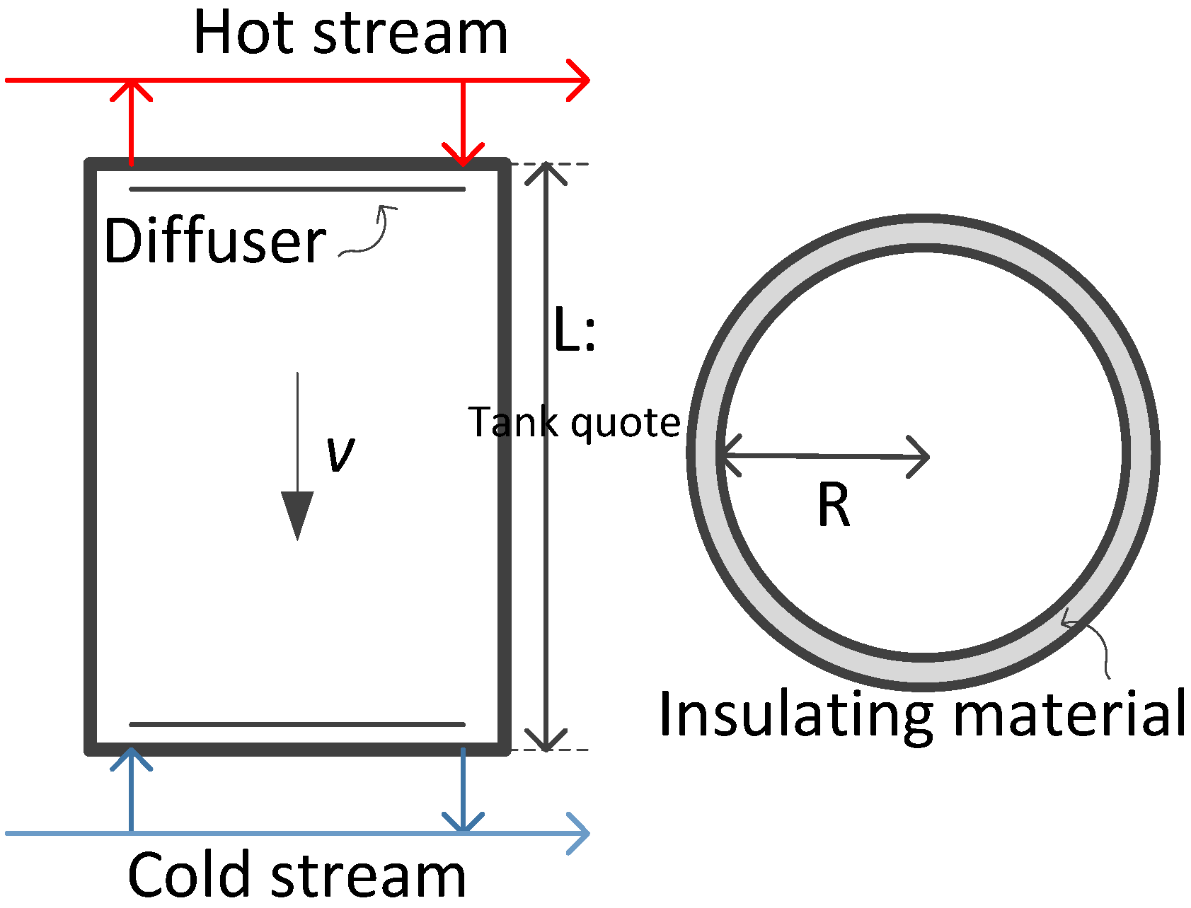
The majority of models developed for simulating thermocline storage tanks consider packed-bed systems and are based on Schumann’s one-dimensional model described in [24]. This model uses similar assumptions however it considered different heat transfer equations for fluid and packed-bed particles. A schematic of the tank with connections to the network is shown in Figure 4. Diffusers on the top and the bottom of the tank ensure equal mass flow distribution at the water inlet and outlet.

Figure 4. Schematic of the storage tank.

Figure 4. Schematic of the storage tank.

During the charging process, hot water from the micro-CHP SOFC system enters the tank from the top while cold water, extracted from the bottom, enters the returning network. The corresponding valves are open, while the others are closed. Hot water is extracted from the top and delivered to the users through the supply network. Figure 4 shows a cross section of the tank as required for the 1D numerical modeling. The energy equation applied to the general volume can be written in the form of a parabolic differential equation as follow:

$$\mathrm{\rho }{C}_{p}A\frac{\partial T}{\partial t}=\dot{m}{C}_p·\frac{\partial T}{\partial x}-h\mathrm{\psi }\left(T-T_{amb}\right)+\mathrm{\lambda }A·\frac{{\partial }^{2}T}{{\partial }^{2}x}$$

(30)

where the mass flow rate in the tank top-down direction is $\dot{m}=vA\mathrm{\rho }$ . In equation 30, $\mathrm{\rho }{C}_{p}A\frac{\partial T}{\partial t}$ represents the heat accumulation term, $\dot{m}{C}_p·\frac{\partial T}{\partial x}$ is heat carried by the flowing water, $h\mathrm{\psi }\left(T-T_{amb}\right)$ represents the heat loss through the tank insulation and $\mathrm{\lambda }A·\frac{{\partial }^{2}T}{{\partial }^{2}xt}$ is the heat transferred throughout the water volume in the tank along the vertical direction. Symbols in equation 30 are described in Table 3.

Table 3. Symbols used in Equation (30).

Symbol	Description	Constant	Unit
$x$	Distance traversed by the fluid in the tank	--	$\mathrm{m}$
$T$	Temperature of the water in the tank	--	°C
$T_{amb}$	Ambient temperature	25	°C
$\mathrm{\rho }$	Water density	990	kg·m−3
$C_p$	Heat capacity of water	4180	kj/(kg·K)
$\mathrm{A}$	Tank area	--	m2
$\mathrm{\psi }$	Tank perimeter	--	$\mathrm{m}$
$L$	Tank height	--	$\mathrm{m}$
$\dot{\mathrm{m}}$	Water mass flow rate	--	kg·s−1
$v$	Average linear velocity of water	--	m·s−1
$h$	Heat transfer coefficient of the walls	0.02	W/(m·K)
$\mathrm{\lambda }$	Thermal effective conductivity of water	0.63	W/(m·K)

Table 3. Symbols used in Equation (30).

Symbol	Description	Constant	Unit
$x$	Distance traversed by the fluid in the tank	--	$\mathrm{m}$
$T$	Temperature of the water in the tank	--	°C
$T_{amb}$	Ambient temperature	25	°C
$\mathrm{\rho }$	Water density	990	kg·m−3
$C_p$	Heat capacity of water	4180	kj/(kg·K)
$\mathrm{A}$	Tank area	--	m2
$\mathrm{\psi }$	Tank perimeter	--	$\mathrm{m}$
$L$	Tank height	--	$\mathrm{m}$
$\dot{\mathrm{m}}$	Water mass flow rate	--	kg·s−1
$v$	Average linear velocity of water	--	m·s−1
$h$	Heat transfer coefficient of the walls	0.02	W/(m·K)
$\mathrm{\lambda }$	Thermal effective conductivity of water	0.63	W/(m·K)

In this heat transfer problem, convection and radiation are only boundary conditions to conduction in solid. In we assume ambient temperature and good ventilation, convection and radiation components can be neglected.

This problem can be solved using MATLAB command $pdepe()$ , which is generally used for initial boundary value problems in one spatial dimension [25]. The matlab function accept data in the following form: $[c,f,s] = pdefun(x,t,u,dudx)$ . We consider the variable u as the temperature along the tank length. $c()$ , $f()$ and $s()$ are functions of $x, t, u$ , and du/dx where:

• x a point in the domain;
• t, the current time;
• u(), the current solution (temperature along the tank);
• du/dx(), the current solution spatial derivative.

The output to be computed by pdefun() is a set of three items:

• c(:), the coefficients of du/dt;
• f(:), the term to which d/dx is to be applied;
• s(:), the source term.

If we divide Equation (30) by the tank area A, MATLAB terms, c, f and s will be defined as follow:

$$\begin{array}{c}c=\mathrm{\rho }{C}_p\\ f=\mathrm{\lambda }·dudx\\ s=v\mathrm{\rho }{C}_p·dudx-h\mathrm{\psi }/A·(T-T_{amb})\end{array}$$

(31)

In order to solve the heat equation we must give the problem some initial conditions. So we must define the temperature of every point along the tank at time t = 0, which we do with the function $u(x,25) = u0(x)$ for $0\le x \le L$ . This function is known as the initial temperature distribution. Since heat can only enter or exit the tank at its bottom and top boundaries we must define some “boundary conditions” for the tank. Therefore we assume at the tank bottom, $u(0, t) = 25$ , and top, $u(L, t) = 60$ for all $t > 0$ . These are known as Dirichlet conditions.

The fluid effective conductivity $\mathrm{\lambda }$ specific heat $C_p$ and water density $\mathrm{\rho }$ are considered independent of temperature, being their variation negligible over the working temperature interval, 20–60 °C. The effective conductivity acts by increasing the water thermal conductivity to include turbulent mixing in the thermocline which is one of the major contributor to the loss of the thermodynamic availability of the stored energy during the charging and discharging processes. The combined effect of thermal diffusion, heat loss via the tank walls and inlet flow induced mixing was quantified by establishing an interface and allowing the thermocline to degrade over time [26,27]. Under what conditions and to what extent these assumptions are justified can be determined only by experiment. An inquiry into the experimental applications of the theory was not made in the present paper as the main purpose was to present the mathematical treatment of the problem.

6. Tank Sizing

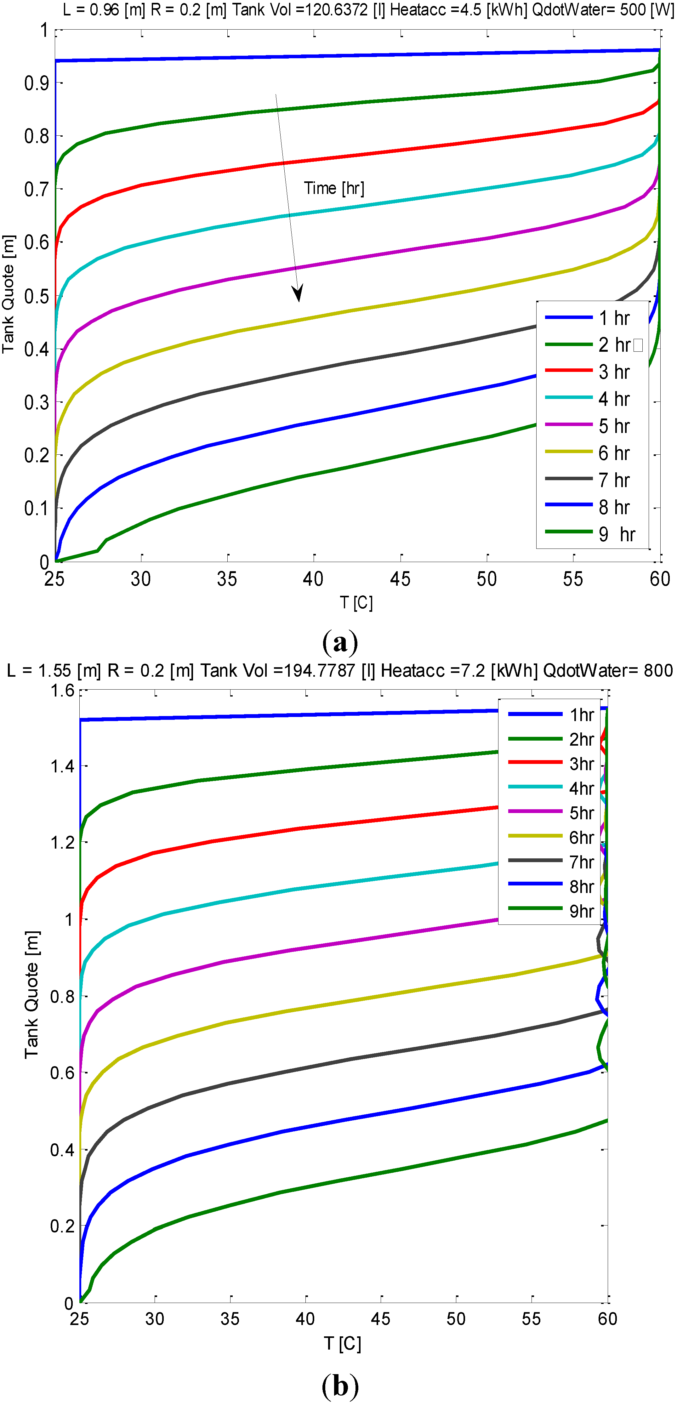
In Figure 5a,b, a temperature distribution at each hour for 9 h in tank is shown in the 2 cases studies: Micro-CHP fuelled by syngas and natural gas. Tank quote on the y-axis represents the height from the tank bottom. Water temperature is on the x-axis. Curves are plotted every hours starting from the tank top. At time = zero all the tank is at 25 °C. Hot water is charged through the inlet on the top. After one hour the code produces a linear temperature profile because the heat conduction effect is still limited. Increasing time, a larger mass of water increases its temperature and the heat conduction effect produces an s-shape temperature profile.

Water temperature distribution in the stratified tank is characterized by three regions with warm water at the top of the tank, cool water at the bottom and thermocline in the middle region. The water temperature profile over the tank height forms S-curve consisting of two asymptote curves. Average cold and warm water temperature is formed by the asymptote values of cold and hot water temperature. The position of the thermocline region defines the boundary line of cool and warm water in the tank. Thermocline degrades if the cool water depth occupied the majority of the tank volume.

In general, a thinner thermocline is desired since a larger thermocline implies a larger degradation of stratification. The thickness of the thermocline indicates the extent of mixing occurred due to inflow hot and cold streams. This factor influences the degradation of stratification as well as heat transfer losses from the tank.

Figure 5. (a) Plot of temperature distribution inside the tank in the case of micro-CHP fuelled by natural gas; (b) Plot of temperature distribution inside the tank in the case of micro-CHP fuelled by syngas.

Figure 5. (a) Plot of temperature distribution inside the tank in the case of micro-CHP fuelled by natural gas; (b) Plot of temperature distribution inside the tank in the case of micro-CHP fuelled by syngas.

Tank size was calculated to ensure heat accumulation for roughly 8 h (i.e., night period). Tank height was considered as input and it was changed so that thermocline would degrade on the ninth hour. This ensures that temperature from the top to bottom of the tank is kept in the range 60–25 °C. From Figure 5 it can be noted that in both cases, after 9 h thermocline degrades completely as the curve appears broken. This means that temperature at the bottom will be more than 25 °C after roughly 9 h of heat storage.

In order to size the tank in the two case studies the following procedure was used. Tank radius was fixed in both cases and tank volume was changed varying its height. The mCHP electric output was also fixed to one kilowatt in both cases. The inlet heat flow rate, $\dot{Q}$ , was fixed depending on the lower limit heat-to-power ratio obtained in the two cases. In the case of mCHP fueled by natural gas, it was considered 0.5 kW steady heat recovered, whereas in the case of the system fueled by syngas it was considered a steady heat recovery of 0.8 kW. This is due to the low heat use.

Water mass flow rate in the tank, $\dot{m}$ , and average linear velocity of water, $v$ , were calculated as $\dot{m}=\dot{Q}/[C_p(H2O)\cdot \mathrm{\Delta }T].$$\mathrm{\Delta }T$ represents the difference between water temperature at the main and temperature of hot water (60–20 °C). Table 4 present the designing values adopted in the two cases shown in Figure 5.

Table 4. Designing values for the tank sizing in case of mCHP fueled by natural gas and by syngas.

Value	mCHP Fueled by Natural Gas	mCHP Fueled by Syngas	Unit
mCHP electric output	1	1	kW
Lower limit heat to power ratio mCHP	0.5	0.8	–
mCHP system heat recovered mCHP	0.5	0.8	kW
Tank radius	0.2	0.2	m
Tank height	0.96	1.55	m
Tank Volume	120	194	m2
Heat Accumulation	4.5	7.2	kW
Heat flow rate	5	800	W

Table 4. Designing values for the tank sizing in case of mCHP fueled by natural gas and by syngas.

Value	mCHP Fueled by Natural Gas	mCHP Fueled by Syngas	Unit
mCHP electric output	1	1	kW
Lower limit heat to power ratio mCHP	0.5	0.8	–
mCHP system heat recovered mCHP	0.5	0.8	kW
Tank radius	0.2	0.2	m
Tank height	0.96	1.55	m
Tank Volume	120	194	m2
Heat Accumulation	4.5	7.2	kW
Heat flow rate	5	800	W

The tank sizing results give similar results to the one integrated in the micro-CHP SOFC system by CFCL BlueGen. The curve trend is in good agreement with [26,27,28]. We can see that stratification become less effective with time as the heat conduction increases.

7. Conclusions

In this paper, performance of a micro-CHP system based on SOFC where analyzed in terms of heat-to-power ratio. Two fuels were considered i.e., natural gas and syngas produced by gasification. Based on the system heat output a stratified hot water tank was sized. A detailed model of the water tank was provided in this paper. The problem of finding the temperature distributions has been solved assuming the well-known laws governing the transfer of heat from a liquid. The proposed model is useful to roughly estimate the size of the water tank.

We concluded that a system fueled by natural gas produces around 30% less heat than a system fueled by syngas when operating at nominal conditions (i.e., 3,000–4,000 A/m²). This leads to assume that a system fuelled by syngas will have a $H2P Ratio$ range of operation between 0.8 and 1.95. It was concluded that tank should able to store the heat produced by the micro CHP system when operating at the low hand of the $H2P Ratio$ for around 8 h (i.e., night period).

Finally a storage heat tank for the two cases was sized. It was shown that in the case of syngas, due to larger heat output, a larger tank volume was required in order to accumulate unused heat over the night. A 60 percent larger volume compared to the case of methane fuelled micro-CHP was estimated.