1. Introduction
Because of the concerns over climate change in recent years, the need to mitigate CO
2 emissions is increasing. Carbon capture and storage (CCS) technology is an active carbon emission reduction method that can be used to capture CO
2 from large point sources such as fossil fuel power plants (PP) or steel and cement industries and store it in geological formations. CCS is expected to serve as intermediary technology for reducing CO
2 emissions before renewable energy technologies replace the fossil fuel-based energy portfolio. Many countries are planning on reducing their CO
2 emissions using CCS technology, and 65 large-scale integrated projects are currently in operation or are being planned [
1].
In Korea, a total of 592.9 MtCO
2/year was emitted from fuel combustion in 2012, of which approximately 50% was from electricity generation [
2]. The Korean government announced a plan to reduce the country’s greenhouse gas emissions by 30% from the business as usual (BAU) level by 2020 [
3]. The BAU level represents the CO
2 emissions that would occur without any efforts at reduction. Korea suggested using CCS as the key technology for reaching its mid-term greenhouse gas reduction goals [
4]. According to the Korea CCS Plan [
4], a CCS demonstration project will start at a scale of 1 MtCO
2/year in 2017. By 2020, the CCS project will be scaled up to 3 MtCO
2/year. By 2030, CCS in Korea will expand to 32 MtCO
2/year, which corresponds to 10% of the Korea CO
2 reduction goal. Therefore, many PPs based on fossil fuel in Korea are expected to adopt CCS to meet the CO
2 emission reduction goal. Because large amounts of financial resources and additional energy consumption are needed to build and operate a CCS project, an accurate estimation of the costs before the project launch is very important.
Many studies have been carried out on the CO
2 capture costs, which constitute more than 50% of the total CCS costs. According to recent reports [
5,
6,
7], the capture costs per tonne of CO
2 for coal-fired power plants are US$50–81 for post-combustion, US$55–67 for pre-combustion and US$52–78 for oxy-fuel, respectively. For natural gas combined cycles, the costs are US$80–107 per tonne of CO
2. The CO
2 capture costs do not greatly differ for different countries or locations because they do not greatly depend on geological factors. However, the costs of transport and storage depend heavily on geographical and geological factors such as the transport distance, reservoir condition, and injection method. Therefore, it is very difficult to create general guidelines for CO
2 transportation and storage costs that can be applied to CCS projects in different countries. Important factors for the CO
2 transport costs include the transport methods, transport rates, storage sites (onshore vs. offshore), and distance. One issue of debate is whether or not ship transport is more expensive than pipeline transport. Important factors for storage costs are geological properties such as the storage capacity, injection depth, and storage sites (saline aquifer
vs. oil field, onshore
vs. offshore).
In Korea, two 10 MW-scale CO
2 capture plants are currently in the pilot test stage. The Boryeong PP is testing wet-type advanced amine technology, and the Hadong PP is testing dry-type regenerating sorbent technology [
8]. After a 1 year pilot period, the final investment decision (FID) on the construction of >100 MW CO
2 capture plants will be made. It has not yet been determined if both or just one of the CO
2 capture technologies will be selected. The Boryeong PP will have the wet-type CO
2 capture plant, and the Hadong PP or Samcheok PP will have the dry type. The potential storage site is the Ulleung Basin, which has an estimated storage capacity of 5 GtCO
2 [
9]. Only offshore storage sites are being considered as candidate storage sites because Korea is a densely populated country, and no large saline aquifer suitable for CO
2 storage has been found onshore.
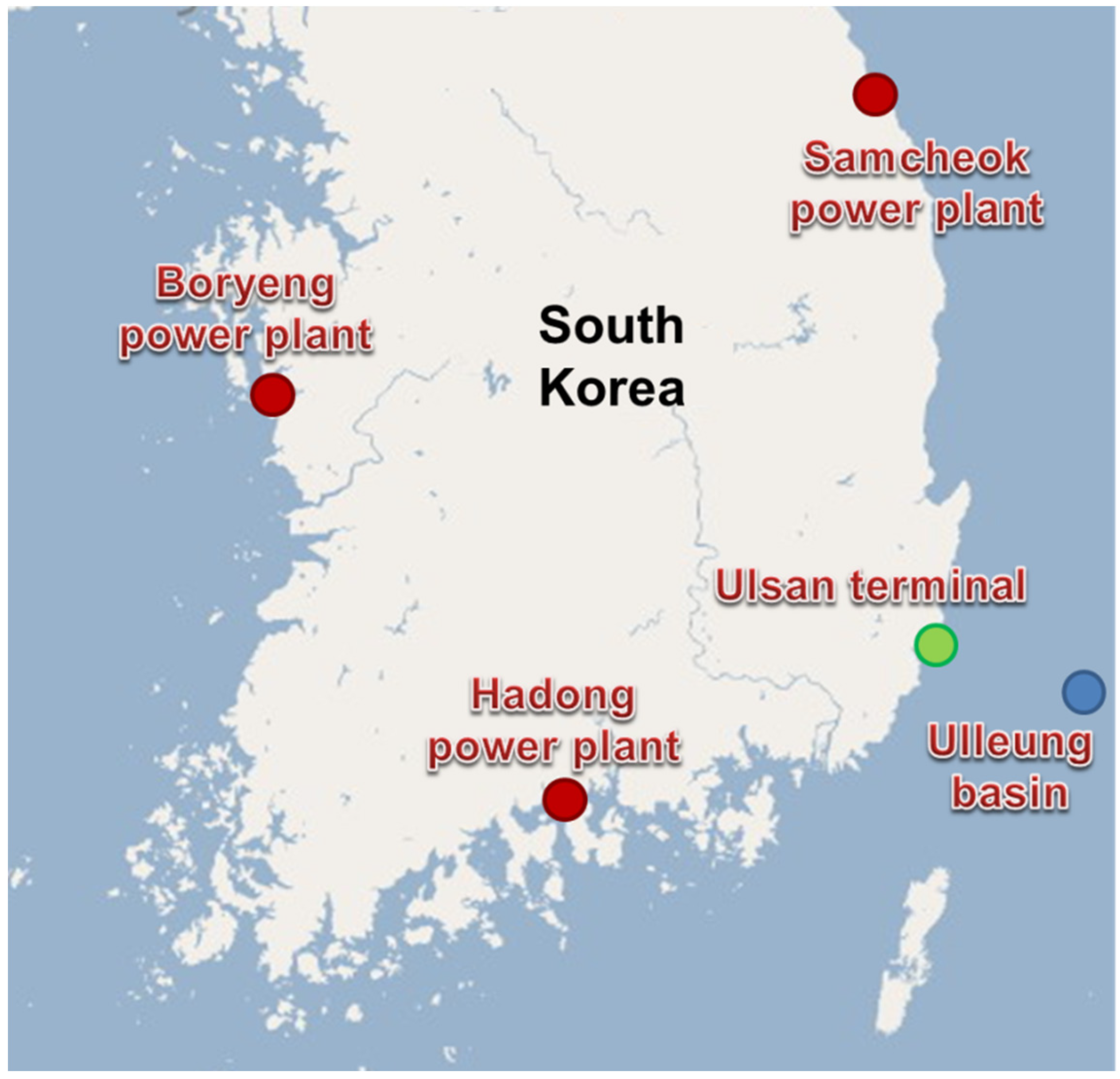
Figure 1 presents details on the locations of the three PPs and storage site. For the demonstration of the integrated CCS project, the CO
2 transport and storage systems should be set up before CO
2 capture is begun. Because the three PPs and one storage site are widely distributed around the Korean peninsula, various transport routes can be selected. Determining the optimal route is important to reaching an FID.
Figure 1.
Locations of three CO2 capture plants, CO2 hub terminal, and storage site.
Figure 1.
Locations of three CO2 capture plants, CO2 hub terminal, and storage site.
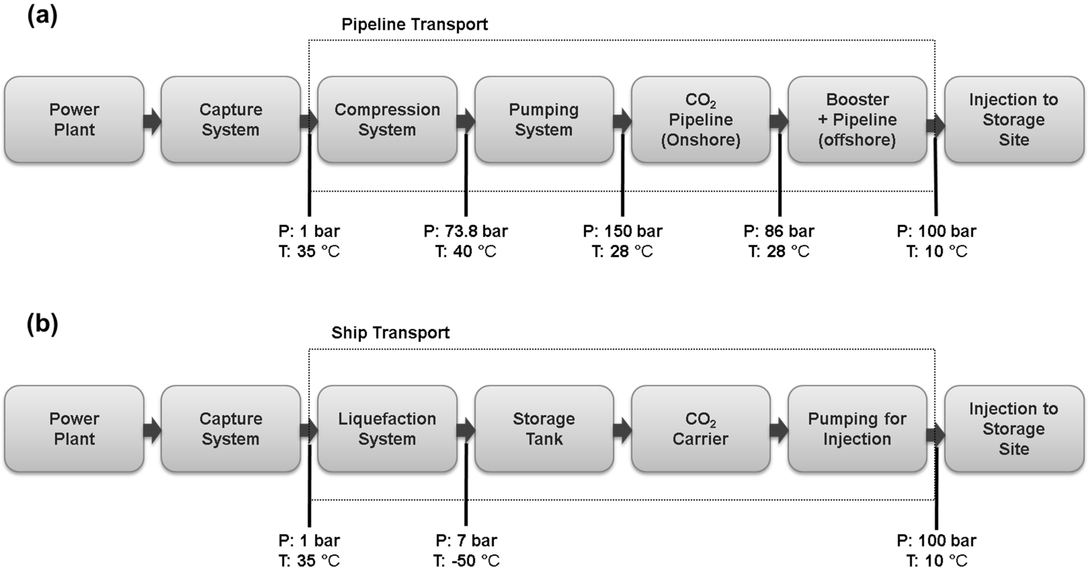
This study considered two different transport methods: a pipeline and ships. Recent studies [
10,
11,
12,
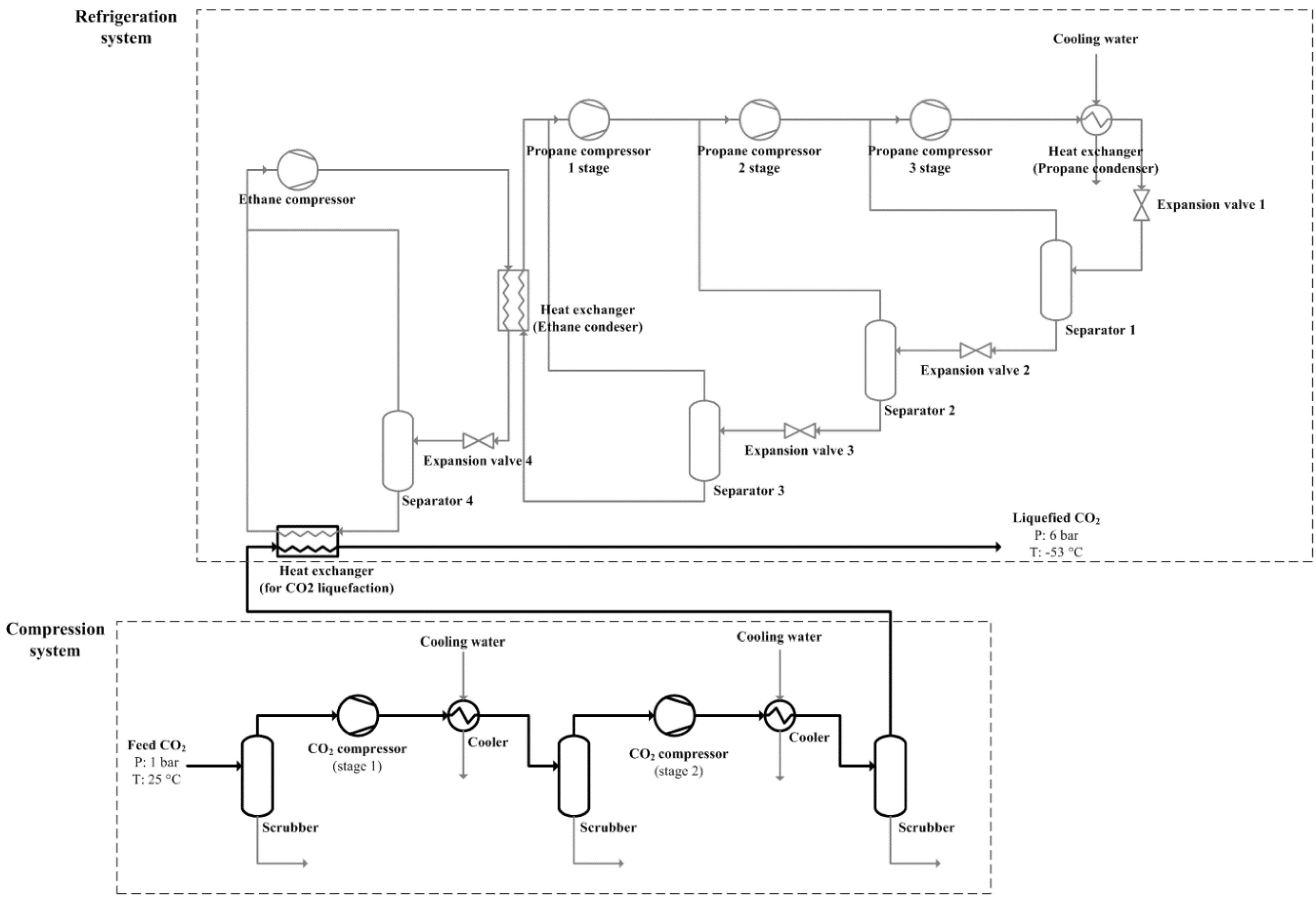
13] have reported that pipeline transport is suitable for short distances, and ship transport is suitable for long distances. The distance where ship transport becomes more cost-effective is around 200–1000 km. Because the distance from the Boryeong PP to the storage site is approximately 530 km, it is difficult to predict which method is more cost-effective. Therefore, a detailed and thorough comparison is required to determine the more cost-effective transport method. Generally, CO
2 is compressed to a level higher than the critical point for pipeline transport and is liquefied for ship transport. The costs of compression and liquefaction amount to approximately half of the total CO
2 transport costs; therefore, comparing the costs of compression and liquefaction is very critical. However, many previous studies on CO
2 transport costs did not consider the compression and liquefaction costs. Recent studies [
11,
12,
13,
14] have considered the cost of the liquefaction process, but these studies assumed that the CO
2 was already compressed to a pressure greater than 100 bar and only considered the additional liquefaction cost. To strictly compare the transport costs between pipeline transport and ship transport, the compression/liquefaction costs were considered in this study.
A techno–economic model was used to evaluate the CO2 transport costs of various cases with different transportation routes and methods. First, three different CO2 transport scenarios in Korea were set up based on the three PPs and one storage site. The pressure and temperature conditions at each stage of transport were assumed, and the lowest costs for the equipment were identified as the optimum values. The calculated costs were compared for different transport rates and methods to characterize the costs of CO2 transport in Korea.
2. CO2 Transport Scenarios
Table 1 gives the three CO
2 transport scenarios set up with different combinations of the three capture plants.
Figure 2 shows the detailed transport routes of each scenario.
Table 1.
CO2 transport scenarios.
As noted in the introduction, the wet-type and dry-type CO2 capture technologies are competitors in Korea, and it has not yet been determined whether one or both types will be selected in the FID. Because the wet-type capture is verified and mature technology, the Boryeong PP using it was included in all scenarios. The Hadong PP and Samcheok PP, which are based on dry-type technology, were included in Scenarios 2 and 3, respectively. In summary, Scenario 1 has only one capture plant (Boryeong), Scenario 2 has two capture plants (Boryeong on the west coast and Hadong in the southern part of the Korean Peninsula), and Scenario 3 has two capture plants (Boryeong and Samcheok on the east coast). The Ulleung Basin served as the fixed storage site in all of the scenarios. Scenario 3 includes the hub terminal at Ulsan, but Scenarios 1 and 2 do not.
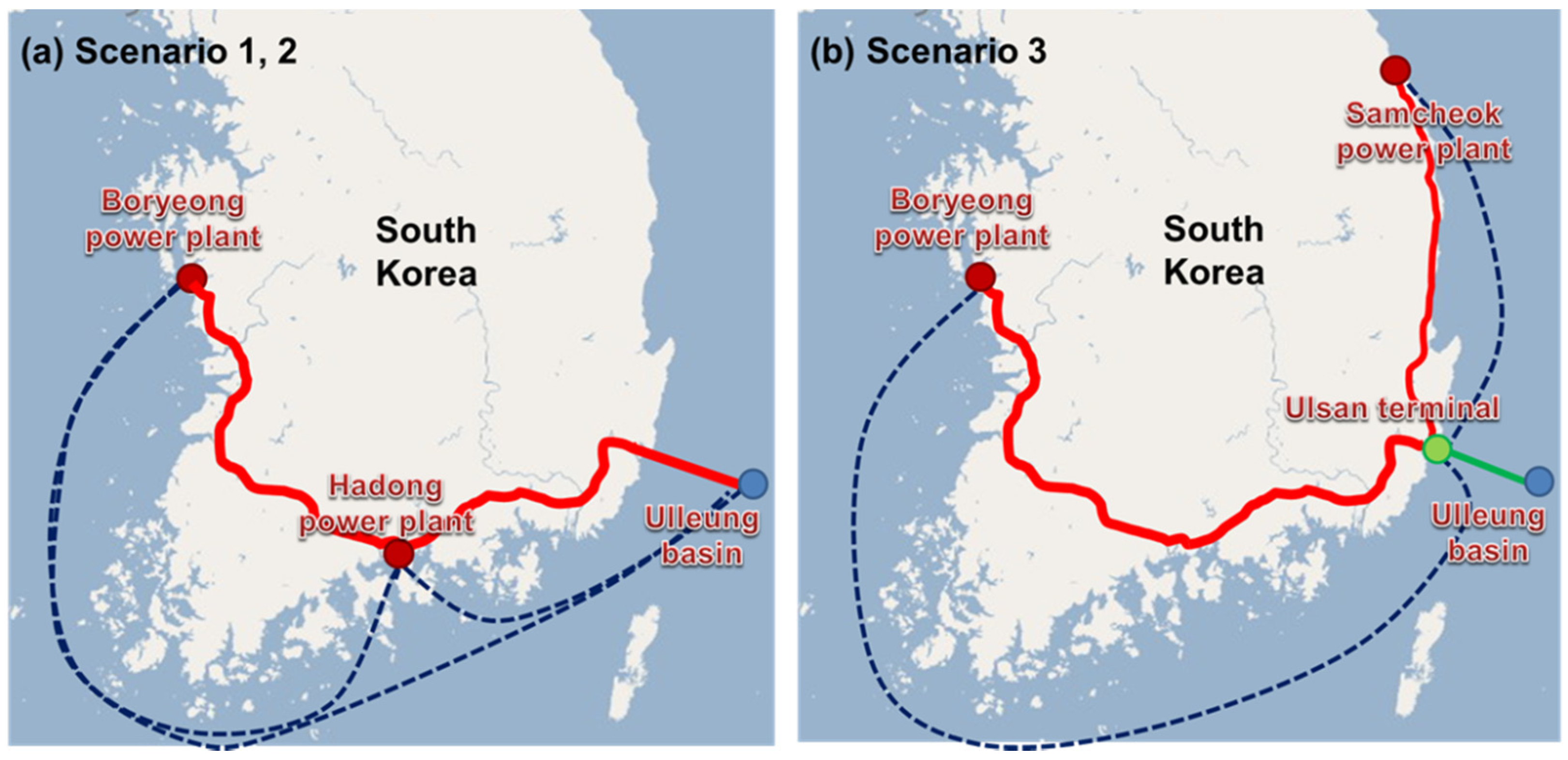
Figure 2.
CO2 transport scenarios in Korea: (a) Scenarios 1 and 2 and (b) Scenario 3. Scenario 1 has one capture plant at Boryeong, Scenario 2 has two capture plants at Boryeong and Hadong, and Scenario 3 has two capture plants at Boryeong and Samcheok. The CO2 storage site is fixed at the Ulleung Basin. Scenario 3 has a hub terminal at Ulsan, but Scenarios 1 and 2 do not. The solid red lines, solid green line, and dotted blue lines represent the onshore pipeline transport routes, offshore pipeline transport route, and ship transport routes, respectively.
The CO
2 transport volume was varied in the range of 1–6 MtCO
2/year to determine its effect; the values are summarized in
Table 1.
Table 2 lists the details of the transport distances. For the pipeline transport in Scenario 1, the transport route from the Boryeong PP to the storage site is not the shortest route but follows the plains around the coastline to avoid the high mountains in the center of the Korean peninsula, as shown in
Figure 2a. Because the Hadong PP in Scenario 2 is located on the route of Scenario 1, the pipeline transport routes of Scenario 2 are the same as the route of Scenario 1. However, in Scenario 2, CO
2 is added from the Hadong PP. In Scenario 3, the Boryeong and Samcheok PPs are included; because they are located on the west and east coasts, respectively, of the Korean peninsula (
Figure 1), the hub terminal was assumed to be set up in Ulsan harbor, which is the nearest harbor to the storage site. Scenario 3 has three different transport methods: pipeline transport for both the Boryeong PP–Ulsan Harbor and Samcheomk–Ulsan Harbor routes, ship transport on both routes, and both transport methods on both routes (
i.e., ship transport for the Boryeong PP–Ulsan Harbor route and pipeline transport for the Samcheok–Ulsan Harbor routes). Ship transport is understood to be more economical than pipeline transport for long distances. Therefore, ship transport was adopted for the longer Boryeong PP–Ulsan terminal route, and pipeline transport was adopted for the shorter Samcheok PP–Ulsan terminal route in Scenario 3, as shown in
Figure 2b. The transport method between the hub and storage site was fixed to an offshore pipeline.
Table 2.
Distances from PP (Power Plant) to PP, PPs to storage site, PPs to hub terminal, and hub terminal to storage site.
Table 2.
Distances from PP (Power Plant) to PP, PPs to storage site, PPs to hub terminal, and hub terminal to storage site.
| Departure/Destination | Pipeline (km) | Ship (km) |
|---|
| Boryeong PP to Hadong PP | 280 | 617 |
| Hadong PP to Ulsan terminal | 190 | N/A |
| Ulsan terminal to Ulleung Basin | 60 | 60 |
| Boryeong PP to Ulleung Basin | 530 | 724 |
| Boryeong PP to Ulsan terminal | 470 | 726 |
| Hadong PP to Ulleung Basin | 250 | 270 |
| Samcheok PP to Ulsan terminal | 250 | 282 |
4. Results
Figure 5,
Figure 6 and
Figure 7 show the normalized cost of each scenario for the different transport methods and transport rates. The capital recovery factor in the normalized cost was 0.08 with a repayment period of 20 years and interest rate of 5%. In the figures, the notations “Emitter”, “Onshore”, “Offshore”, “Carrier”, “Injection”, and “Hub” represent the compression or liquefaction costs in the capture plant, onshore pipeline, offshore pipeline, CO
2 carrier, pumping for injection to the storage site, and hub terminal, respectively.
On the x-axis, the letters “B”, “H”, and “S” represent the Boryeong, Hadong, and Samcheok PPs, respectively. The numbers after the letters are the transport rates (MtCO2/year). For example, “B1 + H3” denotes the capture plants at the Boyeong PP with a captured amount of 1 MtCO2/year and Hadong PP with a captured amount of 3 MtCO2/year.
Figure 5.
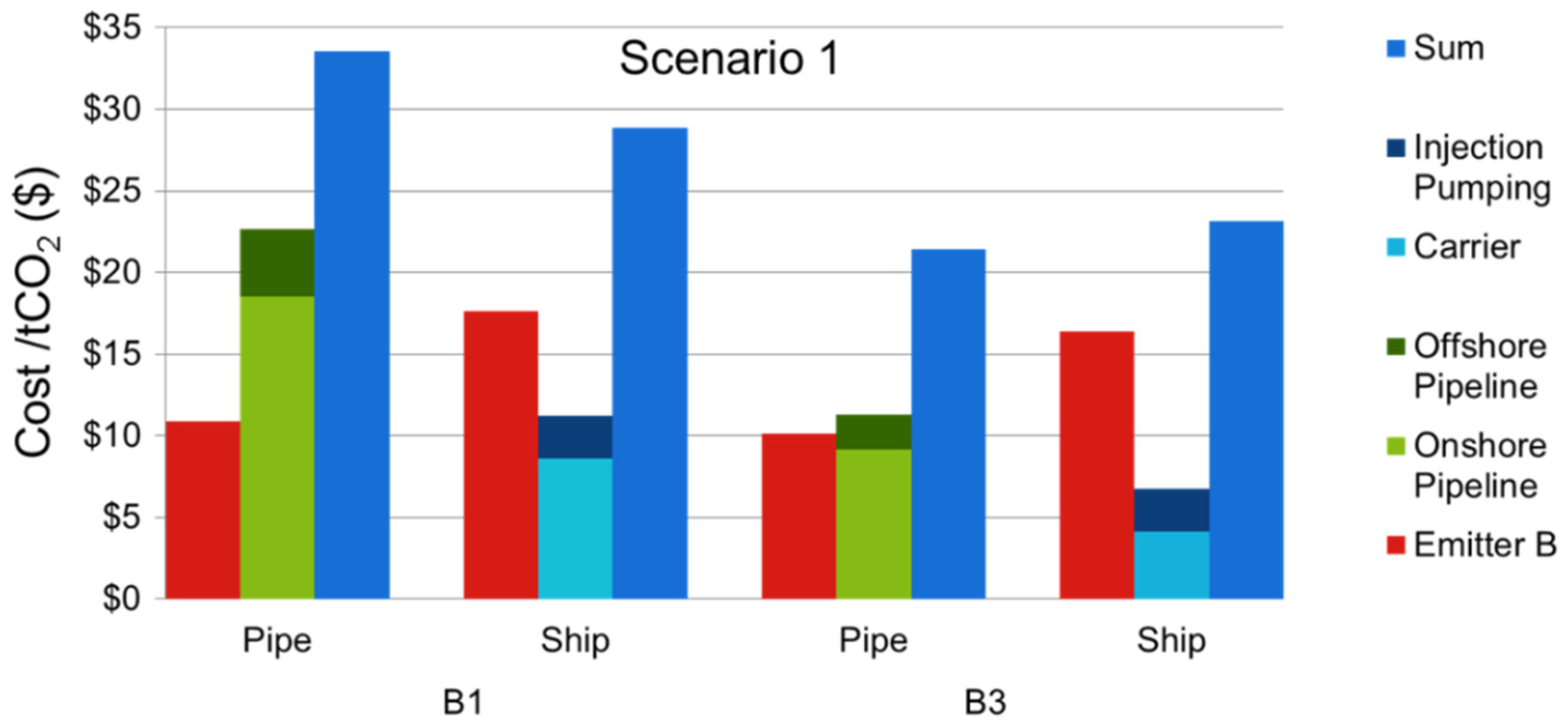
CO2 transport costs per unit tCO2 in Scenario 1.
Figure 5.
CO2 transport costs per unit tCO2 in Scenario 1.
Figure 6.
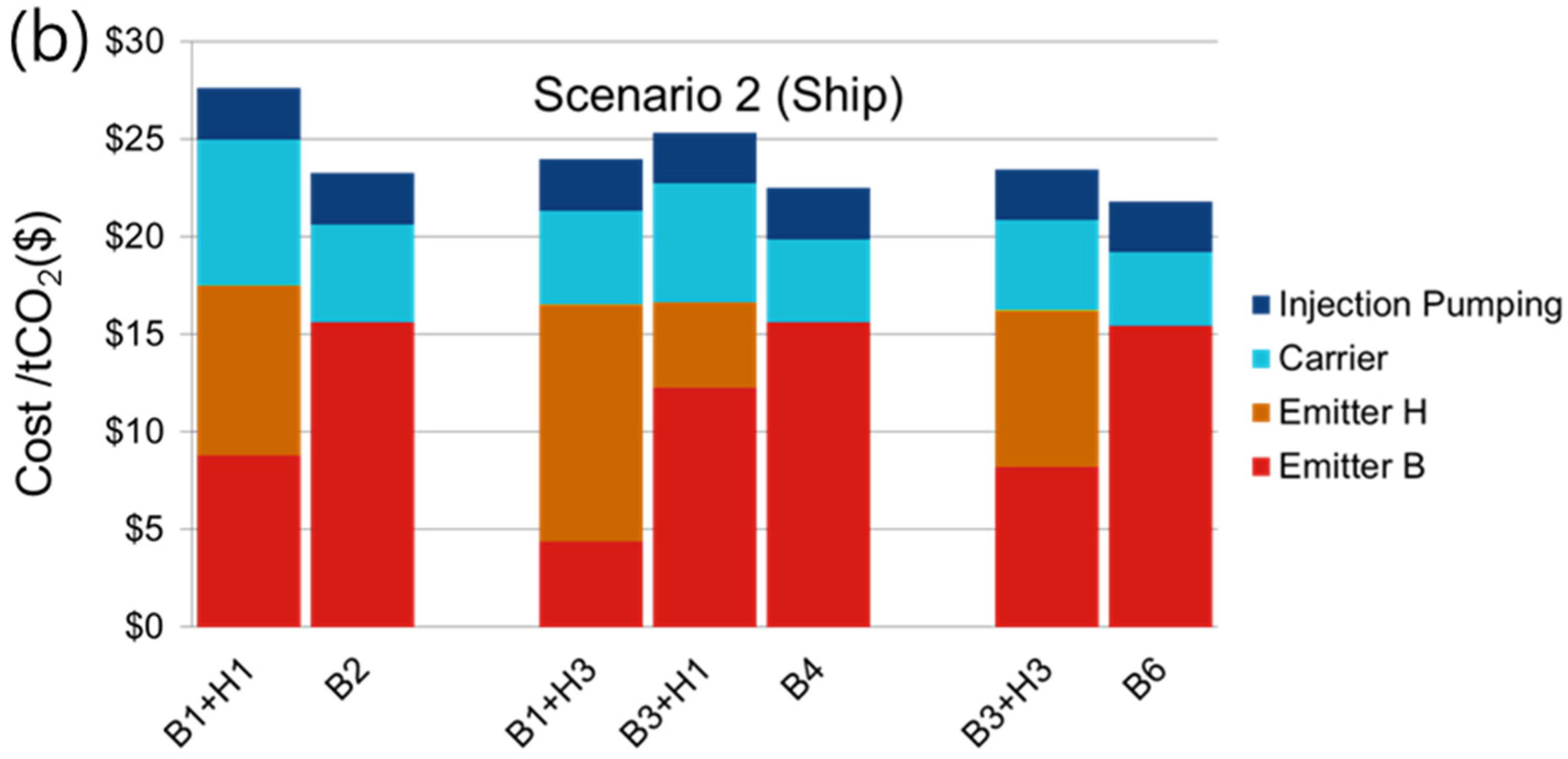
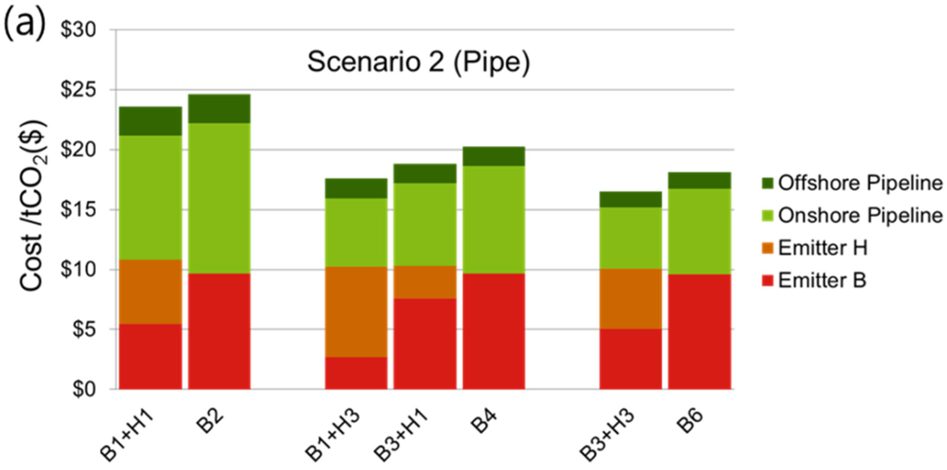
CO2 transport costs per unit tCO2 in Scenario 2: (a) pipeline transport, (b) ship transport.
Figure 6.
CO2 transport costs per unit tCO2 in Scenario 2: (a) pipeline transport, (b) ship transport.
Figure 7.
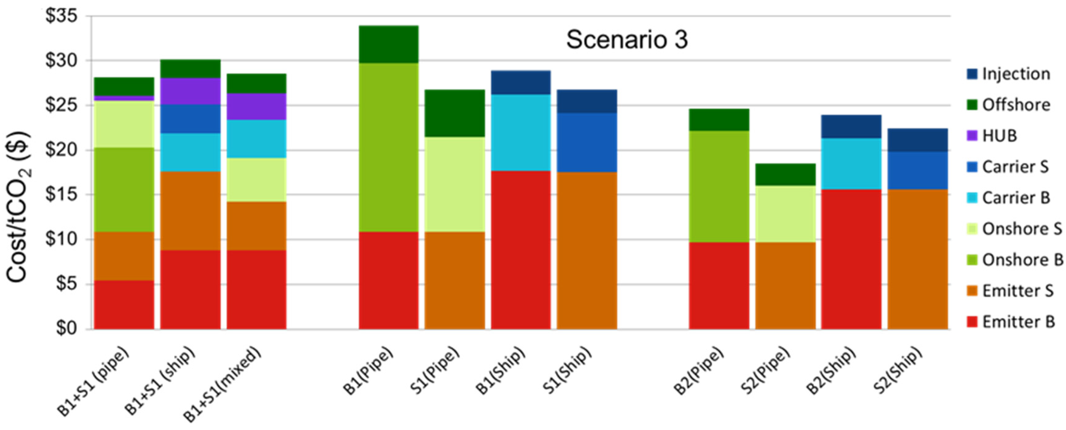
CO2 transport costs per unit tCO2 in Scenario 3.
Figure 7.
CO2 transport costs per unit tCO2 in Scenario 3.
4.1. Scenario 1
Figure 5 shows the transport cost of Scenario 1. The costs of pipeline transport at the two transport rates of 1 and 3 MtCO
2/year were compared. The compression costs of Emitter B at 1 and 3 MtCO
2/year were both approximately US$10/tCO
2 and showed little difference. The almost constant compression cost per ton of CO
2 was due to two reasons. First, an increase in the transport rate did not mean an increase in the equipment size but in the number of trains. Because the CAPEX of the compression/liquefaction costs in the emitter was proportional to the number of trains in parallel, an economies of scale effect produced by the increased capture rate was difficult to expect. Second, the most dominant factor for the emitter cost was the electric power, but the unit electric power consumption for CO
2 compression was not heavily affected by the amount of CO
2. In contrast, the costs of the onshore and offshore pipeline significantly decreased as the transport rate increased. As shown in
Figure 5, the costs of the onshore and offshore pipelines at 1 MtCO
2/year were US$18/tCO
2 and US$5/tCO
2, respectively. The costs of the onshore and offshore pipelines at 3 MtCO
2/year were about twice the costs at 1 MtCO
2/year. Unlike the emitter cost, the CAPEX was the dominant factor for the pipeline cost, and a large-diameter pipeline was cost-effective per ton of CO
2. Despite the almost constant emitter cost, the overall economies of scale effect on the pipeline cost was high because of the significant effect on the onshore and offshore pipeline costs. For example, the estimated pipeline cost at 1 MtCO
2/year of US$33/tCO
2 was reduced to US$21/tCO
2 at 3 MtCO
2/year.
When the costs of ship transport at the transportation rates of 1 and 3 MtCO2/year were compared, the emitter costs were found to remain almost constant with an increased transport rate, while the carrier costs were greatly reduced, similar to the pipeline cost. Note that the liquefaction cost was assumed to be proportional to the compression cost, and the characteristics of the emitter cost for the ship and pipeline transport methods were similar. The economies of scale effect on the carrier cost was so strong that the carrier costs at 3 MtCO2/year were around half the costs at 1 MtCO2/year. The cost of injection pumping heavily depended on the electric power consumption while being independent of the transportation rate, similar to the emitter costs.
Because the emitter costs accounted for 30%–70% of the total transport cost, the difference in emitter costs between the compression and liquefaction processes could determine which of the pipeline transport and ship transport provides the least cost. Without including the emitter costs, the ship transport method was less costly than the pipeline method at both 1 and 3 MtCO2/year. At 1 MtCO2/year without the emitter cost, the pipeline transport cost was approximately US$23/tCO2, while the ship transport cost was approximately US$11/tCO2. Because the emitter costs were independent of the transport distances and rates, the difference in emitter cost of approximately US$7/tCO2 between liquefaction and compression was fixed. Therefore, for the ship transport cost to be more cost-effective than the pipeline transport cost, the sum of the carrier and injection pumping costs had to be approximately US$7/tCO2 less than the sum of the onshore and offshore pipeline costs. At 1 MtCO2/year, the ship transport with the emitter cost was still more cost-effective than the pipeline transport. At 3 MtCO2/year, the pipeline transport with the emitter cost became more cost-effective than the ship transport. This implies that, for the strict comparison of pipeline and ship transport methods, the costs of compression/liquefaction must be included in the transport costs.
4.2. Scenario 2
Scenario 2 is an extended version of Scenario 1 that includes an additional load of CO
2 on the route.
Figure 6 shows the calculated costs of Scenario 2. As shown in
Figure 2, Scenario 2 has a similar route to Scenario 1 that starts at the Boryeong PP and ends at the Ulleung Basin; however, there is an additional CO
2 load at the Hadong PP. The effect of the additional CO
2 on the route was studied by comparing Scenarios 1 and 2. In other words, each case of Scenario 2 was compared with the case of Scenario 1, where the transport rate was the same as the sum of the captured CO
2 at the Boryeong and Handong PPs.
For pipeline transport, the distance from the Boryeong PP to the Hadong PP was 280 km, which corresponded to approximately 53% of the total distance. Because the transport rate in the Boryeong–Hadong section was less than that in the other section because of the addition of CO
2 at the Hadong PP, a large reduction in cost was expected compared to Scenario 1. However, the cost reduction in Scenario 2 was not as large as expected, as shown in
Figure 6a. There are two reasons for the small cost reduction. First, the cost reduction in the onshore pipeline induced by the lower transport rate in the Boryeong–Hadong section was ~30% because of the well-known economies of scale effect with regard to mass flows [
45]. For example, the cost of the onshore pipeline at B1 + H1 was approximately US$10/tCO
2, which corresponded to 80% of the onshore pipeline at B2, as shown in
Figure 6a. The cost of the onshore pipeline at B1 + H3 showed the largest cost reduction compared to the corresponding Scenario 1 because the difference in the transport rate between the Boryeong–Hadong section and the other section was as high as 3 MtCO
2/year. Second, the increased emitter costs from the two PPs compared to the emitter cost from the single PP in Scenario 1 offset the cost reduction in the onshore pipeline. For B1 + H1, the sum of Emitters B and H was approximately US$11/tCO
2, which was approximately US$1.5/tCO
2 higher than that of Emitter B in the B2 case. The cost of the offshore pipeline did not change between Scenarios 1 and 2 because the transport rate and other conditions were the same.
Unlike the pipeline costs of Scenario 2, the ship transport costs of Scenario 2 were higher than those of Scenario 1. In all cases of the ship transport costs, as shown in
Figure 6b, the emitter and carrier costs of Scenario 2 were higher than the costs of the corresponding cases in Scenario 1. Because the CO
2 in Scenario 2 was captured at the two PPs, the emitter costs of Scenario 2 were higher than those of Scenario 1, where CO
2 was captured at only one PP. In contrast to the pipeline costs of Scenario 2, the ship transport distances of Scenario 2 were much greater than those of Scenario 1. In Scenario 1, the ship transport distance from the Boryeong PP to the Ulleung Basin was 724 km. However, the transport distance of Scenario 2 comprised two routes from the Boryeong PP to the Hadong PP and from the Hadong PP to the Ulleung Basin. The total distance of the two routes was 877 km, which was 22% longer than the routes of Scenario 1. This increased distance in Scenario 2 increased the carrier costs compared to Scenario 1. For example, the carrier cost of B1 + H1 in
Figure 6b was approximately US$7.50/tCO
2, which was US$2.50/tCO
2 higher than the corresponding Scenario 1 case of B2. When the B2 costs for the pipeline transport method, as shown in
Figure 6a, and ship transport method, as shown in
Figure 6b, were compared, the latter was more cost-effective. However, when the B1 + H1 costs of the two transport methods were compared, the pipeline transport method was found to be more cost-effective. The different characteristics of the ship and pipeline transports in Scenario 2 indicated that the CO
2 transport cost is very sensitive to geological factors and transport conditions, which makes it difficult to set up general rules.
4.3. Scenario 3
The main difference between Scenario 3 and Scenarios 1 and 2 is the presence of the hub at Ulsan Harbor and the lack of overlapping between the two transport routes. The Boryeong and Samcheok PPs were assumed to be the CO
2 capture plants in Scenario 3, as shown in
Figure 2. Unlike Scenarios 1 and 2, the capture rate at each PP in Scenario 3 was fixed to 1 MtCO
2/year.
The costs of Scenario 3 were compared with the cases with only one capture site using both transport methods, as shown in
Figure 7. The left three columns show the costs of Scenario 3 for the different transport methods. The pipeline method showed the least cost of approximately US$28/tCO
2, but the difference in costs among the three methods was small. The costs of the hub in
Figure 7 consisted of the storage tanks and pressurization of the carrier-transported CO
2 in the offshore pipeline. The pressurization costs of the ship-transported CO
2 accounted for the largest proportion. The hub cost of the pipeline transport was very small because no pressurization process was required, so only the storage tank cost was included in this case.
The four columns on the right in
Figure 7 show the transport cost for one capture plant with no hub terminal at 2 MtCO
2/year. The transport cost of the four right columns with one capture plant and no hub terminal was much smaller than that of the three left columns with two capture plants and the hub terminal. The B1 + S1 case had two fundamental disadvantages compared to the B2 (pipe) and S2 (pipe) cases. The first was the longer transport distance. For example, the transport distances of B2 (pipe) and S2 (pipe) from the PPs to Ulsan were 470 and 250 km, respectively. However, the transport distance of B1 + S1 (pipe) from the PPs to Ulsan was the sum of 470 and 250 km. This much greater transport distance induced a higher cost for B1 + S1 (pipe) that was higher than the cost of B2 (pipe) or S2 (pipe), even though the transport rate for each route of B1 + S1 (pipe) was half the rate of B2 (pipe) or S2 (pipe). The second reason was the additional hub cost for B1 + S1.
The results of Scenario 3 are especially useful when a CO
2 transport route is added to an existing transport route. For example, assume that S1 (pipe) is already in operation, and the capture of CO
2 at the Boryeong PP is planned and needed to setup a CO
2 transport route with the same storage site as S1 (pipe). In this case, four choices are possible: (1) an extra pipeline route without a hub, (2) an extra ship route without a hub, (3) an additional pipeline route with a hub, and (4) an additional ship route with a hub. For choice 1, the cost of B1 (pipe) in
Figure 7 would additionally be required, and the total cost (per MtCO2/year) would be the average of S1 (pipe) and B1 (pipe). For choice 2, the cost of B1 (ship) would be additionally added, and the total cost (per MtCO2/year) would be the average of S1 (pipe) and B1 (ship). For choices 3 and 4, the costs would be B1 + S1 (pipe) and B1 + S1 (mixed), respectively. Choices 1 and 3 are the same in that the pipeline transport method is adopted, but they differ in the sharing of the offshore pipeline and presence of a hub. Therefore, with B1 + S1 (pipe), the sharing of the offshore pipeline and small storage tank make the cost of B1 + S1 (pipe) smaller than the average cost of B1 (pipe) and S1 (pipe). Similarly, choices 2 and 4 both adopt the ship transport method from the capture plants, but they differ in that choice 4 shares the offshore pipeline. In choice 2, the ship- and pipeline-transported CO
2 are separately transported to the storage site. Except for the temporary storage cost at the hub with choice 4, the other costs do not greatly differ. Therefore, choice 4 shows slightly higher overall costs than choice 2. However, the complexity of choice 2 with the injection may offset the hub cost of choice 4.
The hub is economically advantageous when the hub gathers CO2 from several routes and the distances from the hub to the storage site are long enough to produce the economies of scale effect. Overall, the incorporation of a hub in Scenario 3 did not result in high efficiency because of the relatively short distance from the hub to the storage site (approximately 60 km) and small number of gathered CO2 routes.
5. Conclusions
In this study, the CO2 transport costs in Korea were calculated using the techno-economic method. Three scenarios were developed that depended on the locations of the CO2 capture plants, and each scenario included both the pipeline and ship transport methods. The compression/liquefaction costs constituted a large portion of the total transport cost. The economies of scale effect was significant on both the carrier cost and costs of the onshore and offshore pipelines, but it was negligible on the compression/liquefaction costs. Scenario 1 had only one capture plant and one storage site. The transport costs of Scenario 1 were approximately US$33/tCO2 and US$28/tCO2 at 1 MtCO2/year for a pipeline transport of approximately 530 km and ship transport of 724 km, respectively. At 3 MtCO2/year, the costs decreased to approximately US$21/tCO2 and US$23/tCO2 for the pipeline and ship transports, respectively, because of the economies of scale effect. Scenario 2 had a route similar to that of Scenario 1 but had additional capture plants midway in the route. The pipeline costs of Scenario 2 were slightly lower than the costs of Scenario 1. However, the ship costs of Scenario 2 were higher than those of Scenario 1 because of the extended transport distance. Scenario 3 had two capture plants, one hub terminal, and one storage site. Because of the short distance from the hub terminal to the storage site and only two routes to the hub terminal, utilizing the hub terminal was not economical compared to Scenarios 1 and 2.
The implications of this study can be summarized as follows. (1) For a strict economic comparison of pipeline and ship transport methods, the cost of compression/liquefaction must be included in the transport costs. (2) In many previous CCS cost studies, the cost of CO2 transport was included as part of the storage costs. However, in the case of long transport routes like the routes considered in this study, the transport cost may occupy more than 20% of the total CCS costs. Therefore, the transport costs should be separated from the storage costs in the case of long transport routes. (3) Because the economies of scale effect on the pipeline and ship transport costs is very strong, it is economically advantageous to implement a transport system with a high transport rate that can accommodate additional CO2 transport in the future.


