
Comparing World Economic and Net Energy Metrics, Part 3: Macroeconomic Historical and Future Perspectives

Abstract
:1. Introduction
1.1. Background
1.2. Part 3 Content and Context
1.3. Summary of Econometric Perspectives
2. Methods and Data
2.1. Correlation Analysis
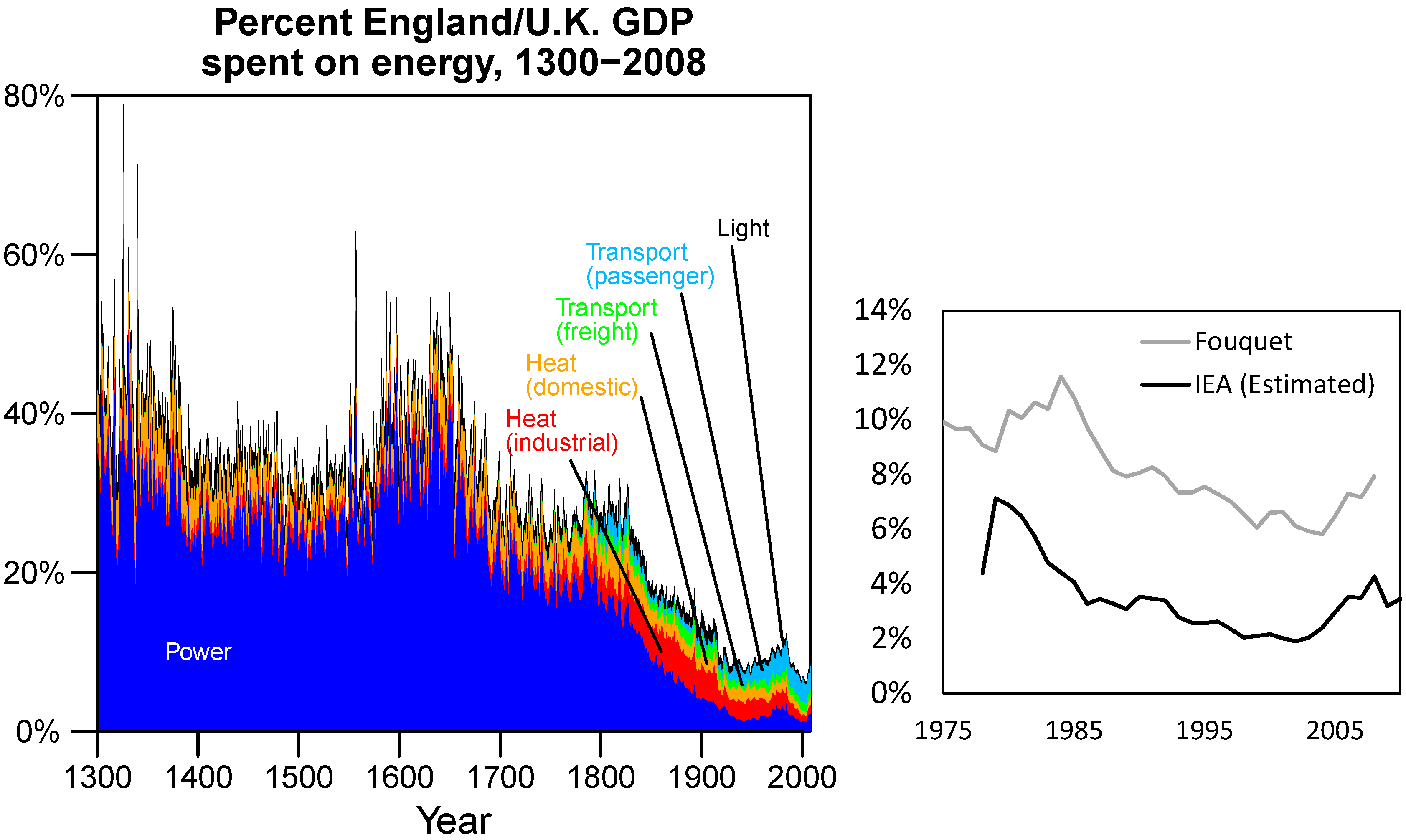
2.2. England and United Kingdom Data
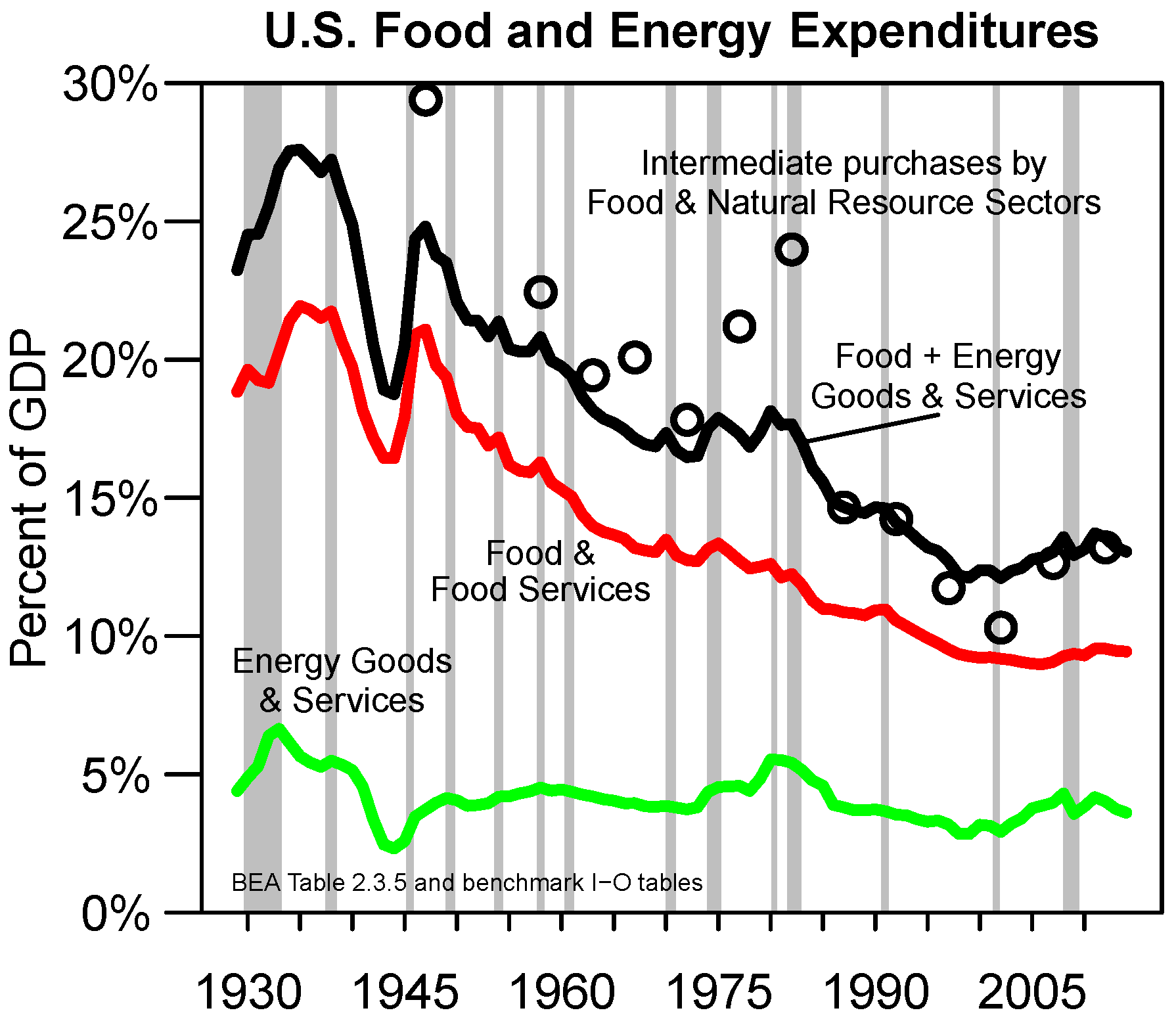
2.3. United States Data
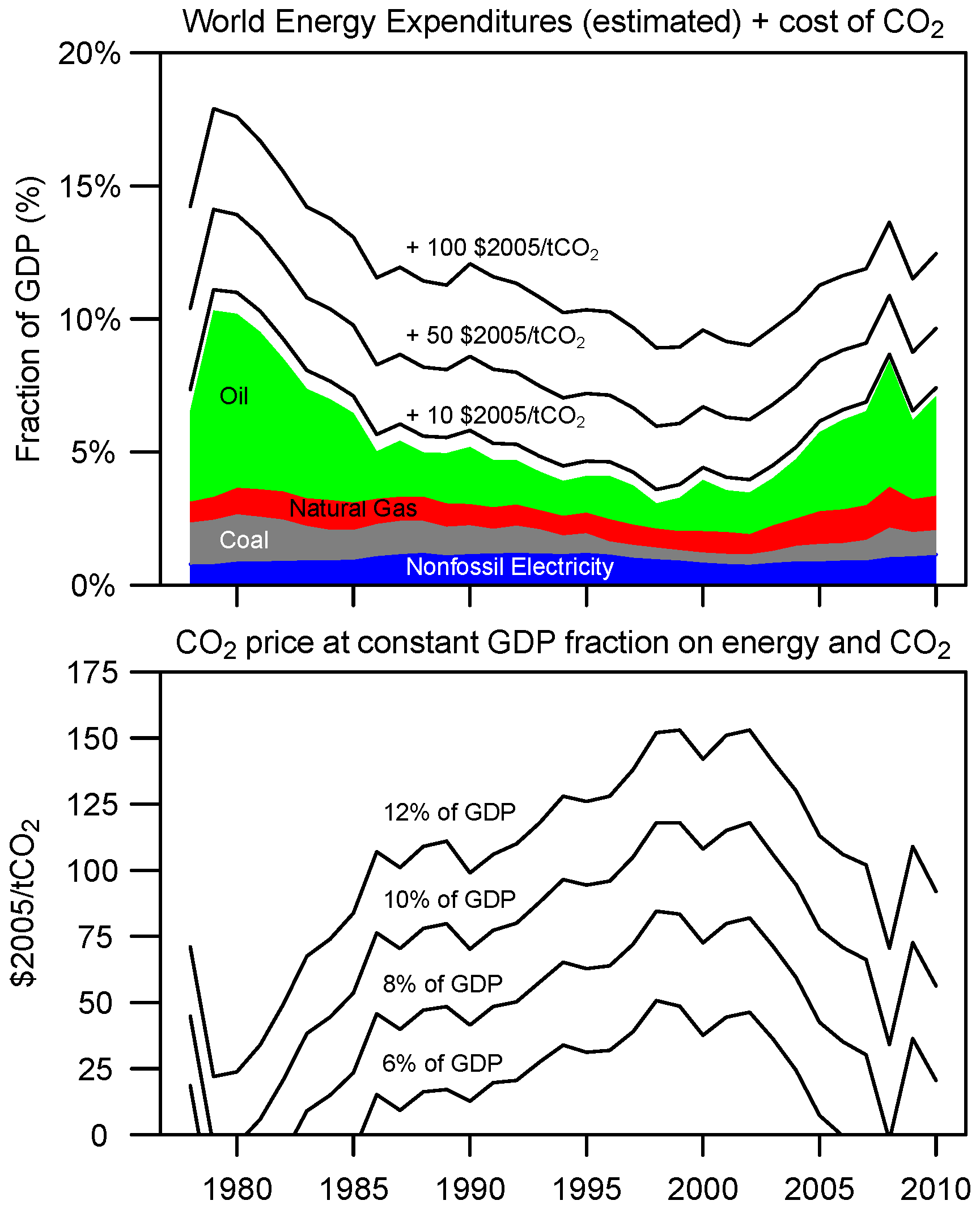
2.4. Emissions from Energy Consumption
3. Results
- Global expenditures on energy expressed as a fraction of GDP is significantly correlated with the one-year lag of the annual changes in both GDP and total factor productivity, but not with zero-year lag.
- The one-year lag correlation is statistically significant only when including expenditures for oil and when considering oil expenditures only.
3.1. Correlation of to GDP and Total Factor Productivity
- for 1-year lagged ΔGDP: United Kingdom, Spain, The Netherlands, Sweden, Greece, Nigeria, and Portugal (see Table 1).
- for 1-year lagged ΔTFP from TED: United States, Russia, Canada, France, Sweden, and Greece (see Table 2).
- for 1-year lagged ΔMFP from OECD: The Netherlands, Canada, France, Sweden, and South Korea (see Table 2).

| Country | % of GDP on Energy (Actual Data) | % of GDP on Energy (Estimated) | ||
|---|---|---|---|---|
| Correlation Coefficient | p Value | Correlation Coefficient | p Value | |
| USA | −0.263 | 0.145 | −0.284 | 0.115 |
| UK | −0.289 | 0.109 | −0.451 | 0.010 ** |
| SPAIN | −0.463 | 0.008 ** | −0.623 | 0.0001 ** |
| RUSSIA | 0.121 | 0.508 | −0.0397 | 0.829 |
| NETHERLANDS | −0.494 | 0.004 ** | −0.452 | 0.010 ** |
| JAPAN | 0.073 | 0.69 | 0.14 | 0.443 |
| ITALY | −0.472 | 0.006 * | −0.327 | 0.068 |
| GERMANY | 0.12 | 0.513 | 0.102 | 0.578 |
| CANADA | −0.359 | 0.044 * | −0.319 | 0.075 |
| FRANCE | −0.514 | 0.003 ** | −0.323 | 0.071 |
| AUSTRIA | −0.35 | 0.049 * | −0.337 | 0.060 |
| DENMARK | −0.273 | 0.13 | −0.303 | 0.092 |
| FINLAND | −0.129 | 0.481 | −0.0398 | 0.829 |
| NORWAY | −0.382 | 0.031 * | 0.127 | 0.487 |
| SWEDEN | −0.469 | 0.007 ** | −0.362 | 0.042 * |
| ARGENTINA | 0.411 | 0.019 * | 0.09 | 0.624 |
| AUSTRALIA | −0.185 | 0.311 | −0.237 | 0.192 |
| BELGIUM | −0.587 | 0.0004 ** | −0.328 | 0.066 |
| BRAZIL | −0.133 | 0.468 | −0.038 | 0.838 |
| CHINA | 0.359 | 0.044 * | −0.129 | 0.481 |
| TAIPEI | −0.515 | 0.003 ** | 0.104 | 0.57 |
| COLOMBIA | 0.063 | 0.732 | −0.019 | 0.918 |
| CZECH | 0.167 | 0.361 | 0.058 | 0.751 |
| GREECE | −0.439 | 0.012 * | −0.452 | 0.010 ** |
| HUNGARY | −0.389 | 0.028 * | −0.194 | 0.287 |
| INDIA | 0.46 | 0.008 ** | 0.138 | 0.452 |
| INDONESIA | −0.089 | 0.628 | 0.097 | 0.598 |
| IRAN | 0.246 | 0.175 | −0.010 | 0.956 |
| IRAQ | 0.347 | 0.052 | 0.265 | 0.142 |
| S KOREA | −0.434 | 0.013 * | −0.291 | 0.107 |
| KUWAIT | −0.197 | 0.279 | −0.293 | 0.104 |
| LIBYA | 0.112 | 0.541 | 0.179 | 0.328 |
| MALAYSIA | −0.24 | 0.186 | −0.215 | 0.238 |
| MEXICO | −0.184 | 0.314 | −0.195 | 0.285 |
| NEW ZEALAND | −0.082 | 0.655 | −0.206 | 0.258 |
| NIGERIA | 0.143 | 0.436 | −0.377 | 0.033 * |
| POLAND | 0.085 | 0.645 | −0.302 | 0.093 |
| PORTUGAL | −0.497 | 0.004 ** | −0.394 | 0.026 * |
| QATAR | 0.478 | 0.006 ** | 0.373 | 0.036 * |
| SAUDI ARABIA | −0.101 | 0.581 | −0.133 | 0.467 |
| S AFRICA | 0.087 | 0.635 | −0.017 | 0.926 |
| SWITZERLAND | −0.090 | 0.625 | −0.032 | 0.864 |
| TURKEY | −0.035 | 0.85 | −0.215 | 0.237 |
| VENEZUELA | 0.252 | 0.164 | −0.083 | 0.65 |
| WORLD | −0.369 | 0.038 * | −0.447 | 0.010 * |
| Country | TED TFP | OECD MFP | ||||||
|---|---|---|---|---|---|---|---|---|
| Actual | Estimated | Actual | Estimated | |||||
| Correlation Coefficient | p Value | Correlation Coefficient | p Value | Correlation Coefficient | p Value | Correlation Coefficient | p Value | |
| USA | −0.565 | 0.009 ** | −0.545 | 0.011 * | −0.306 | 0.137 | −0.306 | 0.137 |
| UK | −0.456 | 0.043 * | −0.416 | 0.068 | −0.432 | 0.035 * | -0.389 | 0.060 |
| SPAIN | −0.315 | 0.176 | -0.317 | 0.173 | −0.047 | 0.825 | −0.065 | 0.757 |
| RUSSIA | −0.269 | 0.296 | −0.521 | 0.032 * | – | – | – | – |
| NETHERLANDS | −0.420 | 0.065 | −0.314 | 0.178 | −0.431 | 0.031 * | −0.435 | 0.030 * |
| JAPAN | −0.317 | 0.173 | −0.104 | 0.663 | −0.215 | 0.301 | −0.207 | 0.321 |
| ITALY | −0.216 | 0.361 | −0.314 | 0.178 | −0.249 | 0.230 | −0.360 | 0.077 |
| GERMANY | −0.075 | 0.753 | −0.107 | 0.654 | −0.245 | 0.327 | −0.273 | 0.272 |
| CANADA | −0.650 | 0.002 ** | −0.642 | 0.002 ** | −0.464 | 0.019 * | −0.491 | 0.013* |
| FRANCE | −0.616 | 0.004 ** | −0.635 | 0.003 ** | −0.577 | 0.003 ** | −0.461 | 0.020 * |
| AUSTRIA | −0.155 | 0.514 | −0.159 | 0.504 | −0.191 | 0.512 | −0.237 | 0.415 |
| DENMARK | −0.109 | 0.648 | −0.391 | 0.088 | −0.070 | 0.740 | −0.369 | 0.069 |
| FINLAND | −0.341 | 0.142 | −0.290 | 0.215 | −0.355 | 0.082 | −0.301 | 0.144 |
| NORWAY | −0.299 | 0.200 | 0.060 | 0.800 | – | – | – | – |
| SWEDEN | −0.456 | 0.043 * | −0.490 | 0.028 * | −0.491 | 0.013 * | −0.418 | 0.037* |
| ARGENTINA | 0.049 | 0.837 | 0.008 | 0.974 | – | – | – | – |
| AUSTRALIA | 0.083 | 0.727 | −0.324 | 0.163 | −0.059 | 0.790 | −0.287 | 0.184 |
| BELGIUM | −0.411 | 0.072 | −0.352 | 0.128 | −0.423 | 0.035 * | -0.330 | 0.107 |
| BRAZIL | 0.068 | 0.775 | −0.239 | 0.311 | – | – | – | – |
| CHINA | −0.063 | 0.793 | 0.048 | 0.842 | – | – | – | – |
| TAIPEI | – | – | – | – | – | – | – | – |
| COLOMBIA | 0.015 | 0.952 | -0.039 | 0.872 | – | – | – | – |
| CZECH | −0.078 | 0.766 | 0.002 | 0.995 | – | – | – | – |
| GREECE | −0.431 | 0.058 | −0.451 | 0.046* | – | – | – | – |
| HUNGARY | −0.404 | 0.077 | −0.416 | 0.068 | – | – | – | – |
| INDIA | 0.115 | 0.630 | 0.002 | 0.994 | – | – | – | – |
| INDONESIA | 0.177 | 0.455 | 0.102 | 0.669 | – | – | – | – |
| IRAN | 0.055 | 0.818 | 0.054 | 0.822 | – | – | – | – |
| IRAQ | 0.306 | 0.190 | 0.232 | 0.325 | – | – | – | – |
| S KOREA | −0.102 | 0.670 | −0.301 | 0.197 | −0.409 | 0.042 * | −0.480 | 0.015* |
| KUWAIT | −0.135 | 0.572 | -0.118 | 0.620 | – | – | – | – |
| LIBYA | – | – | – | – | – | – | – | – |
| MALAYSIA | −0.105 | 0.658 | −0.072 | 0.762 | – | – | – | – |
| MEXICO | −0.348 | 0.133 | −0.349 | 0.132 | – | – | – | – |
| NEW ZEALAND | -0.431 | 0.058 | −0.417 | 0.067 | -0.169 | 0.420 | -0.144 | 0.493 |
| NIGERIA | −0.159 | 0.504 | −0.024 | 0.920 | – | – | – | – |
| POLAND | −0.277 | 0.237 | 0.245 | 0.297 | – | – | – | – |
| PORTUGAL | −0.024 | 0.920 | −0.046 | 0.846 | −0.236 | 0.397 | −0.262 | 0.345 |
| QATAR | −0.039 | 0.869 | 0.030 | 0.901 | – | – | – | – |
| SAUDI ARABIA | −0.290 | 0.215 | −0.268 | 0.254 | – | – | – | – |
| S AFRICA | −0.145 | 0.542 | −0.297 | 0.204 | – | – | – | – |
| SWITZERLAND | −0.162 | 0.496 | −0.147 | 0.536 | −0.076 | 0.757 | −0.056 | 0.819 |
| TURKEY | −0.192 | 0.417 | −0.214 | 0.365 | – | – | – | – |
| VENEZUELA | 0.051 | 0.831 | −0.017 | 0.942 | – | – | – | – |
| WORLD | −0.531 | 0.016 * | −0.490 | 0.028 * | −0.520 | 0.008 ** | −0.509 | 0.009 ** |
| Country | % of GDP on Oil (Actual Data, 1-Year Lag) | % of GDP on Oil (Estimated, 1-Year Lag) | ||
|---|---|---|---|---|
| Correlation Coefficient | p Value | Correlation Coefficient | p Value | |
| USA | −0.296 | 0.112 | −0.364 | 0.041 * |
| UK | −0.314 | 0.0905 | −0.451 | 0.010 ** |
| SPAIN | −0.572 | 0.001 ** | −0.524 | 0.002 ** |
| RUSSIA | −0.050 | 0.794 | 0.055 | 0.766 |
| NETHERLANDS | −0.533 | 0.002 ** | −0.39 | 0.027 * |
| JAPAN | 0.121 | 0.523 | 0.145 | 0.427 |
| ITALY | −0.189 | 0.316 | −0.045 | 0.806 |
| GERMANY | −0.196 | 0.3 | −0.169 | 0.354 |
| CANADA | −0.322 | 0.0829 | −0.272 | 0.132 |
| FRANCE | −0.476 | 0.008 ** | −0.234 | 0.198 |
| AUSTRIA | −0.461 | 0.010 * | −0.376 | 0.034 * |
| DENMARK | −0.106 | 0.577 | −0.112 | 0.543 |
| FINLAND | −0.141 | 0.459 | 0.007 | 0.971 |
| NORWAY | −0.196 | 0.3 | −0.035 | 0.849 |
| SWEDEN | −0.228 | 0.225 | −0.189 | 0.301 |
| ARGENTINA | 0.445 | 0.014 * | −0.092 | 0.616 |
| AUSTRALIA | −0.263 | 0.161 | −0.224 | 0.218 |
| BELGIUM | −0.565 | 0.001 ** | −0.311 | 0.084 |
| BRAZIL | 0.174 | 0.358 | 0.024 | 0.898 |
| CHINA | 0.282 | 0.132 | −0.163 | 0.371 |
| TAIPEI | −0.495 | 0.005 ** | 0.15 | 0.412 |
| COLOMBIA | −0.003 | 0.987 | −0.104 | 0.57 |
| CZECH | 0.238 | 0.206 | −0.119 | 0.517 |
| GREECE | −0.434 | 0.017 * | −0.432 | 0.014 * |
| HUNGARY | −0.298 | 0.109 | −0.105 | 0.566 |
| INDIA | 0.383 | 0.037 * | 0.145 | 0.43 |
| INDONESIA | −0.052 | 0.787 | 0.113 | 0.539 |
| IRAN | 0.118 | 0.534 | −0.083 | 0.652 |
| IRAQ | 0.398 | 0.029 * | 0.268 | 0.138 |
| S KOREA | −0.66 | 7.0× ** | −0.183 | 0.317 |
| KUWAIT | −0.178 | 0.347 | −0.29 | 0.107 |
| LIBYA | 0.056 | 0.769 | 0.163 | 0.371 |
| MALAYSIA | −0.255 | 0.173 | −0.223 | 0.22 |
| MEXICO | −0.065 | 0.734 | −0.145 | 0.427 |
| NEW ZEALAND | −0.090 | 0.637 | −0.133 | 0.468 |
| NIGERIA | 0.219 | 0.246 | −0.413 | 0.019 * |
| POLAND | −0.034 | 0.86 | −0.257 | 0.156 |
| PORTUGAL | −0.456 | 0.011 * | −0.362 | 0.042 * |
| QATAR | 0.36 | 0.051 | 0.412 | 0.019 * |
| SAUDI ARABIA | −0.235 | 0.21 | −0.158 | 0.388 |
| S AFRICA | 0.106 | 0.576 | 0.031 | 0.865 |
| SWITZERLAND | −0.118 | 0.533 | 0.009 | 0.961 |
| TURKEY | −0.103 | 0.589 | −0.161 | 0.378 |
| VENEZUELA | 0.172 | 0.363 | −0.163 | 0.373 |
| WORLD | −0.469 | 0.009 ** | −0.364 | 0.040 * |
| Country | TED TFP | OECD MFP | ||||||
|---|---|---|---|---|---|---|---|---|
| Actual | Estimated | Actual | Estimated | |||||
| Correlation Coefficient | p Value | Correlation Coefficient | p Value | Correlation Coefficient | p Value | Correlation Coefficient | p Value | |
| USA | −0.547 | 0.013 * | −0.547 | 0.013 * | −0.245 | 0.239 | −0.245 | 0.239 |
| UK | −0.546 | 0.013 * | −0.546 | 0.013 * | −0.416 | 0.043 * | −0.416 | 0.043 * |
| SPAIN | −0.432 | 0.057 | −0.432 | 0.057 | −0.217 | 0.296 | −0.217 | 0.296 |
| RUSSIA | −0.508 | 0.038 * | −0.489 | 0.046 * | – | – | – | – |
| NETHERLANDS | −0.340 | 0.143 | −0.340 | 0.143 | −0.382 | 0.059 | −0.382 | 0.059 |
| JAPAN | −0.205 | 0.385 | −0.205 | 0.385 | −0.296 | 0.151 | −0.296 | 0.151 |
| ITALY | −0.464 | 0.039 * | −0.464 | 0.039 * | −0.355 | 0.082 | −0.355 | 0.082 |
| GERMANY | −0.426 | 0.061 | −0.426 | 0.061 | −0.423 | 0.081 | −0.423 | 0.081 |
| CANADA | −0.682 | 0.001 ** | −0.682 | 0.001 ** | −0.554 | 0.004 ** | −0.554 | 0.004 ** |
| FRANCE | −0.552 | 0.012 * | −0.656 | 0.002 ** | −0.575 | 0.003 ** | −0.512 | 0.009 ** |
| AUSTRIA | −0.221 | 0.350 | −0.221 | 0.350 | −0.306 | 0.288 | −0.306 | 0.288 |
| DENMARK | −0.505 | 0.023 * | −0.505 | 0.023 * | −0.386 | 0.057 | −0.386 | 0.057 |
| FINLAND | −0.381 | 0.097 | −0.623 | 0.003 ** | −0.394 | 0.052 | −0.469 | 0.018 * |
| NORWAY | −0.696 | 0.001 ** | −0.696 | 0.001 ** | – | – | – | – |
| SWEDEN | −0.592 | 0.006 ** | −0.592 | 0.006 ** | −0.364 | 0.074 | −0.364 | 0.074 |
| ARGENTINA | −0.005 | 0.983 | −0.005 | 0.982 | – | – | – | – |
| AUSTRALIA | −0.423 | 0.063 | −0.423 | 0.063 | −0.347 | 0.105 | −0.347 | 0.105 |
| BELGIUM | −0.409 | 0.073 | −0.409 | 0.073 | −0.427 | 0.033 * | −0.427 | 0.033 * |
| BRAZIL | −0.316 | 0.175 | −0.316 | 0.175 | – | – | – | – |
| CHINA | 0.154 | 0.517 | 0.153 | 0.519 | – | – | – | – |
| TAIPEI | – | – | – | – | – | – | – | – |
| COLOMBIA | −0.118 | 0.621 | −0.118 | 0.620 | – | – | – | – |
| CZECH | 0.095 | 0.716 | −0.114 | 0.663 | – | – | – | – |
| GREECE | −0.388 | 0.091 | −0.388 | 0.091 | – | – | – | – |
| HUNGARY | −0.434 | 0.056 | −0.435 | 0.055 | – | – | – | – |
| INDIA | 0.097 | 0.684 | 0.076 | 0.751 | – | – | – | – |
| INDONESIA | 0.094 | 0.694 | 0.097 | 0.683 | – | – | – | – |
| IRAN | 0.056 | 0.813 | 0.058 | 0.809 | – | – | – | – |
| IRAQ | 0.281 | 0.230 | 0.236 | 0.317 | – | – | – | – |
| S KOREA | −0.147 | 0.537 | −0.275 | 0.241 | −0.513 | 0.009 ** | −0.402 | 0.046 * |
| KUWAIT | −0.185 | 0.436 | −0.104 | 0.662 | – | – | – | – |
| LIBYA | – | – | – | – | – | – | – | – |
| MALAYSIA | −0.115 | 0.628 | −0.101 | 0.671 | – | – | – | – |
| MEXICO | −0.340 | 0.142 | −0.340 | 0.142 | – | – | – | – |
| NEW ZEALAND | −0.331 | 0.154 | −0.331 | 0.154 | −0.120 | 0.566 | −0.120 | 0.566 |
| NIGERIA | 0.071 | 0.768 | 0.072 | 0.764 | – | – | – | – |
| POLAND | −0.280 | 0.233 | −0.429 | 0.059 | – | – | – | – |
| PORTUGAL | −0.204 | 0.388 | −0.204 | 0.388 | −0.364 | 0.182 | −0.364 | 0.182 |
| QATAR | −0.037 | 0.879 | −0.144 | 0.546 | – | – | – | – |
| SAUDI ARABIA | −0.352 | 0.128 | −0.288 | 0.219 | – | – | – | – |
| S AFRICA | −0.229 | 0.331 | −0.229 | 0.331 | – | – | – | – |
| SWITZERLAND | −0.164 | 0.488 | −0.164 | 0.488 | −0.132 | 0.591 | −0.132 | 0.591 |
| TURKEY | −0.290 | 0.215 | −0.290 | 0.215 | – | – | – | – |
| VENEZUELA | −0.067 | 0.780 | −0.067 | 0.779 | – | – | – | – |
| WORLD | −0.479 | 0.033 * | −0.483 | 0.031 * | −0.542 | 0.005 ** | −0.524 | 0.007 ** |
| Country | TED TFP | OECD MFP | ||||||
|---|---|---|---|---|---|---|---|---|
| Actual | Estimated | Actual | Estimated | |||||
| Correlation Coefficient | p Value | Correlation Coefficient | p Value | Correlation Coefficient | p Value | Correlation Coefficient | p Value | |
| USA | −0.481 | 0.032 * | −0.478 | 0.033 * | −0.366 | 0.072 | −0.366 | 0.072 |
| UK | −0.295 | 0.206 | −0.205 | 0.385 | −0.337 | 0.107 | −0.258 | 0.223 |
| SPAIN | 0.035 | 0.884 | −0.037 | 0.877 | 0.334 | 0.103 | 0.231 | 0.267 |
| RUSSIA | −0.177 | 0.497 | −0.465 | 0.060 | – | – | – | – |
| NETHERLANDS | −0.377 | 0.101 | −0.153 | 0.520 | −0.334 | 0.103 | −0.345 | 0.092 |
| JAPAN | −0.091 | 0.704 | 0.183 | 0.440 | 0.126 | 0.550 | 0.186 | 0.373 |
| ITALY | −0.076 | 0.749 | −0.204 | 0.389 | −0.157 | 0.455 | −0.310 | 0.131 |
| GERMANY | 0.053 | 0.826 | 0.017 | 0.943 | −0.114 | 0.653 | −0.157 | 0.533 |
| CANADA | −0.498 | 0.025 * | −0.403 | 0.078 | −0.241 | 0.247 | −0.243 | 0.242 |
| FRANCE | −0.456 | 0.043 * | −0.397 | 0.083 | −0.298 | 0.148 | −0.221 | 0.289 |
| AUSTRIA | −0.018 | 0.940 | −0.066 | 0.781 | −0.015 | 0.959 | −0.145 | 0.621 |
| DENMARK | 0.422 | 0.064 | −0.253 | 0.282 | 0.381 | 0.060 | −0.263 | 0.204 |
| FINLAND | −0.160 | 0.501 | 0.240 | 0.307 | −0.213 | 0.306 | 0.100 | 0.636 |
| NORWAY | −0.112 | 0.638 | 0.376 | 0.102 | – | – | – | – |
| SWEDEN | −0.379 | 0.100 | −0.322 | 0.166 | −0.451 | 0.024 * | −0.286 | 0.166 |
| ARGENTINA | 0.283 | 0.227 | 0.023 | 0.925 | – | – | – | – |
| AUSTRALIA | 0.597 | 0.005 ** | −0.043 | 0.859 | 0.250 | 0.250 | −0.039 | 0.860 |
| BELGIUM | −0.292 | 0.211 | −0.149 | 0.532 | −0.179 | 0.391 | −0.020 | 0.923 |
| BRAZIL | 0.251 | 0.286 | 0.017 | 0.942 | – | – | – | – |
| CHINA | −0.143 | 0.548 | −0.010 | 0.967 | – | – | – | – |
| TAIPEI | – | – | – | – | – | – | – | – |
| COLOMBIA | 0.337 | 0.146 | 0.142 | 0.551 | – | – | – | – |
| CZECH | −0.330 | 0.196 | 0.055 | 0.835 | – | – | – | – |
| GREECE | −0.606 | 0.005 ** | −0.595 | 0.006 ** | – | – | – | – |
| HUNGARY | −0.159 | 0.504 | −0.381 | 0.097 | – | – | – | – |
| INDIA | 0.132 | 0.580 | −0.165 | 0.487 | – | – | – | – |
| INDONESIA | 0.036 | 0.880 | 0.107 | 0.653 | – | – | – | – |
| IRAN | −0.030 | 0.901 | 0.045 | 0.850 | – | – | – | – |
| IRAQ | 0.092 | 0.700 | 0.077 | 0.747 | – | – | – | – |
| S KOREA | 0.046 | 0.846 | −0.254 | 0.279 | 0.115 | 0.583 | −0.441 | 0.028 * |
| KUWAIT | 0.052 | 0.829 | −0.338 | 0.145 | – | – | – | – |
| LIBYA | – | – | – | – | – | – | – | – |
| MALAYSIA | 0.116 | 0.627 | 0.051 | 0.832 | – | – | – | – |
| MEXICO | −0.335 | 0.149 | −0.350 | 0.130 | – | – | – | – |
| NEW ZEALAND | −0.424 | 0.063 | −0.381 | 0.097 | −0.158 | 0.451 | −0.109 | 0.604 |
| NIGERIA | −0.177 | 0.455 | −0.569 | 0.009 ** | – | – | – | – |
| POLAND | −0.021 | 0.930 | 0.476 | 0.034 * | – | – | – | – |
| PORTUGAL | 0.196 | 0.408 | 0.212 | 0.370 | −0.044 | 0.878 | −0.064 | 0.821 |
| QATAR | 0.000 | 0.999 | 0.271 | 0.248 | – | – | – | – |
| SAUDI ARABIA | 0.319 | 0.170 | −0.037 | 0.876 | – | – | – | – |
| S AFRICA | 0.177 | 0.455 | −0.383 | 0.096 | – | – | – | – |
| SWITZERLAND | −0.013 | 0.956 | 0.004 | 0.987 | 0.044 | 0.859 | 0.075 | 0.760 |
| TURKEY | −0.125 | 0.598 | −0.138 | 0.561 | – | – | – | – |
| VENEZUELA | 0.307 | 0.188 | 0.245 | 0.297 | – | – | – | – |
| WORLD | −0.372 | 0.106 | −0.412 | 0.071 | −0.261 | 0.207 | −0.310 | 0.132 |
3.2. England and the United Kingdom

3.3. The United States

4. Discussion
4.1. Historical Context of Expenditures on Energy
4.2. Relevance for Internalizing Emissions

4.2.1. The Energy Trap
4.2.2. Internalizing Emissions into
4.2.3. Summary of Relevance for Internalizing Emissions
4.3. Broader Considerations for Policy and Future Research
5. Conclusions
Supplementary Files
Supplementary File 1Supplementary File 2Acknowledgments
Conflicts of Interest
References
- King, C.W.; Maxwell, J.P.; Donovan, A. Comparing world economic and net energy metrics, Part 1: Price Perspective. Energies 2015, 8, 12949–12974. [Google Scholar] [CrossRef]
- King, C.W.; Maxwell, J.P.; Donovan, A. Comparing world economic and net energy metrics, Part 2: Expenditures Perspective. Energies 2015, 8, 12975–12996. [Google Scholar] [CrossRef]
- Solow, R. A Contribution to the Theory of Economic-Growth. Q. J. Econ. 1956, 70, 65–94. [Google Scholar] [CrossRef]
- Hamilton, J. Historical Oil Shocks. In Routledge Handbook of Major Events in Economic History; Parker, R.E., Whaples, R.M., Eds.; Routledge: New York, NY, USA, 2013; p. 239265. [Google Scholar]
- Ayres, R.; Voudouris, V. The economic growth enigma: Capital, labour and useful energy? Energy Policy 2014, 64, 16–28. [Google Scholar] [CrossRef]
- Voudouris, V.; Ayres, R.; Serrenho, A.C.; Kiose, D. The economic growth enigma revisited: The EU-15 since the 1970s. Energy Policy 2015. [Google Scholar] [CrossRef]
- Kander, A.; Stern, D.I. Economic growth and the transition from traditional to modern energy in Sweden. Energy Econ. 2014, 46, 56–65. [Google Scholar] [CrossRef]
- Kümmel, R. The Second Law of Economics: Energy, Entropy, and the Origins of Wealth; Springer: Berlin, Germany, 2011. [Google Scholar]
- Hall, C.A.S.; Klitgaard, K.A. Energy and the Wealth of Nations: Understanding the Biophysical Economy, 1st ed.; Springer: Berlin, Germany, 2012. [Google Scholar]
- Ayres, R.U. Sustainability economics: Where do we stand? Ecol. Econ. 2008, 67, 281–310. [Google Scholar] [CrossRef]
- Brown, J.H.; Burnside, W.R.; Davidson, A.D.; Delong, J.R.; Dunn, W.C.; Hamilton, M.J.; Mercado-Silva, N.; Nekola, J.C.; Okie, J.G.; Woodruff, W.H.; et al. Energetic Limits to Economic Growth. BioScience 2011, 61, 19–26. [Google Scholar] [CrossRef]
- Peters, G.P.; Hertwich, E.G. CO2 embodied in international trade with implications for global climate policy. Environ. Sci. Technol. 2008, 42, 1401–1407. [Google Scholar] [CrossRef] [PubMed]
- Acemoglu, D.; Robinson, J.A. Why Nations Fail: The Origins of Power, Prosperity, and Poverty; Crown Business: New York, NY, USA, 2012. [Google Scholar]
- Tainter, J. The Collapse of Complex Societies; Cambridge University Press: Cambridge, UK, 1988. [Google Scholar]
- Tainter, J.A. Energy, complexity, and sustainability: A historical perspective. Environ. Innov. Soc. Transit. 2011, 1, 89–95. [Google Scholar] [CrossRef]
- Tainter, J.A. Energy and Existential Sustainability: The Role of Reserve Capacity. J. Environ. Account. Manag. 2013, 1, 213–228. [Google Scholar] [CrossRef]
- Turchin, P.; Nefedov, S.A. Secular Cycles; Princeston University Press: Princeston, NJ, USA, 2009. [Google Scholar]
- Ayres, R.U.; Warr, B. Accounting for growth: The role of physical work. Struct. Chang. Econ. Dyn. 2005, 16, 181–209. [Google Scholar] [CrossRef]
- Stern, D.; Kander, A. The Role of Energy in the Industrial Revolution and Modern Economic Growth; Technical Report; The Australian National University: Canberra, Australia, 2011. [Google Scholar]
- Stern, D.I.; Kander, A. The Role of Energy in the Industrial Revolution and Modern Economic Growth. Energy J. 2012, 33. [Google Scholar] [CrossRef]
- Hamilton, J. Causes and Consequences of the Oil Shock of 2007–08. In Brookings Papers on Economic Activity; Romer, D., Wolfers, J., Eds.; Brookings Institution Press: Washington, DC, USA, 2009; p. 69. [Google Scholar]
- Hall, C.A.S.; Cleveland, C.J.; Kaufmann, R.K. Energy and Resource Quality: ThE Ecology of the Economic Process; Wiley: New York, NY, USA, 1986. [Google Scholar]
- Hall, C.A.S.; Balogh, S.; Murphy, D.J.R. What is the Minimum EROI that a Sustainable Society Must Have? Energies 2009, 2, 25–47. [Google Scholar] [CrossRef]
- King, C.W. Energy intensity ratios as net energy measures of United States energy production and expenditures. Environ. Res. Lett. 2010, 5, 044006. [Google Scholar] [CrossRef]
- Brandt, A.R. Converting oil shale to liquid fuels: Energy inputs and greenhouse gas emissions of the Shell in situ conversion process. Environ. Sci. Technol. 2008, 42, 7489–7495. [Google Scholar] [CrossRef] [PubMed]
- Brandt, A.R. Converting Oil Shale to Liquid Fuels with the Alberta Taciuk Processor: Energy Inputs and Greenhouse Gas Emissions. EnergyFuels 2009, 23, 6253–6258. [Google Scholar] [CrossRef]
- Brandt, A.R.; Englander, J.; Bharadwaj, S. The energy efficiency of oil sands extraction: Energy return ratios from 1970 to 2010. Energy 2013, 55, 693–702. [Google Scholar] [CrossRef]
- Guilford, M.C.; Hall, C.A.S.; O’Connor, P.; Cleveland, C.J. A New Long Term Assessment of Energy Return on Investment (EROI) for US Oil and Gas Discovery and Production. Sustainability 2011, 3, 1866–1887. [Google Scholar] [CrossRef]
- Farrell, A.E.; Plevin, R.J.; Turner, B.T.; Jones, A.D.; O’Hare, M.; Kammen, D.M. Ethanol can contribute to energy and environmental goals. Science 2006, 311, 506–508. [Google Scholar] [CrossRef] [PubMed]
- Raugei, M.; Fullana-i-Palmer, P.; Fthenakis, V. The energy return on energy investment (EROI) of photovoltaics: Methodology and comparisons with fossil fuel life cycles. Energy Policy 2012, 45, 576–582. [Google Scholar] [CrossRef]
- Dale, M.; Benson, S.M. Energy Balance of the Global Photovoltaic (PV) Industry—Is the PV Industry a Net Electricity Producer? Environ. Sci. Technol. 2013, 47, 3482–3489. Available online: http://pubs.acs.org/doi/pdf/10.1021/es3038824 (accessed on 3 March 2015). [Google Scholar] [CrossRef] [PubMed]
- Fthenakis, V.M.; Kim, H.C. Photovoltaics: Life-cycle analyses. Sol. Energy 2011, 85, 1609–1628. [Google Scholar] [CrossRef]
- Zhang, Y.; Colosi, L.M. Practical ambiguities during calculation of energy ratios and their impacts on life cycle assessment calculations. Energy Policy 2013, 57, 630–633. [Google Scholar] [CrossRef]
- Bullard, C.W., III; Herendeen, R.A. The energy cost of goods and services. Energy Policy 1975, 3, 268–278. [Google Scholar] [CrossRef]
- Costanza, R. Embodied Energy and Economic Valuation. Science 1980, 210, 1219–1224. [Google Scholar] [CrossRef] [PubMed]
- King, C.W.; Hall, C.A.S. Relating Financial and Energy Return on Investment. Sustainability 2011, 3, 1810–1832. [Google Scholar] [CrossRef]
- Henshaw, P.F.; King, C.; Zarnikau, J. System Energy Assessment (SEA), Defining a Standard Measure of EROI for Energy Businesses as Whole Systems. Sustainability 2011, 3, 1908–1943. [Google Scholar] [CrossRef]
- Summers, L.H. Have We Entered an Age of Secular Stagnation? IMF Econ. Rev. 2015, 63, 277–280. [Google Scholar] [CrossRef]
- Gordon, R.J. Is US Economic Growth Over? Faltering Innovation Confronts the Six Headwinds; NBER Working Paper No. 18315; National Bureau of Economic Research (NBER): Cambridge, MA, USA, 2012. [Google Scholar]
- Meadows, D.H.; Meadows, D.L.; Randers, J.; Behrens, W.W.I. Limits to Growth: A Report for the Club of Rome’s Project on the Predicament of Mankind; Universe Books: New York, NY, USA, 1972. [Google Scholar]
- Meadows, D.H.; Randers, J.; Meadows, D.L. Limits to Growth: The 30-Year Update; Chelsea Green Publishing: White River Junction, VT, USA, 2004. [Google Scholar]
- Kilian, L. Oil Price Shocks, Monetary Policy and Stagflation. In Proceedings of Conference on Inflation in an Era of Relative Price Shocks, Sydney, Australia, 17–18 August 2009; Available online: http://www-personal.umich.edu/ lkilian/rbakilianpub.pdf (accessed on 3 March 2015).
- Kopits, S. Oil: What Price can America afford? Available online: http://www.oilandgasinvestor.com/oil-what-price-can-america-afford-465256 (accessed on 3 March 2015).
- Bashmakov, I. Three laws of energy transitions. Energy Policy 2007, 35, 3583–3594. [Google Scholar] [CrossRef]
- Kalimeris, P.; Richardson, C.; Bithas, K. A meta-analysis investigation of the direction of the energy—GDP causal relationship: implications for the growth-degrowth dialogue. J. Clean. Prod. 2014, 67, 1–13. [Google Scholar] [CrossRef]
- Cleveland, C.J.; Kaufmann, R.K.; Stern, D.I. Aggregation and the role of energy in the economy. Ecol. Econ. 2000, 32, 301–317. [Google Scholar] [CrossRef]
- Odum, H.T. Environmental Accounting: Energy and Environmental Decision Making; John Wiley & Sons, Inc.: New York, NY, USA, 1996. [Google Scholar]
- Campbell, D.E.; Lu, H.; Walker, H.A. Relationships among the Energy, Emergy and Money Flows of the United States from 1900 to 2011. Front. Energy Res. 2014, 2. [Google Scholar] [CrossRef]
- Stern, D.I. Energy and economic growth in the USA: A multivariate approach. Energy Econ. 1993, 15, 137–150. [Google Scholar] [CrossRef]
- Cleveland, C.J.; Costanza, R.; Hall, C.A.S.; Kaufmann, R.K. Energy and the US Economy: A Biophysical Perspective. Science 1984, 225, 890–897. [Google Scholar] [CrossRef] [PubMed]
- Stern, D.I. The role of energy in economic growth. Ann. N. Y. Acad. Sci. 2011, 1219, 26–51. [Google Scholar] [CrossRef] [PubMed]
- The Conference Board. Total Economy Database, 2013. Available online: http://www.conference-board.org/data/economydatabase (accessed 17 December 2013).
- Organization for Economic Co-operation and Development. OECD. Stat Database, 2013. Available online: http://stats.oecd.org (accessed 17 December 2013).
- Fouquet, R. Heat, Power, and Light: Revolutions in Energy Services; Edward Elgar Publishing Limited: Northampton, MA, USA, 2008. [Google Scholar]
- Fouquet, R. The slow search for solutions: Lessons from historical energy transitions by sector and service. Energy Policy 2010, 38, 6586–6596. [Google Scholar] [CrossRef]
- Fouquet, R. Divergences in Long-Run Trends in the Prices of Energy and Energy Services. Rev. Environ. Econ. Policy 2011, 5, 196–218. Available online: http://www.lse.ac.uk/GranthamInstitute/publication/data-set-on-the-price-of-energy-and-energy-services-1700-2010-2/ (accessed on 3 March 2015). [Google Scholar] [CrossRef]
- Fouquet, R. Long run demand for energy services: income and price elasticities over 200 years. Rev. Environ. Econ. Policy 2014, 8, 186–207. Available online: http://www.lse.ac.uk/GranthamInstitute/publication/divergences-in-long-run-trends-in-the-prices-of-energy-and-energy-services/ (accessed on 3 March 2015). [Google Scholar] [CrossRef]
- Broadberry, S.; Campbell, B.; Klein, A.; Overton, M.; van Leeuwen, B. British Economic Growth, 1270–1870: An Output-Based Approach; School of Economics, University of Kent: UK, 2012. [Google Scholar]
- Mitchell, B.R. British Historical Statistics; Cambridge University Press: Cambridge, UK, 1988. [Google Scholar]
- United States Bureau of Economic Analysis (BAE). Personal Consumption Expenditures by Major Type of Product, Table 2.3.5; BAE: Washington, DC, USA, 29 August 2012. [Google Scholar]
- Aucott, Michael; Hall, Charles. Does a Change in Price of Fuel Affect GDP Growth? An Examination of the U.S. Data from 1950–2013. Energies 2014, 7, 6558–6570. [Google Scholar] [CrossRef]
- IEA. Carbon dioxide emissions from fossil fuel combustion 2014. Available online: http://www.iea.org/media/freepublications/stats/CO2_Emissions_From_Fuel_Combustion_Highlights_2014.xls (accessed on 6 July 2015).
- Anderson, K.; Bows, A. Beyond “dangerous” climate change: Emission scenarios for a new world. Philos. Trans. R. Soc. A Math. Phys. Eng. Sci. 2011, 369, 20–44. Available online: http://rsta.royalsocietypublishing.org/content/369/1934/20.full.pdf+html (accessed on 3 March 2015). [Google Scholar] [CrossRef] [PubMed]
- Friedlingstein, P.; Andrew, R.M.; Rogelj, J.; Peters, G.P.; Canadell, J.G.; Knutti, R.; Luderer, G.; Raupach, M.R.; Schaeffer, M.; van Vuuren, D.P.; et al. Persistent growth of CO2 emissions and implications for reaching climate targets. Nat. Geosci. 2014, 7, 709–715. [Google Scholar] [CrossRef]
- IEA. Key World Energy Statistics 2014. Available online: http://www.iea.org/publications/freepublications/publication/keyworld2014.pdf (accessed on 3 October 2015).
- Utamura, M. Analytical model of carbon dioxide emission with energy payback effect. Energy 2005, 30, 2073–2088. [Google Scholar] [CrossRef]
- Kessides, I.N.; Wade, D.C. Towards a sustainable global energy supply infrastructure: Net energy balance and density considerations. Energy Policy 2011, 39, 5322–5334. [Google Scholar] [CrossRef]
- Sgouridis, S. Defusing the energy trap: The potential of energy-denominated currencies to facilitate a sustainable energy transition. Front. Energy Res. 2014, 2. [Google Scholar] [CrossRef]
- Jacobson, M.Z.; Delucchi, M.A. Providing all global energy with wind, water, and solar power, Part I: Technologies, energy resources, quantities and areas of infrastructure, and materials. Energy Policy 2011, 39, 1154–1169. [Google Scholar] [CrossRef]
- Delucchi, M.A.; Jacobson, M.Z. Providing all global energy with wind, water, and solar power, Part II: Reliability, system and transmission costs, and policies. Energy Policy 2011, 39, 1170–1190. [Google Scholar] [CrossRef]
- Lloyd, B.; Forest, A.S. The transition to renewables: Can PV provide an answer to the peak oil and climate change challenges? Energy Policy 2010, 38, 7378–7394. [Google Scholar] [CrossRef]
- Moriarty, P.; Honnery, D. What energy levels can the Earth sustain? Energy Policy 2009, 37, 2469–2474. [Google Scholar] [CrossRef]
- Stern, N. The Economics of Climate Change: The Stern Review; Cambridge University Press: Cambridge, UK, 2006. [Google Scholar]
- Tainter, J.A.; Patzek, T.W. Drilling Down: The Gulf Oil Debacle and Our Energy Dilemma; Springer: Berlin, Germany, 2012. [Google Scholar]
- Chang, T.H.; Huang, C.M.; Lee, M.C. Threshold effect of the economic growth rate on the renewable energy development from a change in energy price: Evidence from OECD countries. Energy Policy 2009, 37, 5796–5802. [Google Scholar] [CrossRef]
- Loftus, P.J.; Cohen, A.M.; Long, J.C.S.; Jenkins, J.D. A critical review of global decarbonization scenarios: what do they tell us about feasibility? Wiley Interdiscip. Rev. Clim. Chang. 2015, 6, 93–112. [Google Scholar] [CrossRef]
- Intergovernmental Panel on Climate Change (IPCC). Climate Change 2014: Synthesis Report. Contribution of Working Groups I, II and III to the Fifth Assessment Report of the Intergovernmental Panel on Climate Change; IPCC: Geneva, Switzerland, 2014; p. 151. [Google Scholar]
- Clarke, L.; Jiang, K.; Akimoto, K.; Babiker, M.; Blanford, G.; Fisher-Vanden, K.; Hourcade, J.C.; Krey, V.; Kriegler, E.; LÃűschel, A.; et al. Assessing Transformation Pathways. In Climate Change 2014: Mitigation of Climate Change. Contribution of Working Group III to the Fifth Assessment Report of the Intergovernmental Panel on Climate Change; Edenhofer, O., Pichs-Madruga, R., Sokona, Y., Farahani, E., Kadner, S., Seyboth, K., Adler, A., Baum, I., Brunner, S., Eickemeier, P., et al., Eds.; Cambridge University Press: Cambridge, UK, 2014. [Google Scholar]
- Stern, N. The Structure of Economic Modeling of the Potential Impacts of Climate Change: Grafting Gross Underestimation of Risk onto Already Narrow Science Models. J. Econ. Lit. 2013, 51, 838–859. [Google Scholar] [CrossRef]
- Pindyck, R.S. Climate Change Policy: What Do the Models Tell Us? J. Econ. Lit. 2013, 51, 860–872. [Google Scholar] [CrossRef]
- Krey, V. Annex II: Metrics & Methodology. In Climate Change 2014: Mitigation of Climate Change. Contribution of Working Group III to the Fifth Assessment Report of the Intergovernmental Panel on Climate Change; Edenhofer, O., Pichs-Madruga, R., Sokona, Y., Farahani, E., Kadner, S., Seyboth, K., Adler, A., Baum, I., Brunner, S., Eickemeier, P., et al., Eds.; Cambridge University Press: Cambridge, UK, 2014. [Google Scholar]
- Papalambros, P.Y.; Wilde, D.J. Principles of Optimal Design: Modeling and Computation, 2nd ed.; Cambridge University Press: New York, NY, USA, 2000. [Google Scholar]
- Aissaoui, A. Fiscal Break-Even Prices Revisited: What More Could They Tell Us about OPEC Policy Intent? Arab Petroleum Investments Corporation Economic Commentary, 7 (8-9); APICORP: Dammam, Saudi Arabia, 2012; Available online: http://www.apic.com/Research/Commentaries/Commentary_V7_N8-9_2012.pdf (accessed on 3 March 2015).
- 1.“For several decades prior to the net energy peak, energy availability is increasing and slowly plateauing creating an institutionalized expectation that it will continue to behave this way. The pace of market-driven ER [renewable energy] investment is accelerating but it proves insufficient to compensate for the reduction following the fossil fuel (actual or climate-constrained) peak. With insufficient renewables built before peaking, the only option for maintaining energy availability post-peak is to raise the investment ratio ϵ - an action that further reduces the net available energy at the time of such investment. In practice, raising the investment ratio ϵ after the fact is may be too costly as it effectively increases the perceived energy costs for the entire economy to socially unacceptable levels. A more likely result is a reinforcing cycle of demand destruction (due to high energy costs) and a drop in actual energy investment since, in a situation of dwindling resources, satisfying immediate needs becomes a priority thus diminishing the ability and willingness to invest in renewable resource infrastructure construction. This is the energy trap: the non-renewable resources are allowed to deplete without commensurate investment in renewable resources locking in a lower energy availability state …”
© 2015 by the author; licensee MDPI, Basel, Switzerland. This article is an open access article distributed under the terms and conditions of the Creative Commons by Attribution (CC-BY) license (http://creativecommons.org/licenses/by/4.0/).
Share and Cite
King, C.W. Comparing World Economic and Net Energy Metrics, Part 3: Macroeconomic Historical and Future Perspectives. Energies 2015, 8, 12997-13020. https://doi.org/10.3390/en81112348
King CW. Comparing World Economic and Net Energy Metrics, Part 3: Macroeconomic Historical and Future Perspectives. Energies. 2015; 8(11):12997-13020. https://doi.org/10.3390/en81112348
Chicago/Turabian StyleKing, Carey W. 2015. "Comparing World Economic and Net Energy Metrics, Part 3: Macroeconomic Historical and Future Perspectives" Energies 8, no. 11: 12997-13020. https://doi.org/10.3390/en81112348
APA StyleKing, C. W. (2015). Comparing World Economic and Net Energy Metrics, Part 3: Macroeconomic Historical and Future Perspectives. Energies, 8(11), 12997-13020. https://doi.org/10.3390/en81112348