Fuzzy Sliding Mode Observer with Grey Prediction for the Estimation of the State-of-Charge of a Lithium-Ion Battery

Abstract

We propose a state-of-charge (SOC) estimation method for Li-ion batteries that combines a fuzzy sliding mode observer (FSMO) with grey prediction. Unlike the existing methods based on a conventional first-order sliding mode observer (SMO) and an adaptive gain SMO, the proposed method eliminates chattering in SOC estimation. In this method, which uses a fuzzy inference system, the gains of the SMO are adjusted according to the predicted future error and present estimation error of the terminal voltage. To forecast the future error value, a one-step-ahead terminal voltage prediction is obtained using a grey predictor. The proposed estimation method is validated through two types of discharge tests (a pulse discharge test and a random discharge test). The SOC estimation results are compared to the results of the conventional first-order SMO-based and the adaptive gain SMO-based methods. The experimental results show that the proposed method not only reduces chattering, but also improves estimation accuracy.

1. Introduction

Lithium-ion batteries, which have advantages, such as high energy density and low cost, are widely used in portable electronic devices, electric vehicles and energy storage systems. In order to improve the efficiency and safety of batteries, a battery management system (BMS) has been studied for several decades [1,2]. Among the various functions of a BMS, monitoring the state-of-charge (SOC) is especially important to prevent overcharge and over-discharge of a battery. Therefore, in recent years, many studies have endeavored to estimate the SOC accurately and have proposed the ampere-hour counting [3], the artificial intelligence-based [4,5,6], impedance measurement [7,8] and equivalent circuit model [9,10,11,12,13,14,15] methods. The ampere-hour counting method is commonly used because of its simplicity of implementation; however, it is vulnerable to accumulated errors caused by measurement noise and an inaccurate initial SOC value. The artificial intelligence-based method provides a more accurate SOC estimation result than other methods because the nature of battery dynamics is complex and nonlinear; however, it highly depends on the training data; moreover, the learning process is not suitable for on-line implementation, owing to its large computational requirements. The impedance measurement method measures the electrochemical impedance of the battery for SOC estimation; however, it requires additional sensors for impedance measurement, and the impedance is strongly influenced by several factors, including temperature and state-of-health. To compensate for the drawbacks of these previous methods, several equivalent circuit model-based methods combined with various state estimation techniques have been suggested. These method are robust in terms of measurement noise and the inaccurate initial SOC value. In addition, they are simpler and more suitable for on-line implementation than the artificial intelligence-based and impedance measurement methods.

In [9,10,11,12,13], the Kalman filter and extended Kalman filter were used to estimate the SOC of a battery. However, the Kalman filter suffers some drawbacks, such as imperfect modeling, a non-Gaussian noise distribution and incorrect covariance matrices of process and measurement noise; these drawbacks may deteriorate the estimation performance.

To cope with the noise and uncertainty problems, the sliding mode observer (SMO)-based SOC estimation method was presented in [14]. This method demonstrates accurate SOC estimation even in the presence of modeling errors and internal/external disturbances if the gain is greater than the upper bound of uncertainties. However, in practice, the upper bound of uncertainties is difficult to obtain precisely, so the method may give rise to an excessive gain. A large gain induces undesired chattering, which comprises oscillations with high frequency and finite amplitude [16]. More recently, the adaptive switching gain SMO for SOC estimation was proposed in [15]. In this method, without the knowledge of uncertainty bounds, the gains of SMO are adjusted according to the tracking error of the battery voltage. Nevertheless, there is an over-estimation problem that the adjusted gains are unnecessarily large with respect to the upper bound of uncertainties [17,18].

In recent years, there have been several attempts to combine fuzzy logic with the sliding mode approach, which focus on solving the chattering problem via adaptation of the switching gains. In [19], a robust fuzzy sliding mode controller for the speed tracking of a permanent magnet synchronous motor is proposed to improve the robustness under motor parameter and load torque variations. Furthermore, a Type 2 fuzzy sliding mode controller is designed for synchronization of two nonlinear chaotic gyros in the presence of model uncertainties and external disturbances [20]. Moreover, a fractional order fuzzy sliding mode controller is developed for robotic manipulators [21].

In this paper, an SOC estimation method that uses a grey prediction-based fuzzy sliding mode observer (GP-FSMO) is proposed to achieve chattering reduction and to solve the over-estimation problem at the same time. In the proposed GP-FSMO, the grey prediction is applied to predict the value of battery voltage, and the sliding mode gain is dynamically tuned through the fuzzy inference system using the predicted battery voltage. Grey system theory was first proposed by Deng [22] and has been applied in various fields, such as system modeling, clustering, decision making and control. Particularly, the grey prediction technique has received much attention due to its simplicity and robustness. In contrast with conventional prediction techniques, it is possible to build a grey model for time series prediction with only four datasets. In addition, this technique reduces the randomness of the original data by converting them into monotonically-increasing data by the accumulated generating operation (AGO). Because of these advantages, the grey prediction techniques have been widely integrated with many control strategies, such as proportional-integral-derivative (PID) control, fuzzy control, sliding mode control, etc. Combining the grey prediction with the PID control algorithm was proposed to control a sliding inverted pendulum [23]. In [24], the grey prediction was integrated with fuzzy control to develop a constant cutting force control system. Furthermore, a sliding mode controller combined with grey prediction is designed to improve the performance of an anti-lock braking system [25].

The remainder of this paper is organized as follows: in Section 2, the equivalent circuit-based battery model is presented to describe the dynamics of a battery; in Section 3, the SOC estimation method based on a conventional SMO is explained and discussed; Section 4 provides detailed explanations of the grey predictor and the design of the GP-FSMO for SOC estimation; Section 5 shows the experimental results of SOC estimation; and conclusions are drawn in Section 6.

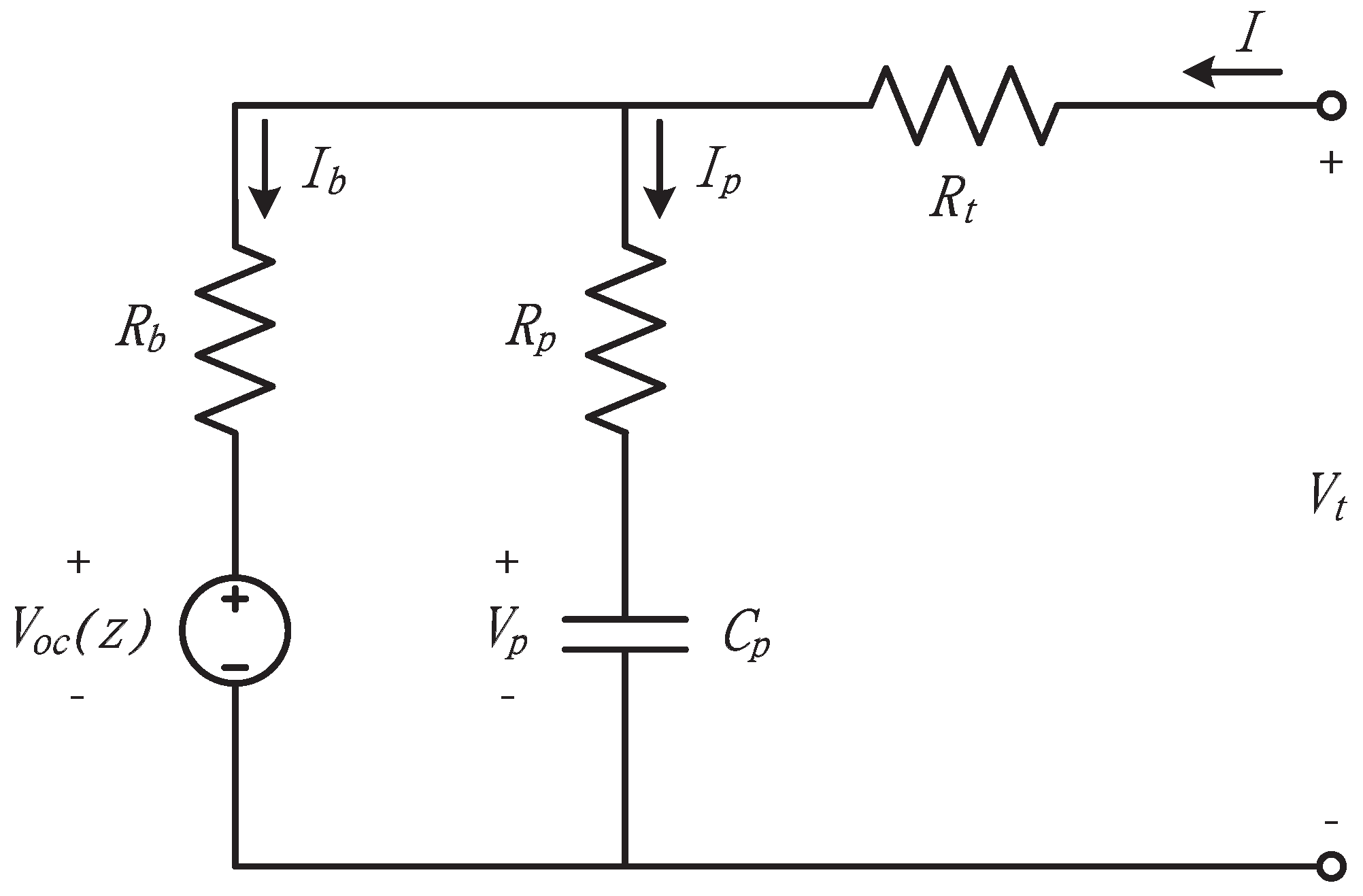
2. Equivalent Circuit-Based Battery Model

In this paper, the dynamic equivalent circuit-based model depicted in Figure 1 is employed because it can accurately represent the behavior of a Li-ion battery with a simple equivalent circuit [10,11,14,15]. This model considers the nonlinear open-circuit voltage (OCV) characteristic and consists of a voltage source $V_{\text{oc}}\left(Z\right)$, a capacitor $C_{\text{p}}$ and three resistors $R_{\text{b}}$, $R_{\text{p}}$ and $R_{\text{t}}$. The voltage source $V_{\text{oc}}\left(Z\right)$ is a function of SOC Z and represents the OCV, which is defined as the terminal voltage of the battery when no load is applied. The capacitor $C_{\text{p}}$ describes the polarization effect of the battery. Resistors $R_{\text{b}}$, $R_{\text{p}}$ and $R_{\text{t}}$ represent a propagation resistor, a diffusion resistor and a terminal resistor, respectively. With three state variables—the terminal voltage $V_{\text{t}}$, the SOC Z and the polarization voltage $V_{\text{p}}$—the state-space equations for the Li-ion battery are obtained as:

$$\begin{array}{c}{\dot{x}}_1=-a_{11}{x}_1+a_{12}{V}_{\text{oc}}\left(x_2\right)+b_{1}u\\ {\dot{x}}_2=-a_2{V}_{\text{oc}}\left(x_2\right)+a_2{x}_3+b_{2}u\\ {\dot{x}}_3=a_3{V}_{\text{oc}}\left(x_2\right)-a_3{x}_3+b_{3}u\\ y=x_1\end{array}$$

(1)

where:

$$\begin{array}{c}\hfill \begin{array}{c}x={\left[V_{t}Z{V}_{\text{p}}\right]}^T,u=I\\ a_{11}=\frac{1}{R_{\text{b}}(R_{\text{b}}+R_{\text{p}})}(\frac{R_{\text{b}}}{C_{\text{p}}}-\frac{R_{\text{p}}}{C_{\text{n}}})\\ a_{12}=\frac{1}{{(R_{\text{b}}+R_{\text{p}})}^2}(\frac{R_{\text{b}}}{C_{\text{p}}}-\frac{R_{\text{p}}}{C_{\text{n}}}-\frac{R_{\text{p}}^2}{C_{\text{n}}{R}_{\text{b}}}+\frac{R_{\text{p}}}{C_{\text{p}}})\\ a_2=\frac{1}{C_{\text{n}}(R_{\text{b}}+R_{\text{p}})},a_3=\frac{1}{C_{\text{p}}(R_{\text{b}}+R_{\text{p}})}\\ b_1=\frac{1}{{(R_{\text{b}}+R_{\text{p}})}^2}\left\{\right(R_{\text{p}}+R_{\text{t}}+\frac{R_{\text{p}}{R}_{\text{t}}}{R_{\text{b}}}\left)\right(\frac{R_{\text{b}}}{C_{\text{p}}}-\frac{R_{\text{p}}}{C_{\text{n}}})+\frac{R_{\text{p}}^2}{C_{\text{n}}}+\frac{R_{\text{b}}^2}{C_{\text{p}}}\}\\ b_2=\frac{R_{\text{p}}}{C_{\text{n}}(R_{\text{b}}+R_{\text{p}})},b_3=\frac{R_{\text{b}}}{C_{\text{p}}(R_{\text{b}}+R_{\text{p}})}\end{array}\end{array}$$

and $C_{\text{n}}$ is the nominal capacitance, which is defined as the value of ampere-hours that can be drawn when the battery goes from $100\%$ SOC to $0\%$ SOC at room temperature.

Figure 1. Equivalent circuit-based battery model.

Figure 1. Equivalent circuit-based battery model.

To verify the observability of the system in Equation (1), the rank of the observability matrix is investigated, and it has a full rank, because the values of the parameters in the battery model are non-zero [14].

3. Two Sliding Mode Approaches for State-of-Charge Estimation

3.1. Conventional Sliding Mode Observer

With the consideration of model uncertainty, the Li-ion battery model in Equation (1) can be written as:

$$\begin{array}{c}\hfill \begin{array}{c}{\dot{x}}_1=-a_{11}{x}_1+a_{12}{V}_{\text{oc}}\left(x_2\right)+b_{1}u+\Delta d_1\hfill \\ {\dot{x}}_2=-a_2{V}_{\text{oc}}\left(x_2\right)+a_2{x}_3+b_{2}u+\Delta d_2\hfill \\ {\dot{x}}_3=a_3{V}_{\text{oc}}\left(x_2\right)-a_3{x}_3+b_{3}u+\Delta d_3\hfill \end{array}\end{array}$$

(2)

where $\Delta d_i$ denotes the uncertainties introduced by modeling and linearization errors, which satisfy the following bounded condition $|\Delta d_i|<{ϵ}_i$ where i = 1, 2, 3.

In the conventional SMO [14], the observer for the terminal voltage $V_{\text{t}}$ is described by:

$$\begin{array}{c}\hfill {\dot{\widehat{x}}}_1=-a_{11}{\widehat{x}}_1+a_{12}{V}_{\text{oc}}\left({\widehat{x}}_2\right)+b_{1}u+k_1\text{sgn}\left(e_1\right)\end{array}$$

(3)

where $e_1=x_1-{\widehat{x}}_1$; $k_1$ is an observer gain for the terminal voltage estimation, and sgn is the sign function defined as:

$$\begin{array}{c}\hfill \text{sgn}\left(e_1\right)=\left\{\begin{array}{cc}1\hfill & \hfill \mathrm{if}{e}_1>0\\ -1\hfill & \hfill \mathrm{if}{e}_1<0\end{array}\right.\end{array}$$

(4)

The switching gain $k_1$ should be selected to guarantee the convergence of the estimation error to zero ($e_1\to 0$). The equation with respect to ${\dot{e}}_1$ is obtained from Equations (1) and (2):

$$\begin{array}{c}\hfill {\dot{e}}_1=-a_{11}{e}_1+a_{12}(V_{\text{oc}}\left(x_2\right)-V_{\text{oc}}\left({\widehat{x}}_2\right)+\Delta d_1-k_1\text{sgn}\left(e_1\right)\end{array}$$

(5)

Consider the following Lyapunov candidate function:

$$\begin{array}{c}\hfill V_1=\frac{1}{2}{e}_1^2\end{array}$$

(6)

The time derivative of the Lyapunov function $V_1$ then becomes:

$$\begin{array}{c}\hfill {\dot{V}}_1=e_1·{\dot{e}}_1\end{array}$$

(7)

Then, suppose the following two cases:

Case (1): Assume $e_1>0$. If the observer gain $k_1$ satisfies:

$$\begin{array}{c}\hfill k_1>|a_{12}(V_{\text{oc}}\left(x_2\right)-V_{\text{oc}}\left({\widehat{x}}_2\right)|+{ϵ}_1\end{array}$$

(8)

then ${\dot{e}}_1<0$, and this also guarantees ${\dot{V}}_1=e_1·{\dot{e}}_1<0$.

Case (2): Assume $e_1<0$. If $k_1$ is chosen to satisfy the condition in Equation (8) as Case 1, then ${\dot{V}}_1<0$. Therefore, with bounded initial estimation error, the mismatch between terminal voltage $V_{\text{t}}$ and its estimate ${\widehat{V}}_{\text{t}}$ is reduced to zero. After sliding mode occurs, ${\dot{e}}_1=e_1=0$ is obtained using the equivalent control concept [26]. The sliding mode equation is then derived from Equation (5):

$$\begin{array}{c}\hfill V_{\text{oc}}\left(x_2\right)-V_{\text{oc}}\left({\widehat{x}}_2\right)={\left\{\frac{k_1}{a_{12}}\text{sgn}\left(e_1\right)\right\}}_{\text{eq}}\end{array}$$

(9)

Next, the observers for the SOC Z are derived as:

$$\begin{array}{c}\hfill {\dot{\widehat{x}}}_2=-a_2{V}_{\text{oc}}\left({\widehat{x}}_2\right)+a_2{\widehat{x}}_3+b_{2}u+k_2\text{sgn}(x_2-{\widehat{x}}_2)\end{array}$$

(10)

where $k_2$ is an observer gain for SOC estimation. Then, the error dynamics of the SOC is obtained by:

$$\begin{array}{c}\hfill {\dot{e}}_2=-a_2\left(V_{\text{oc}}\left(Z\right)-V_{\text{oc}}\left(\widehat{Z}\right)\right)+a_2{e}_3+\Delta d_2-k_2\text{sgn}\left(e_2\right)\end{array}$$

(11)

where $e_i=x_i-{\widehat{x}}_i$, $i=2,3$. With the consideration of a piecewise linear relation between the OCV and the SOC, which is expressed as $V_{\text{oc}}\left(Z\right)=\kappa Z+\nu$, Equation (11) can be rewritten as follows:

$$\begin{array}{c}\hfill {\dot{e}}_2=-a_2\kappa e_2+a_2{e}_3+\Delta d_2-k_2\text{sgn}\left(e_2\right)\end{array}$$

(12)

where κ is not a constant, but varies depending on the SOC [14,15].

In the same manner, we can prove the convergence of SOC error by choosing the Lyapunov candidate function $V_2=1/2e_2^2$ and selecting the observer gain $k_2>{ϵ}_2$. After that, the error equation for $e_3$ can be also derived using the equivalent control concept (i.e., ${\dot{e}}_2=0$ and $e_2=0$) as:

$$\begin{array}{c}\hfill e_3={\left\{\frac{k_2}{a_2}\text{sgn}\left(e_2\right)\right\}}_{\text{eq}}=\left[\frac{k_2}{a_2}\text{sgn}\right({\left\{\frac{k_1}{a_{12}\kappa }\text{sgn}\left(e_1\right)\right\}}_{\text{eq}}){]}_{\text{eq}}\end{array}$$

(13)

Finally, the observer for $V_{\text{p}}$ is designed as:

$$\begin{array}{c}\hfill {\dot{\widehat{x}}}_3=a_3{V}_{\text{oc}}\left({\widehat{x}}_2\right)-a_3{\widehat{x}}_3+b_{3}u+k_3\text{sgn}(x_3-{\widehat{x}}_3)\end{array}$$

(14)

Then, the error equation is given by:

$$\begin{array}{c}\hfill {\dot{e}}_3=a_3\kappa e_2-a_3{e}_{\text{p}}+\Delta d_3-k_3\text{sgn}\left(e_3\right)\end{array}$$

(15)

As in the two cases’ observers, the $V_{\text{p}}$ error converges to zero if the observer gain $k_3$ is larger than ${ϵ}_3$.

In summary, according to the equivalent control concept, the observers for terminal voltage, the SOC Z and the polarization voltage $V_{\text{p}}$ are derived as:

$$\begin{array}{c}\hfill \begin{array}{c}{\dot{\widehat{x}}}_1=-a_{11}{\widehat{x}}_1+a_{12}{V}_{\text{oc}}\left({\widehat{x}}_2\right)+b_{1}u+k_1\text{sgn}\left(e_1\right)\\ {\dot{\widehat{x}}}_2=-a_2{V}_{\text{oc}}\left({\widehat{x}}_2\right)+a_2{\widehat{x}}_3+b_{2}u\\ +k_2\text{sgn}\left({\left\{\frac{k_1}{a_{12}\kappa }\text{sgn}\left(e_1\right)\right\}}_{\text{eq}}\right)\\ {\dot{\widehat{x}}}_3=a_3{V}_{\text{oc}}\left({\widehat{x}}_2\right)-a_3{\widehat{x}}_3+b_{3}u\\ +k_3\text{sgn}\left(\right[\frac{k_2}{a_2}\text{sgn}({\left\{\frac{k_1}{a_{12}\kappa }\text{sgn}\left(e_1\right)\right\}}_{\text{eq}}\left){]}_{\text{eq}}\right)\end{array}\end{array}$$

(16)

Proof: A more detailed proof can be found given in [14].

However, the discontinuous sign function sgn(·) may result in undesired oscillations known as the chattering phenomenon [16]. In addition, the gain $k_i$ should be large enough to satisfy the condition in Equation (8), because the bound is difficult to know in a practical application. This large gain may increase the amplitude of chattering oscillations.

3.2. Adaptive Gain Sliding Mode Observer

In [15], an adaptive gain SMO for SOC estimation was proposed as follows:

$$\begin{array}{c}\hfill \begin{array}{c}{\dot{\widehat{x}}}_1=-a_{11}{\widehat{x}}_1+a_{12}{V}_{\text{oc}}\left({\widehat{x}}_2\right)+b_{1}u+{\widehat{k}}_1\text{sgn}\left(e_1\right)\\ {\dot{\widehat{x}}}_2=-a_2{V}_{\text{oc}}\left({\widehat{x}}_2\right)+a_2{\widehat{x}}_3+b_{2}u+{\widehat{k}}_2\text{sgn}\left(e_2\right)\\ {\dot{\widehat{x}}}_3=a_3{V}_{\text{oc}}\left({\widehat{x}}_2\right)-a_3{\widehat{x}}_3+b_{3}u+{\widehat{k}}_3\text{sgn}\left(e_3\right)\end{array}\end{array}$$

(17)

where ${\widehat{k}}_1$, ${\widehat{k}}_2$ and ${\widehat{k}}_3$ are the adaptive gains and $e_i=x_i-{\widehat{x}}_i$. In this approach, the switching gains of SMO are adapted by the following adaptation laws:

$$\begin{array}{c}\hfill \begin{array}{c}{\dot{\widehat{k}}}_1={\gamma }_1\left|e_1\right|\\ {\dot{\widehat{k}}}_2={\gamma }_2\left|e_2\right|\\ {\dot{\widehat{k}}}_3={\gamma }_3\left|e_3\right|\end{array}\end{array}$$

(18)

where ${\gamma }_1$, ${\gamma }_2$ and ${\gamma }_3$ are positive constants for determining the convergence rate of the gains $k_i$. It is clear that a large ${\gamma }_i$ will force the state variables to converge to the sliding surface at a high speed. However, this adaptation law is only applicable to ideal sliding mode. In the real sliding mode case, $|e_i|$ cannot reach exactly zero in finite time due to finite switching frequency. Thus, the adaptive gains ${\widehat{k}}_i$ are always increasing, and the over-estimated gains may induce larger chattering. Therefore, in this method, the adaptive gains ${\widehat{k}}_i$ should be calibrated regularly.

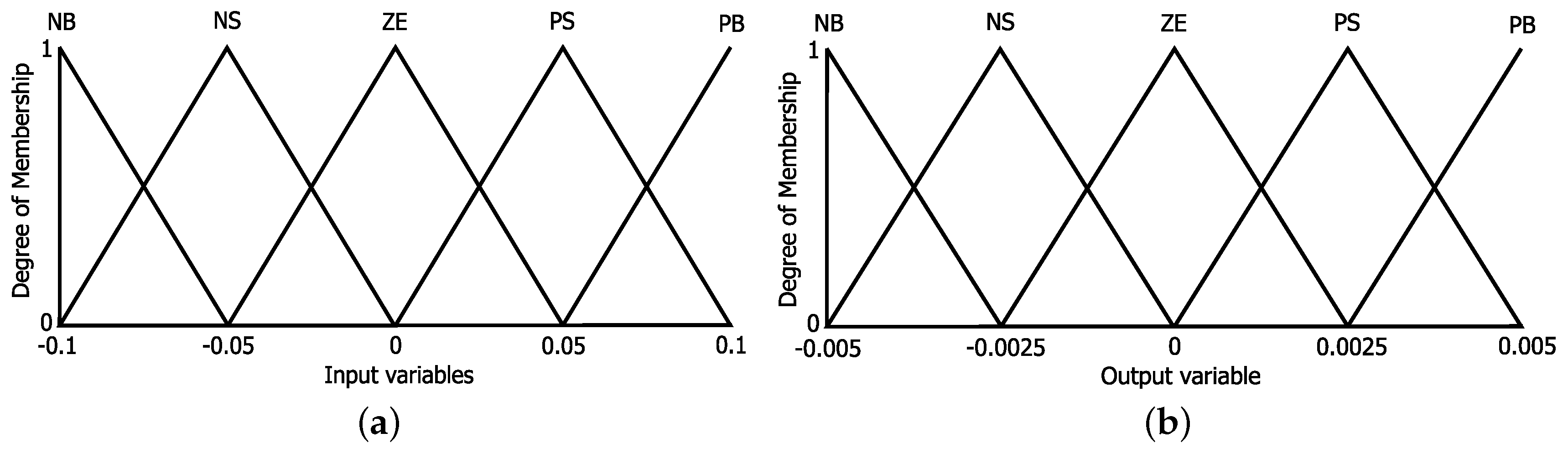
4. Fuzzy Sliding Mode Observer with Grey Prediction

In this paper, we propose the GP-FSMO for SOC estimation. The proposed method employs a grey predictor to forecast a future value of terminal voltage. The predicted error obtained from the predicted terminal voltage is then used instead of the time derivative of the estimation error. Finally, the gains of the SMO are adjusted using a fuzzy inference system.

4.1. Grey Prediction for the Terminal Voltage of a Li-Ion Battery

For grey prediction, the grey model $GM(1,1)$, which consists of a first-order difference equation with one input variable, is commonly used [27]. The establishing procedure of $GM(1,1)$ is described as follows.

Assume that the non-negative original data sequence is defined as:

$$\begin{array}{c}\hfill X^{\left(0\right)}=\{x^{\left(0\right)}\left(1\right),x^{\left(0\right)}\left(2\right),\dots ,x^{\left(0\right)}\left(n\right)\},n\ge 4\end{array}$$

(19)

To weaken the randomness, the original data are converted to monotonically-increasing data, $X^{\left(1\right)}$, using the AGO:

$$\begin{array}{c}\hfill X^{\left(1\right)}=\{x^{\left(1\right)}\left(1\right),x^{\left(1\right)}\left(2\right),\dots ,x^{\left(1\right)}\left(n\right)\},x^{\left(1\right)}\left(1\right)=x^{\left(0\right)}\left(1\right)\end{array}$$

(20)

where:

$$\begin{array}{c}\hfill x^{\left(1\right)}\left(k\right)=\{\sum _{i=1}^k{x}^{\left(0\right)}\left(i\right),k=2,3,\dots ,n\}\end{array}$$

The $GM(1,1)$ model can be constructed by establishing a grey differential equation as [28]:

$$\begin{array}{c}\hfill x^{\left(0\right)}\left(k\right)+a{z}^{\left(1\right)}\left(k\right)=b,k=2,3,\dots ,n\end{array}$$

(21)

where $z^{\left(1\right)}\left(k\right)$ is a newly-defined variable called the background value, which is obtained by the adjacent neighbor mean:

$$\begin{array}{c}\hfill z^{\left(1\right)}\left(k\right)=\frac{1}{2}{x}^{\left(1\right)}\left(k\right)+\frac{1}{2}{x}^{\left(1\right)}(k-1),k=2,3,\dots ,n\end{array}$$

(22)

From Equation (21), the constant coefficients a and b can be estimated using the least square method as:

$$\begin{array}{c}\hfill \widehat{\theta }={\left(B^{T}B\right)}^{-1}{B}^{T}T\end{array}$$

(23)

where:

$$\begin{array}{c}\hfill Y=\left[\begin{array}{c}{x}^{\left(0\right)}\left(2\right)\\ x^{\left(0\right)}\left(3\right)\\ ⋮\\ x^{\left(0\right)}\left(4\right)\end{array}\right],B=\left[\begin{array}{cc}-z^{\left(1\right)}\left(2\right)& 1\\ -z^{\left(1\right)}\left(3\right)& 1\\ ⋮\\ -z^{\left(1\right)}\left(4\right)& 1\end{array}\right],\widehat{\theta }=\left[\begin{array}{c}a\\ b\end{array}\right]\end{array}$$

After then, the first-order differential equation is established for future prediction:

$$\begin{array}{c}\hfill \frac{\text{d}{x}^{\left(1\right)}}{\text{d}t}+a{x}^{\left(1\right)}=b\end{array}$$

(24)

Equation (24) is called a reflection or reflection whitenization equation because it can reflect the exponential growth trend of the sequence $X^{\left(1\right)}$.

The solution of Equation (24) is given by:

$$\begin{array}{c}\hfill {\overline{x}}^{\left(1\right)}(k+1)=\left(x^{\left(0\right)}\left(1\right)-\frac{b}{a}\right)e^{-a\left(k\right)}+\frac{b}{a},k=1,2,\dots n\end{array}$$

(25)

where ${\overline{x}}^{\left(1\right)}(k+1)$ represents the predicted value for the AGO sequence of $X^{\left(0\right)}$. Finally, by applying the inverse AGO ($x^{\left(0\right)}\left(k\right)=x^{\left(1\right)}\left(k\right)-x^{\left(1\right)}(k-1)$), we have the prediction for the original data $X^{\left(0\right)}$:

$$\begin{array}{c}\hfill {\overline{x}}^{\left(0\right)}(k+1)={\overline{x}}^{\left(1\right)}(k+1)-{\overline{x}}^{\left(1\right)}\left(k\right)\\ \hfill =\left(x^{\left(0\right)}\left(1\right)-\frac{b}{a}\right)\left(1-e^a\right)e^{-ak},k=1,2,\dots n\end{array}$$

(26)

Note that the detailed proof and description of the $GM(1,1)$ is introduced in [28].

In conclusion, we employ the grey prediction method with the rolling method [29] to obtain the one-step-ahead predictive value of terminal voltage ${\overline{V}}_t(k+1)$ defined as:

$$\begin{array}{c}\hfill {\overline{V}}_{\text{t}}(k+1)=\left(V_{\text{t}}(k-3)-\frac{b}{a}\right)\left(1-e^a\right)e^{-ak}\end{array}$$

(27)

where the coefficients a and b are computed from the measured terminal voltage sequence $V_{\text{t}}\left(k\right),V_{\text{t}}(k-1),V_{\text{t}}(k-2)$ and $V_{\text{t}}(k-3)$ using Equation (23).

Remark 1. To obtain the discrete voltage sequence $V_{\text{t}}\left(k\right),V_{\text{t}}(k-1),V_{\text{t}}(k-2)$ and $V_{\text{t}}(k-3)$, a discrete-time equivalent model described in [10] is adopted in this paper. This model is established under the assumption that the applied input current is constant during each sampling interval.

4.2. Observer Gain Adaptation Law

Consider the first-order SMO Equation (16); the adaptation law for gain ${\widehat{k}}_i$ is designed as:

$$\begin{array}{c}\hfill {\dot{\widehat{k}}}_i=\left\{\begin{array}{cc}\alpha (e_{\text{t}},{\tilde{e}}_{\text{t}})\hfill & \hfill \mathrm{if}{\widehat{k}}_i\ge k_{i,\text{min}}\\ \mu \hfill & \hfill \mathrm{if}{\widehat{k}}_i<k_{i,\text{min}}\end{array}\right.\end{array}$$

(28)

where α is a gain tuning parameter, μ is chosen to be a small positive value, such that the gain $k_i$ satisfies the condition in Equation (8), and $k_{i,\text{min}}$ is a positive number that satisfies $k_{i,\text{min}}>{ϵ}_i$, which is the same condition of the conventional SMO. Finally, the observer gain is obtained by:

$$\begin{array}{c}\hfill \left[\begin{array}{c}{k}_1(k+1)\\ k_2(k+1)\\ k_3(k+1)\end{array}\right]=\left[\begin{array}{c}{k}_1\left(k\right)\\ k_2\left(k\right)\\ k_3\left(k\right)\end{array}\right]+\alpha \left[\begin{array}{c}{\beta }_1\\ {\beta }_2\\ {\beta }_3\end{array}\right]\end{array}$$

(29)

where ${\beta }_1,{\beta }_2$ and ${\beta }_3$ are the step size coefficients, which are designed to set the rate of gain adaptation. In this paper, we choose ${\beta }_1={\beta }_3=1$ and ${\beta }_2=0.5$ to reflect the property of terminal voltage and SOC. From a physical point of view, the SOC varies more slowly than the terminal voltage under the operation of the battery.

The gain tuning parameter α is determined through a fuzzy inference system in order to simultaneously improve tracking performance and reduce chattering. The input variables of the fuzzy inference system are chosen as estimation error $e_t$ and one-step ahead prediction error ${\tilde{e}}_t$. The estimation error at the k-th sampling instant is defined as:

$$\begin{array}{c}\hfill e_{\text{t}}\left(k\right)=V_{\text{t}}\left(k\right)-{\widehat{V}}_{\text{t}}\left(k\right)\end{array}$$

(30)

and the one-step-ahead prediction error is calculated from Equation (27) as:

$$\begin{array}{c}\hfill {\tilde{e}}_{\text{t}}(k+1)={\overline{V}}_{\text{t}}(k+1)-{\widehat{V}}_{\text{t}}(k+1)\end{array}$$

(31)

where ${\widehat{V}}_{\text{t}}(k+1)$ is the estimated terminal voltage from the GP-FSMO and ${\overline{V}}_{\text{t}}(k+1)$ the one-step-ahead predictive value of terminal voltage from the grey predictor.

The fuzzy rules of the fuzzy inference system are generated from the following simple idea. First, if the one-step-ahead prediction error becomes greater than the current estimation error (i.e., ${\tilde{e}}_{\text{t}}(k+1)>e_{\text{t}}\left(k\right)$), the gain $k_i$ should be increased to prevent the destruction of the sliding mode. Conversely, when the one-step-ahead prediction error becomes smaller than the current estimation error (i.e., ${\tilde{e}}_{\text{t}}(k+1)<e_{\text{t}}\left(k\right)$), this means the gain is unnecessarily large with respect to the upper bound of uncertainties and the gain should be decreased to reduce chattering. In order to reflect this relationship, the absolute predicted change of error is defined as:

$$\begin{array}{c}\hfill \Delta e_{\text{t}}\left(k\right)=|e_{\text{t}}\left(k\right)|-|{\tilde{e}}_{\text{t}}(k+1)|\end{array}$$

(32)

Thus, the estimation error $e_{\text{t}}\left(k\right)$ and absolute predicted change of error $\Delta e_{\text{t}}\left(k\right)$ are selected as input variables to the fuzzy inference system. The triangular type of membership function, shown in Figure 2, is used for fuzzification of the input variables. The range of the membership functions is designed according to the maximum $e_{\text{t}}\left(k\right)$ and $\Delta e_{\text{t}}\left(k\right)$ that may occur. There are five fuzzy subsets for $e_{\text{t}}$, ${\tilde{e}}_{\text{t}}$ and α: positive big (PB), positive small (PS), zero (ZE), negative small (NS) and negative big (NB).

As shown in Table 1, the set of 21 fuzzy rules is established to represent the relationship between the input and output variables of the fuzzy inference system. Whether the gain is to be increased or decreased is determined based on the fuzzy rules. Here, the range of output variable α is designed to be −0.005 to 0.005.

Remark 2. It should be noted that the proof of the convergence of the GP-FSMO is the same as that of the conventional SMO, because the gains of the GP-FSMO are always selected to satisfy the conditions $k_i\ge k_{i,min},i=1,2,3$. In this paper, $k_{i,min}$ are determined experimentally by comparing the modeling output with the actual output. In practice, the uncertainties $\Delta d_i$ are hard to quantify owing to the complex dynamics of batteries. However, the proposed GP-FSMO is expected to work well, even without knowing the exact value of $k_{i,min}$. Suppose that there exists a positive value $k_i^{*}$ such that $k_i^{*}=\left|d_i\right|,i=1,2,3$. If the gain $k_i$ is adapted through Equation (28) and decreases below $k_i^{*}$ eventually, then the sliding mode will be destroyed and the sliding variable $e_1$ will no longer be zero. After that, the gain $k_i$ increases until the sliding mode is re-established.

Figure 2. Membership functions of the input and output variables for the grey prediction-based fuzzy sliding mode observer (GP-FSMO): (a) membership functions of $e_{\text{t}}\left(k\right)$ and $\Delta e_{\text{t}}\left(k\right)$; (b) membership function of α.

Figure 2. Membership functions of the input and output variables for the grey prediction-based fuzzy sliding mode observer (GP-FSMO): (a) membership functions of $e_{\text{t}}\left(k\right)$ and $\Delta e_{\text{t}}\left(k\right)$; (b) membership function of α.

Table 1. Fuzzy rules for gain tuning parameter α. PB: positive big; PS: positive small; ZE: zero; NS: negative small; and NB: negative big.

$\Delta e_{\text{t}}\left(k\right)$			e
	PB	PS	ZE	NS	NB
PB	NS	-	-	-	NS
PS	NS	NS	-	NS	NS
ZE	NS	ZE	ZE	ZE	NS
NS	PS	PS	PS	PS	PS
NB	PB	PB	PB	PB	PB

Table 1. Fuzzy rules for gain tuning parameter α. PB: positive big; PS: positive small; ZE: zero; NS: negative small; and NB: negative big.

$\Delta e_{\text{t}}\left(k\right)$			e
	PB	PS	ZE	NS	NB
PB	NS	-	-	-	NS
PS	NS	NS	-	NS	NS
ZE	NS	ZE	ZE	ZE	NS
NS	PS	PS	PS	PS	PS
NB	PB	PB	PB	PB	PB

5. Experiment Results

In our experiments, a fresh 18650-type Li-ion battery (LG Chemical Co., Ltd., Seoul, Korea) with 3.0-Ah nominal capacity and 3.75-V nominal voltage was used. The battery test bench consisted of an electrical load, a power supply and a data acquisition device. The electrical load and power supply were used to discharge/charge the battery, and the terminal voltage was measured by the NI9229 voltage measurement module with accuracy of 0.001 V. All experiments were conducted at room temperature, and the sampling interval T is 0.01 s.

Two types of discharge tests for the Li-ion battery were performed: (i) a pulse discharge test; and (ii) a random discharge test. The estimation performance of the proposed method was verified through comparisons with the estimation results of the conventional SMO, the adaptive gain SMO and GP-FSMO. Note that the ampere-hour counting method considering the Coulombic efficiency was used to obtain the reference SOC value.

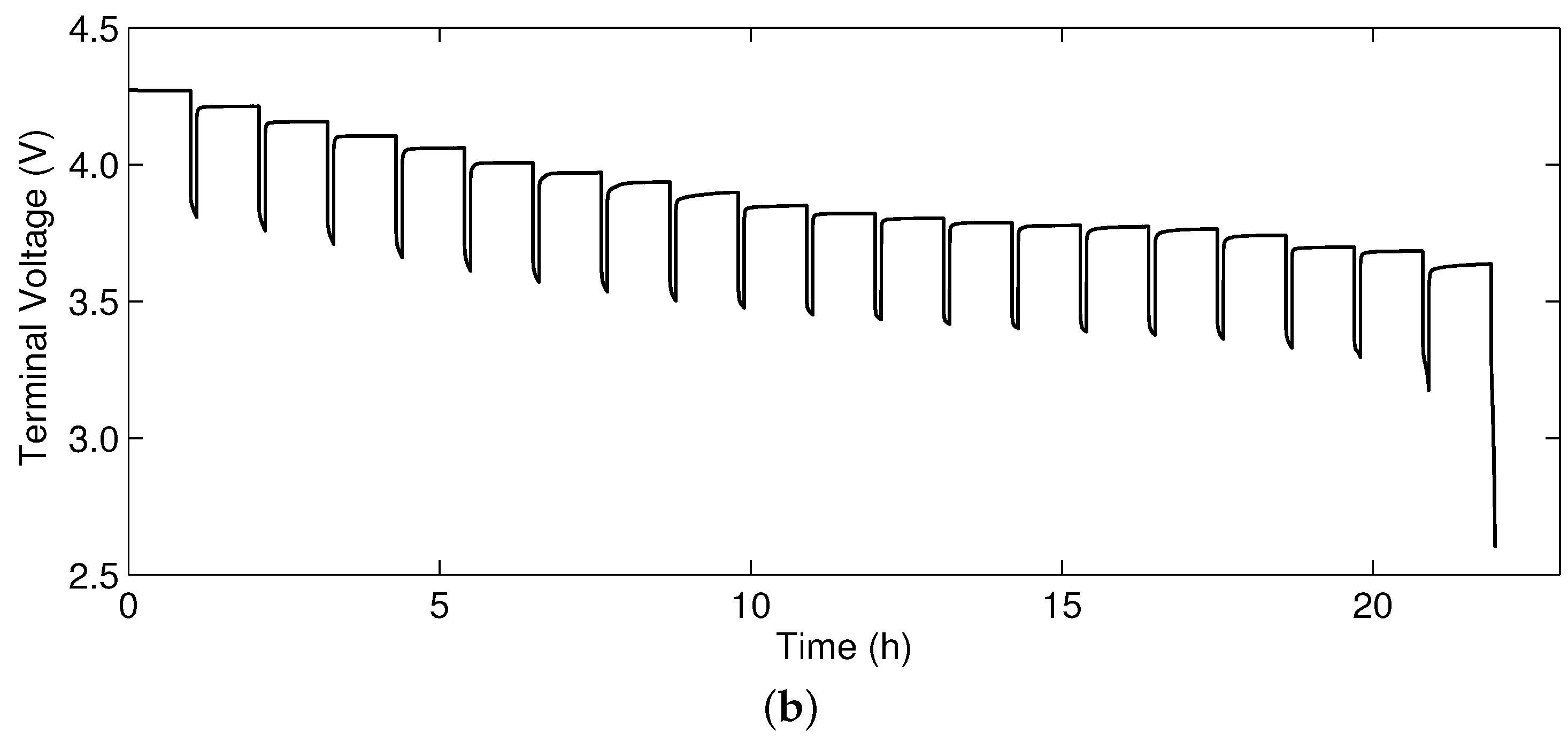
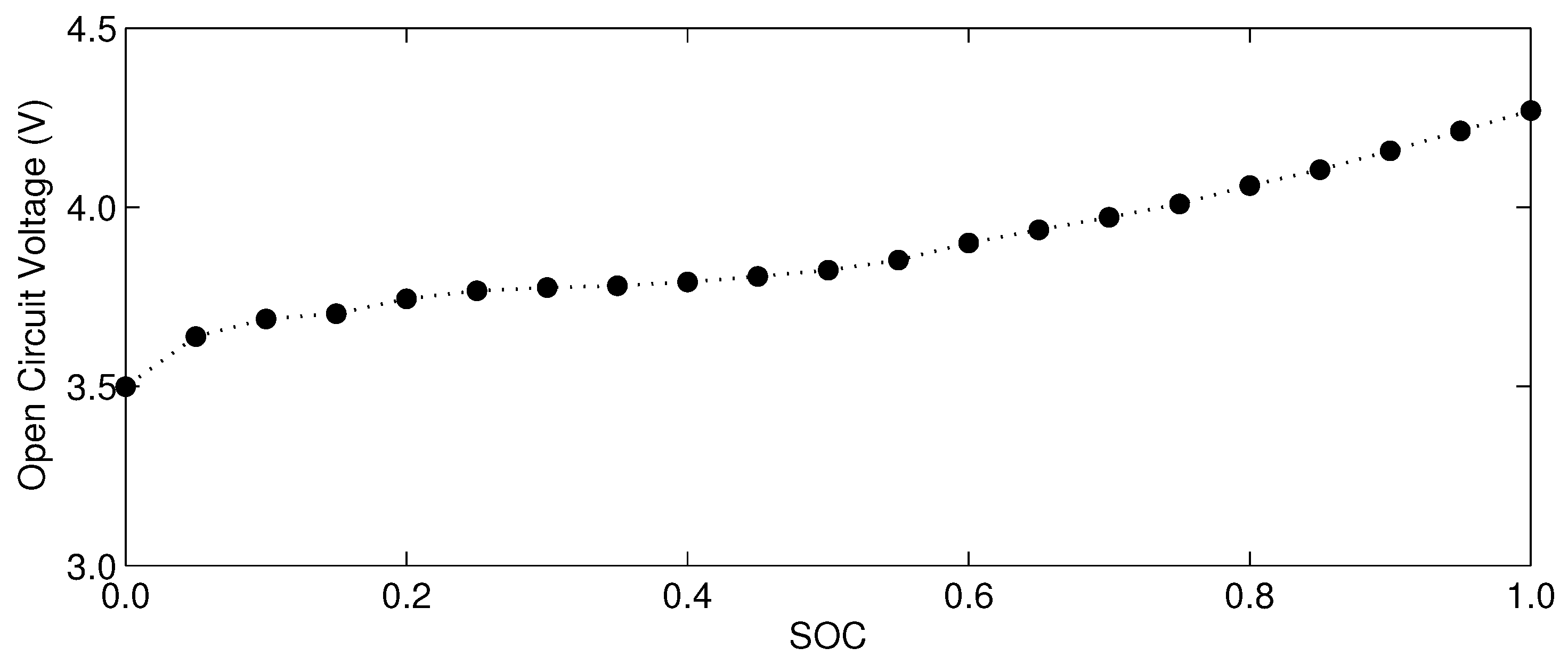
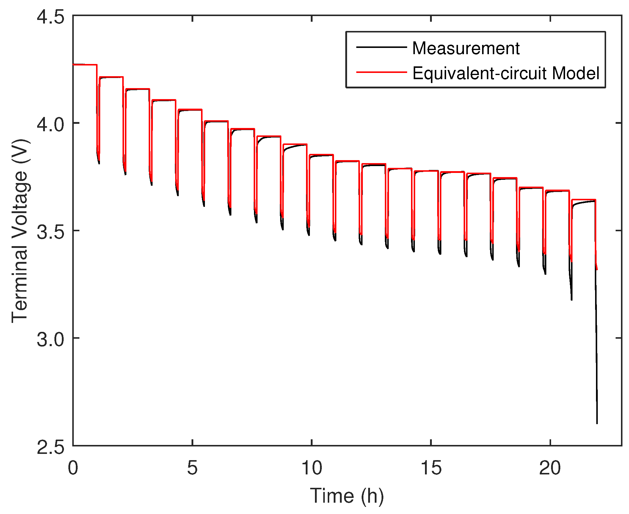
5.1. Parameter Extraction

To determine the parameters of the battery model in Equation (1), the battery characterization test is performed. In this test, 1.0-C discharge pulses in 0.5 s intervals are applied. Using the output voltage of the battery characterization test in Figure 3, the internal resistance $R_{\text{int}}$ is obtained as:

$$\begin{array}{c}\hfill R_{\text{int}}=\frac{V_3-V_2}{I_{\text{dis}}}\end{array}$$

(33)

where $I_{\text{dis}}$ is the discharge current. Then, in general, it is assumed that $R_{\text{b}}$ and $R_{\text{p}}$ are equivalent to 75% of $R_{\text{int}}$ and $R_{\text{t}}$ is equivalent to 25% of $R_{\text{int}}$ [10].

Figure 3. Prediction result of the terminal voltage based on the grey predictor.

Figure 3. Prediction result of the terminal voltage based on the grey predictor.

The polarization capacity $C_{\text{p}}$ is derived from the following equations:

$$\begin{array}{c}\hfill \begin{array}{c}{V}_{\text{no\_load}}=V_1=V_3+(V_4-V_3)(1-e^{-t/\tau })\\ \tau =-\Delta tln(1-\frac{V_4-V_3}{V_1-V_3})\tau =C_{\text{p}}(R_{\text{b}}+R_{\text{p}})\\ \therefore C_{\text{p\_init}}=\frac{\tau }{R_{\text{b}}+R_{\text{p}}}\end{array}\end{array}$$

(34)

The identified parameters of the equivalent circuit based at 100% SOC are determined as:

$$\begin{array}{c}\hfill C_{\text{p}}=17.6735\text{F},R_{\text{b}}=0.165\Omega ,R_{\text{p}}=0.165\Omega ,R_{\text{t}}=0.055\Omega .\end{array}$$

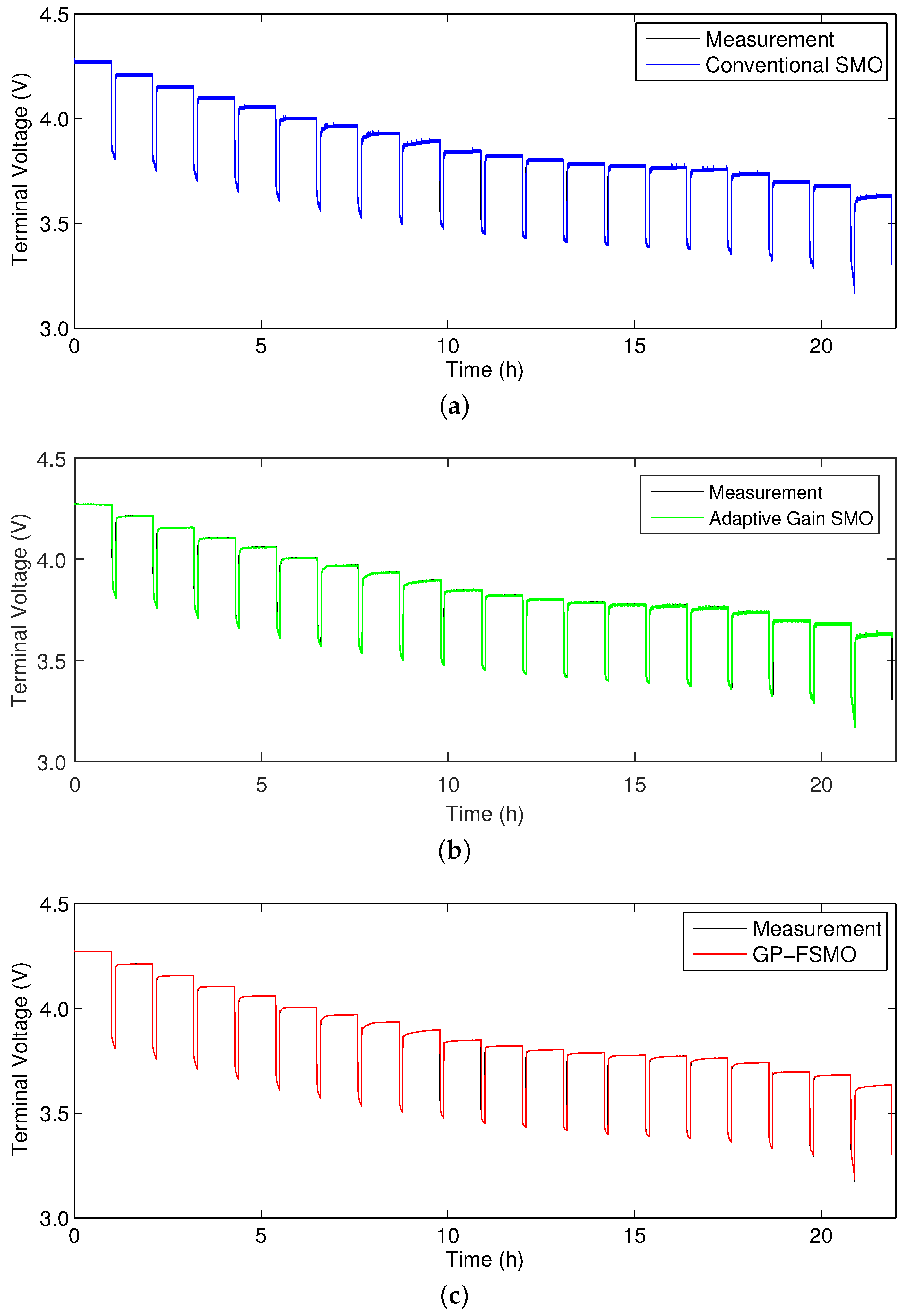
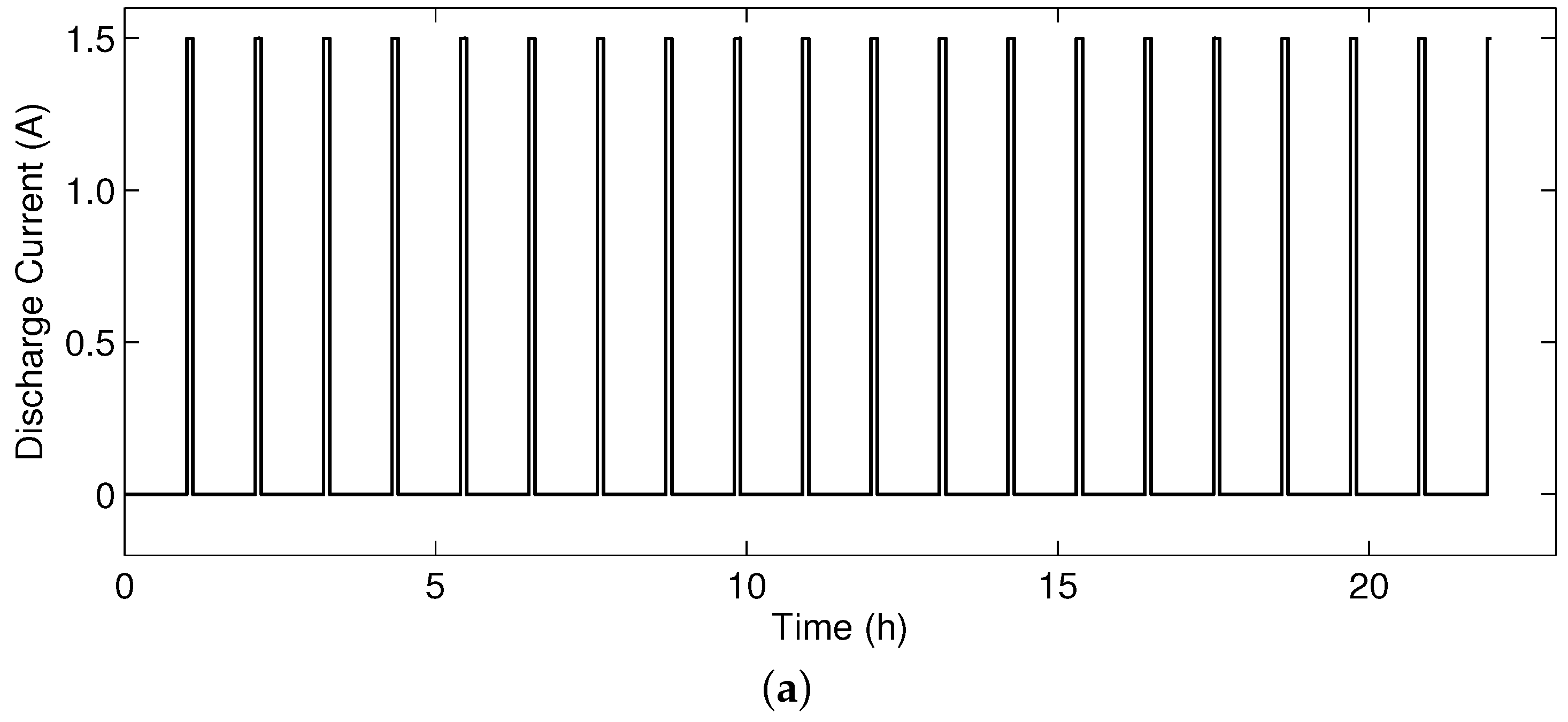
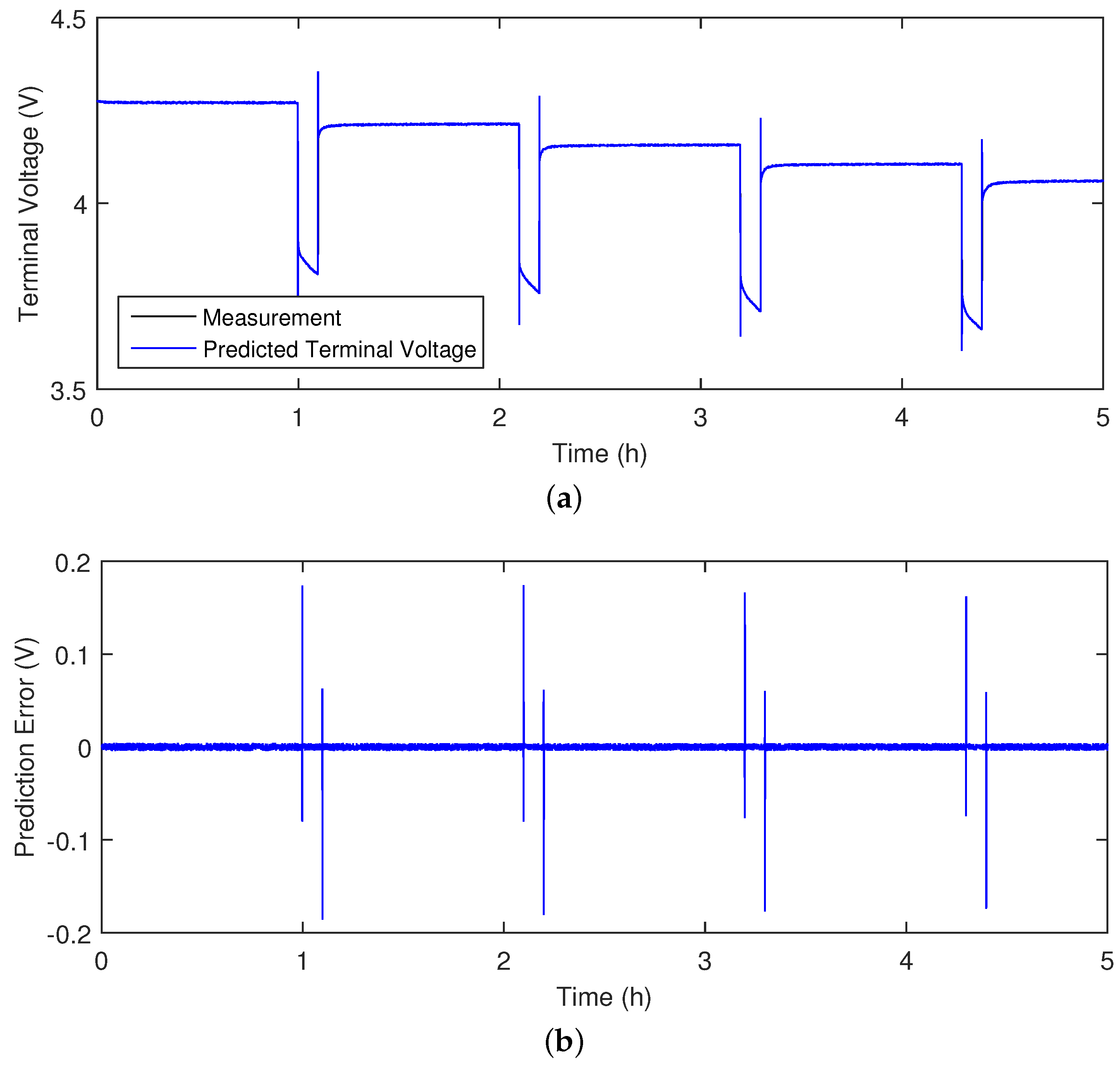
5.2. Pulse Discharge Test

In the first experiment, the fully-charged battery was discharged at 5% SOC intervals with a sequence of 0.5C 360-s discharge pulses and 3600-s rests in the voltage range of 2.6 V to 4.3 V. Figure 4 shows the discharge current profile and terminal voltage. As a result, the OCV-SOC curve in Figure 5 was obtained from the steady-state voltage after each 3600-s rest.

Figure 4. (a) Pulse discharge current profile; and (b) measured terminal voltage.

Figure 4. (a) Pulse discharge current profile; and (b) measured terminal voltage.

Figure 5. Open-circuit voltage (OCV)-state-of-charge (SOC) curve at room temperature.

Figure 5. Open-circuit voltage (OCV)-state-of-charge (SOC) curve at room temperature.

In order to validate the equivalent circuit-based battery model described in Section 2, the curves of the measured terminal voltage and the model-based output voltage are given in Figure 6. It shows that the battery model can accurately describe the terminal voltage in a high SOC range. On the other hand, in a low SOC range, some modeling errors exist, because the parameters are extracted from the battery with 100% SOC. However, this can be compensated by the SMOs used in this paper.

Figure 6. Validation of the equivalent circuit-based battery model.

Figure 6. Validation of the equivalent circuit-based battery model.

In this experiment, the switching gains for the conventional SMO were selected and fixed as:

$$\begin{array}{c}\hfill L_1={[0.020.010.020.1]}^T\end{array}$$

(35)

and the positive constants for the adaptive gain SMO were set small enough as ${\gamma }_1=0.003$, ${\gamma }_2=0.0015$ and ${\gamma }_3=0.003$. The gains for the GP-FSMO were adapted based on the comparison between the estimation error and the prediction error as explained in Section 4. In order to demonstrate the prediction performance of the grey predictor, the grey prediction result for terminal voltage during 0 to 5 h was plotted and is shown in Figure 7. It can be seen that the prediction value is accurate, except in cases when the current changes suddenly. Note that the effect of the impulse prediction error is weakened during the gain adaptation process, because the absolute predicted change of error $\Delta e_{\text{t}}\left(k\right)$ is mapped into a bounded fuzzy variable through the fuzzification stage.

Figure 7. Prediction result of the terminal voltage based on the grey predictor. (a) Predicted terminal voltage; and (b) prediction error.

Figure 7. Prediction result of the terminal voltage based on the grey predictor. (a) Predicted terminal voltage; and (b) prediction error.

The SOC estimation results are depicted in Figure 8. In addition, to provide a clear view, we present the zoomed-in plots of the SOC range of 20% to 40% in Figure 9. As can be seen, the GP-FSMO can estimate the SOC more accurately than the other two methods and enhances the estimation performance in terms of chattering reduction. In contrast, the SOC estimation error for the conventional SMO experiences sudden changes of more than 5%, as well as the chattering phenomenon. In the case of the adaptive gain SMO, the estimated SOC seems to track the reference the SOC well in the beginning. However, the SOC estimation error and the chattering become large, because the switching gain has been over-estimated through Equation (18). To compare the accuracy of three estimation methods, the absolute values of the SOC estimation error at different SOC ranges are shown in Table 2.

Figure 8. Estimation results of SOC in the pulse discharge test: (a) conventional SMO; (b) adaptive gain SMO; and (c) GP-FSMO.

Figure 8. Estimation results of SOC in the pulse discharge test: (a) conventional SMO; (b) adaptive gain SMO; and (c) GP-FSMO.

Table 2. Comparison of SOC estimation error in the pulse discharge test.

SOC range	Error (%)	Methods
		Conventional SMO	Adaptive gain SMO	GP-FSMO
100% to 70%	Maximum	5.89	3.05	2.28
	Mean	2.4	1.36	1.07
70% to 40%	Maximum	6.75	4.97	3.83
	Mean	3.71	2.87	1.92
40% to 5%	Maximum	8.16	5.54	4.11
	Mean	3.73	3.01	1.94

Table 2. Comparison of SOC estimation error in the pulse discharge test.

SOC range	Error (%)	Methods
		Conventional SMO	Adaptive gain SMO	GP-FSMO
100% to 70%	Maximum	5.89	3.05	2.28
	Mean	2.4	1.36	1.07
70% to 40%	Maximum	6.75	4.97	3.83
	Mean	3.71	2.87	1.92
40% to 5%	Maximum	8.16	5.54	4.11
	Mean	3.73	3.01	1.94

Figure 9. Zoomed-in plots of the SOC range of 20% to 40%: (a) conventional SMO; (b) adaptive gain SMO; (c) GP-FSMO; and (d) comparison of the estimation errors between the conventional SMO, adaptive gain SMO and the GP-FSMO.

Figure 9. Zoomed-in plots of the SOC range of 20% to 40%: (a) conventional SMO; (b) adaptive gain SMO; (c) GP-FSMO; and (d) comparison of the estimation errors between the conventional SMO, adaptive gain SMO and the GP-FSMO.

To further evaluate the estimation performance, the estimation results of the terminal voltage between the conventional SMO, adaptive gain SMO and the proposed GP-FSMO are compared in Figure 10. We can see that the terminal voltage estimation results for the conventional SMO include the undesirable chattering phenomenon with an average absolute error of 0.0074 V. Furthermore, the adaptive gain SMO suffers from the over-estimated switching gains, and the terminal voltage estimation error increases gradually to about 0.01 V. On the contrary, the GP-FSMO improves the estimation performance in terms of terminal voltage estimation accuracy and chattering reduction, since the average absolute error is less than 0.002 V.

Figure 10. Estimation results of the terminal voltage in the pulse discharge test: (a) conventional SMO; (b) adaptive Gain SMO; (c) GP-FSMO; and (d) comparison of the estimation errors between the conventional SMO, adaptive gain SMO and GP-FSMO.

Figure 10. Estimation results of the terminal voltage in the pulse discharge test: (a) conventional SMO; (b) adaptive Gain SMO; (c) GP-FSMO; and (d) comparison of the estimation errors between the conventional SMO, adaptive gain SMO and GP-FSMO.

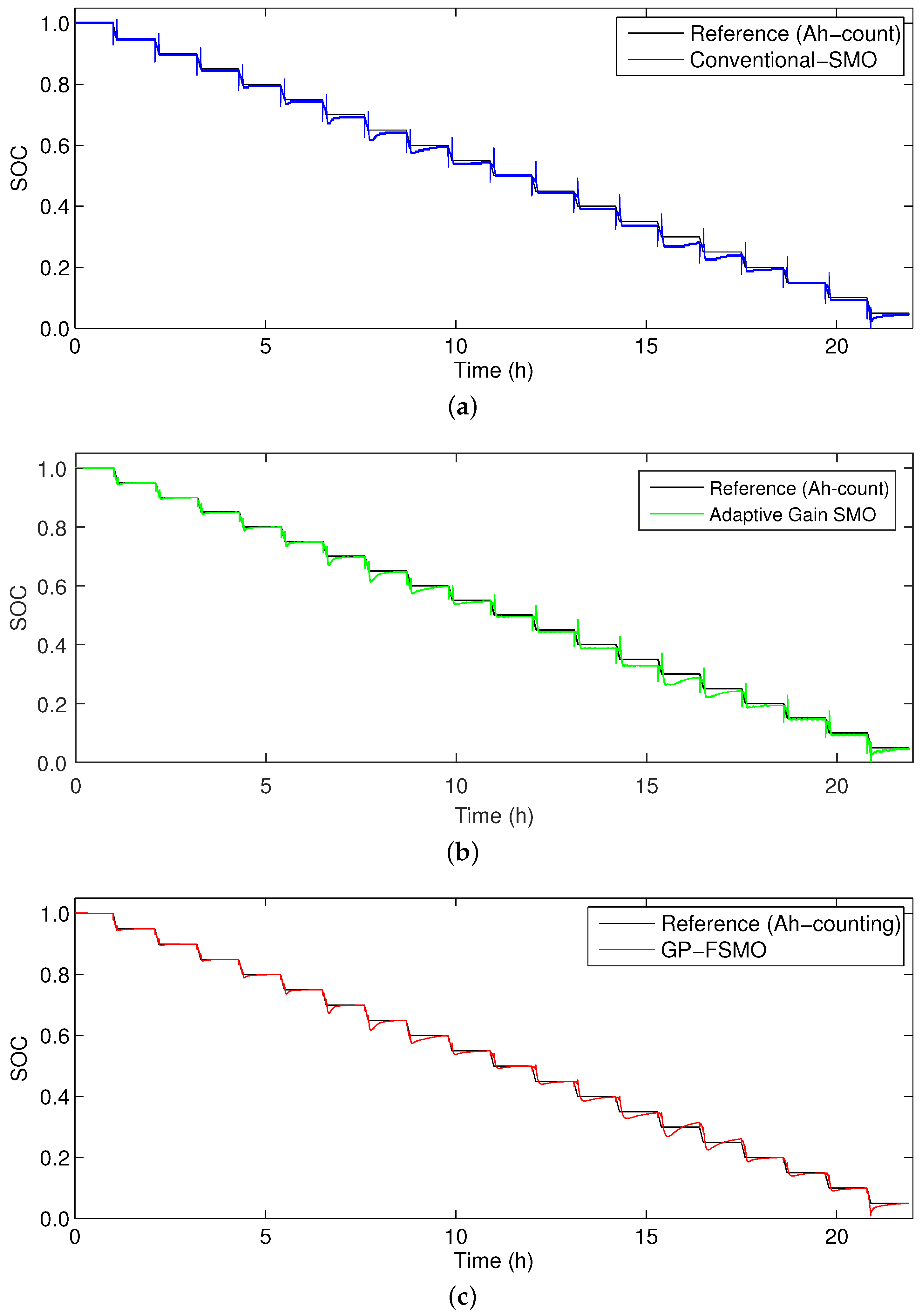
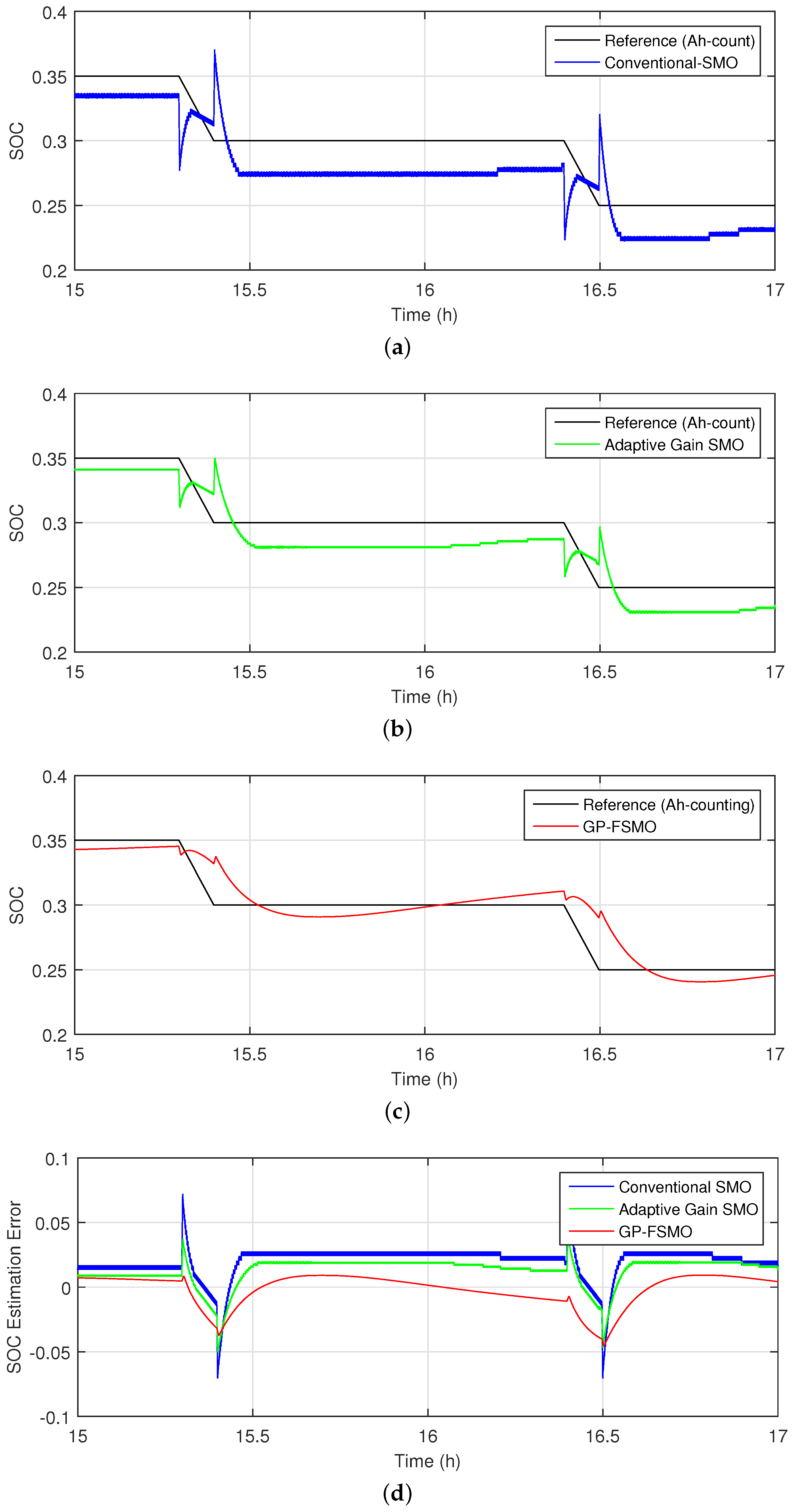
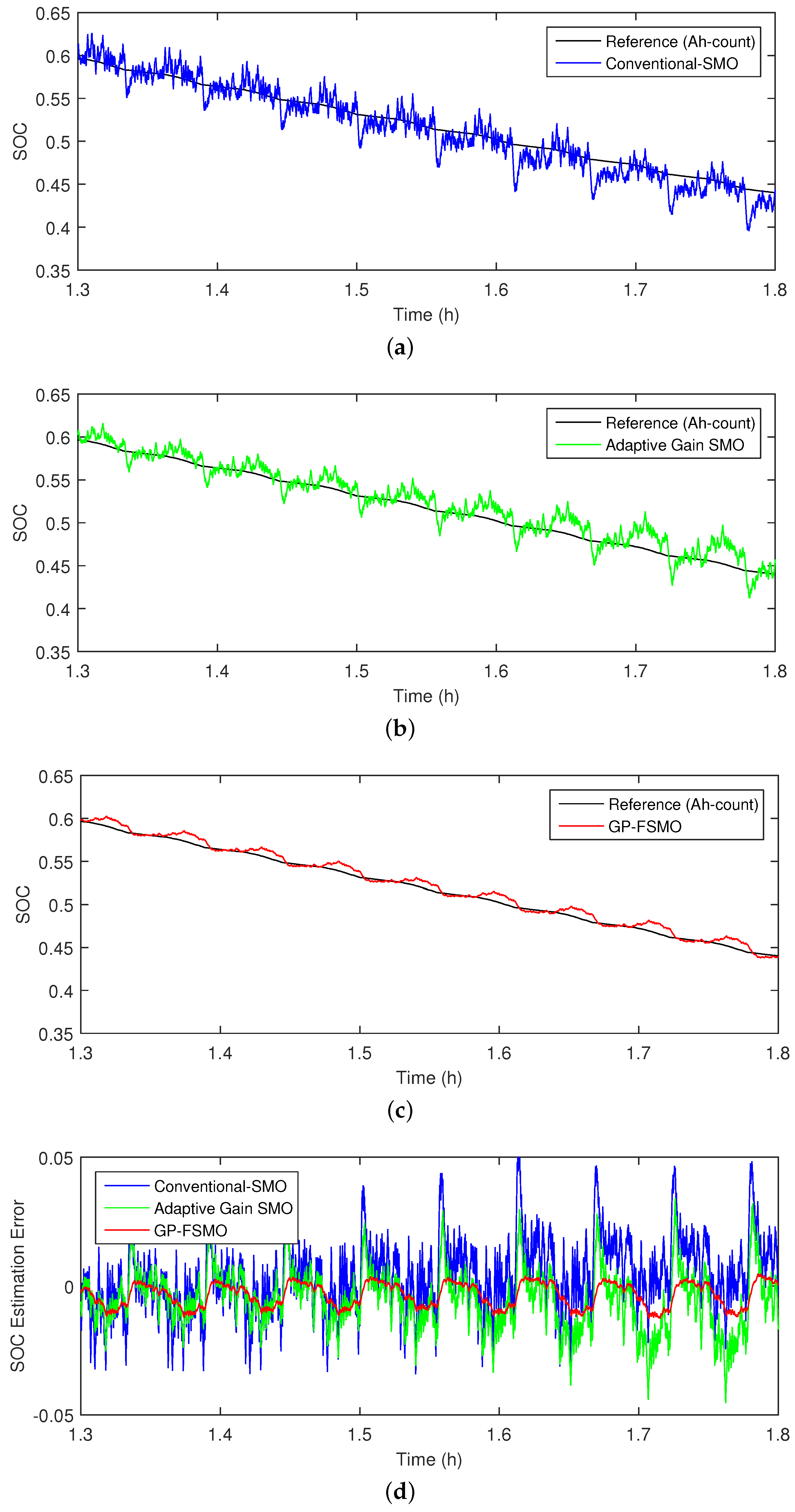
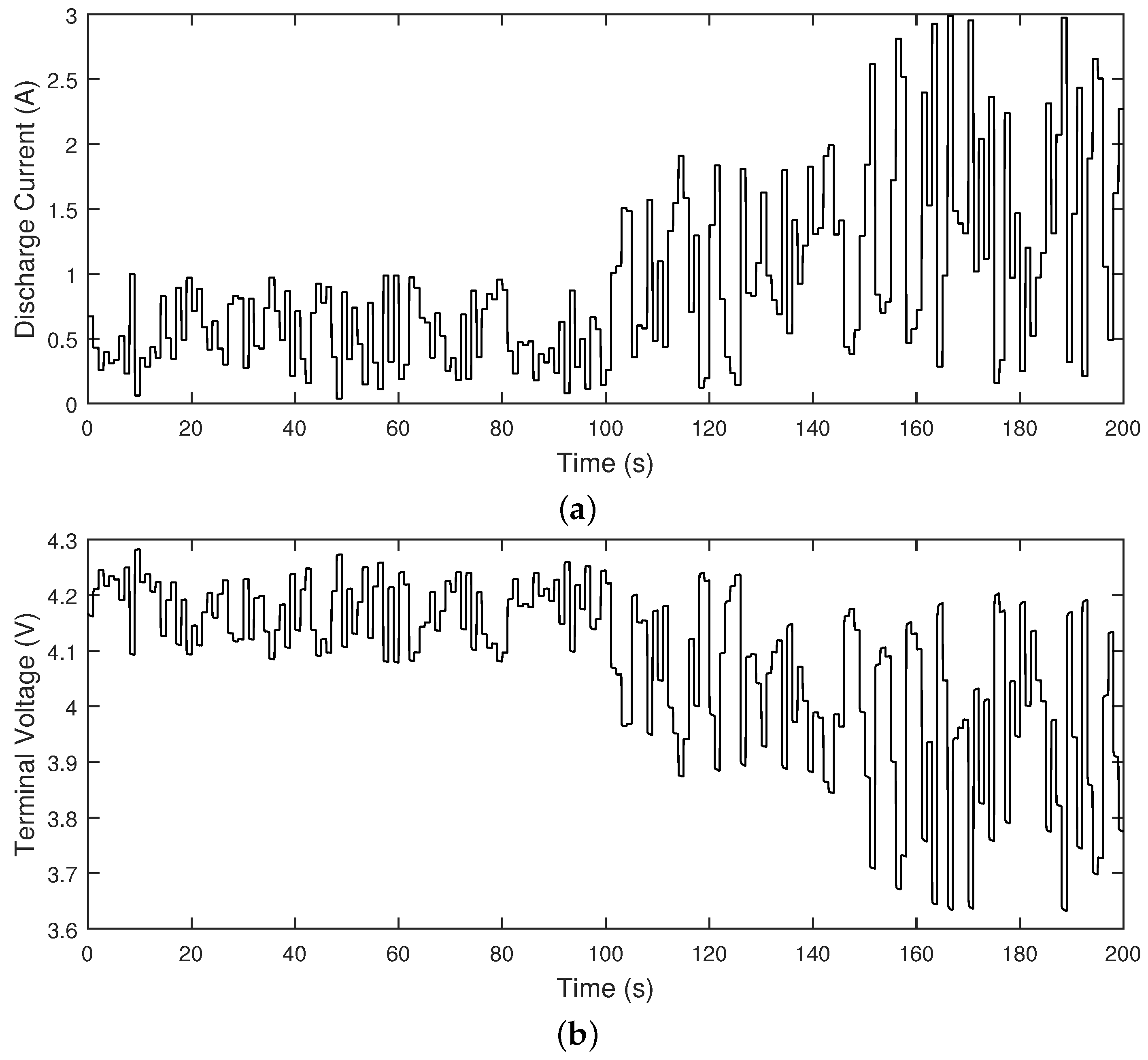
5.3. Random Discharge Current Test

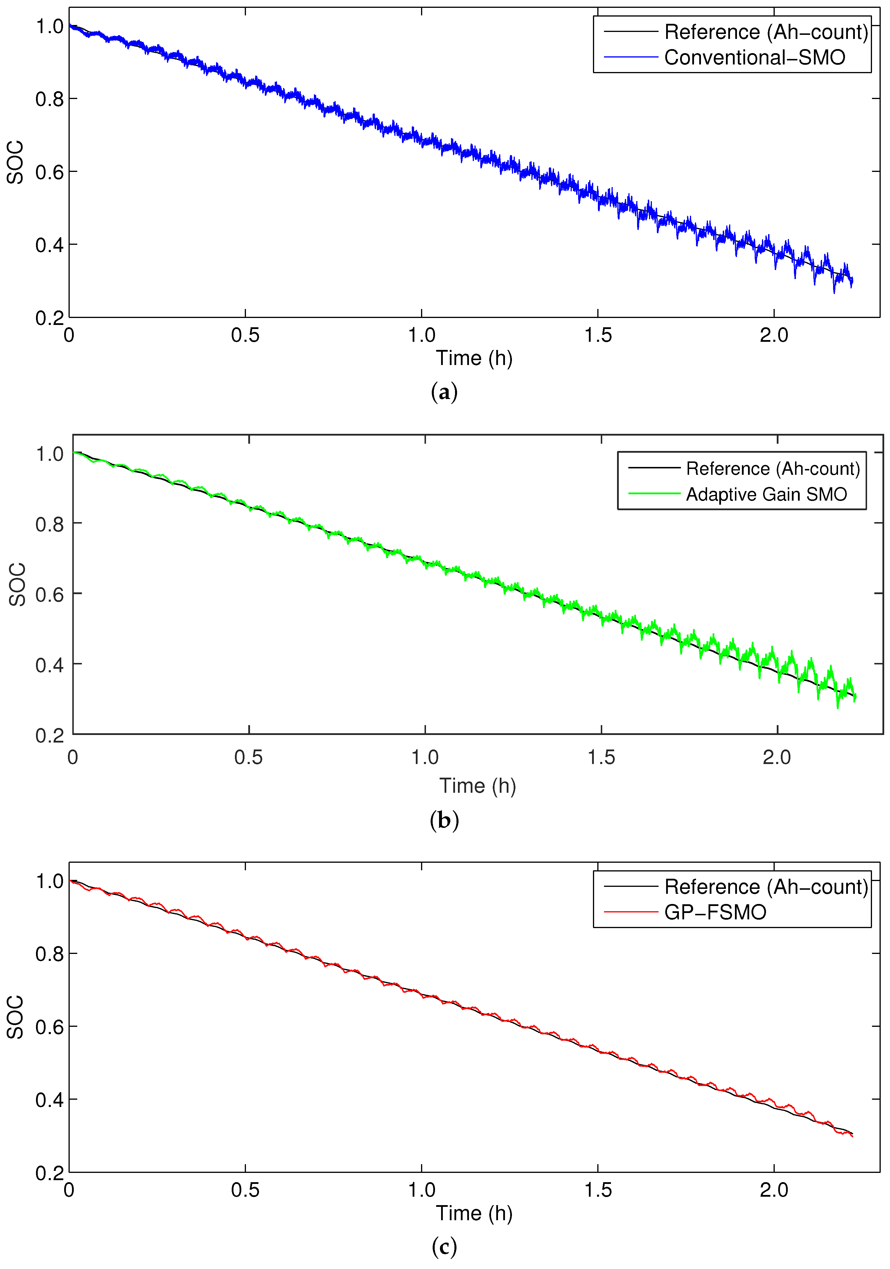
In the second experiment, to describe the real situation of battery usage, the random discharge current in Figure 11 was applied repeatedly 40 times over the 100% to 30% SOC range. For this experiment, it was necessary to increase the gains for the conventional SMO, because the fluctuation in terminal voltage was larger than that in the previous experiment. Thus, the switching gains for the conventional SMO were selected as:

$$\begin{array}{c}\hfill L_2={[0.0350.020.0350.1]}^T\end{array}$$

(36)

Figure 11. (a) Random discharge current profile; (b) measured terminal voltage.

Figure 11. (a) Random discharge current profile; (b) measured terminal voltage.

Figure 12 and Table 3 present the SOC estimation results of the conventional SMO, adaptive gain SMO and GP-FSMO. Furthermore, for a precise and clear comparison of the SOC estimation performance of both methods, zoomed-in plots between 1.3 h and 1.8 h are shown in Figure 13. The estimation error of the conventional SMO exceeds 4% with the chattering phenomenon, and the adaptive gain SMO suffers from the over-estimated switching gains, as expected. On the other hand, we can see that the SOC estimation result of the GP-FSMO accurately follows the reference SOC value with an estimation error of less than 3% and also reduces chattering.

Figure 12. Estimation results of SOC in the random discharge test: (a) conventional SMO; (b) adaptive Gain SMO; and (c) GP-FSMO.

Figure 12. Estimation results of SOC in the random discharge test: (a) conventional SMO; (b) adaptive Gain SMO; and (c) GP-FSMO.

Figure 13. Zoomed-in plots of the SOC range of 35% to 65%: (a) conventional SMO; (b) adaptive gain SMO; (c) GP-FSMO; and (d) comparison of estimation errors between the conventional SMO, adaptive gain SMO and the GP-FSMO.

Figure 13. Zoomed-in plots of the SOC range of 35% to 65%: (a) conventional SMO; (b) adaptive gain SMO; (c) GP-FSMO; and (d) comparison of estimation errors between the conventional SMO, adaptive gain SMO and the GP-FSMO.

Table 3. Comparison of SOC estimation error in the random discharge test.

SOC Range	Error	Methods
		Conventional SMO	Adaptive Gain SMO	GP-FSMO
100% to 65%	Maximum	2.81	1.41	1.29
	Mean	1.91	1.42	1.27
65% to 30%	Maximum	5.72	4.82	2.13
	Mean	3.42	3.31	1.78

Table 3. Comparison of SOC estimation error in the random discharge test.

SOC Range	Error	Methods
		Conventional SMO	Adaptive Gain SMO	GP-FSMO
100% to 65%	Maximum	2.81	1.41	1.29
	Mean	1.91	1.42	1.27
65% to 30%	Maximum	5.72	4.82	2.13
	Mean	3.42	3.31	1.78

6. Conclusions

This paper presents an SOC estimation method for Li-ion batteries with a combination of FSMO and grey prediction. The SOC estimation results using the conventional SMO suffer from the chattering phenomenon, which deteriorates the estimation accuracy. In the case of the adaptive gain SMO, the switching gains are easy to over-estimate due to the real sliding mode behavior. On the other hand, in the proposed method, the gain is adjusted through a comparison between the present estimation error and the predicted future error using a fuzzy inference system. The estimation performance of the proposed method is verified using two types of discharge tests. The results from the discharge tests demonstrated that the use of the GP-FSMO for terminal voltage and SOC estimation, as compared to the conventional SMO and the adaptive gain SMO, not only reduces chattering, but also enhances the estimation accuracy.

References

1. Lu, L.; Han, X.; Li, J.; Hua, J.; Ouyang, M. A review on the key issues for lithium-ion battery management in electric vehicles. J. Power Sources 2013, 226, 272–288. [Google Scholar] [CrossRef]
2. Waag, W.; Fleischer, C.; Sauer, D.U. Critical review of the methods for monitoring of lithium-ion batteries in electric and hybrid vehicles. J. Power Sources 2014, 258, 321–339. [Google Scholar] [CrossRef]
3. Ng, K.S.; Moo, C.S.; Chen, Y.P.; Hsieh, Y.C. Enhanced coulomb counting method for estimating state-of-charge and state-of-health of lithium-ion batteries. Appl. Energy 2009, 86, 1506–1511. [Google Scholar] [CrossRef]
4. Charkhgard, M.; Farrokhi, M. State-of-charge estimation for lithium-ion batteries using neural networks and EKF. IEEE Trans. Ind. Electron. 2010, 57, 4178–4187. [Google Scholar] [CrossRef]
5. Kang, L.; Zhao, X.; Ma, J. A new neural network model for the state-of-charge estimation in the battery degradation process. Appl. Energy 2014, 121, 20–27. [Google Scholar] [CrossRef]
6. Sheng, H.; Xiao, J. Electric vehicle state of charge estimation: Nonlinear correlation and fuzzy support vector machine. J. Power Sources 2015, 281, 131–137. [Google Scholar] [CrossRef]
7. Blanke, H.; Bohlen, O.; Buller, S.; de Doncker, R.W.; Fricke, B.; Hammouche, A.; Linzen, D.; Thele, M.; Sauer, D.U. Impedance measurements on lead–acid batteries for state-of-charge, state-of-health and cranking capability prognosis in electric and hybrid electric vehicles. J. Power Sources 2005, 144, 418–425. [Google Scholar] [CrossRef]
8. Xu, J.; Mi, C.C.; Cao, B.; Cao, J. A new method to estimate the state of charge of lithium-ion batteries based on the battery impedance model. J. Power Sources 2013, 233, 277–284. [Google Scholar] [CrossRef]
9. Plett, G.L. Extended Kalman filtering for battery management systems of LiPB-based HEV battery packs: Part 3. State and parameter estimation. J. Power Sources 2004, 134, 277–292. [Google Scholar] [CrossRef]
10. Bhangu, B.S.; Bentley, P.; Stone, D.A.; Bingham, C.M. Nonlinear observers for predicting state-of-charge and state-of-health of lead-acid batteries for hybrid-electric vehicles. IEEE Trans. Veh. Technol. 2005, 54, 783–794. [Google Scholar] [CrossRef]
11. Vasebi, A.; Partovibakhsh, M.; Bathaee, S.M.T. A novel combined battery model for state-of-charge estimation in lead-acid batteries based on extended Kalman filter for hybrid electric vehicle applications. J. Power Sources 2007, 174, 30–40. [Google Scholar] [CrossRef]
12. Hu, X.; Li, S.; Peng, H.; Sun, F. Robustness analysis of State-of-Charge estimation methods for two types of Li-ion batteries. J. Power Sources 2012, 217, 209–219. [Google Scholar] [CrossRef]
13. Dai, H.; Wei, X.; Sun, Z.; Wang, J.; Gu, W. Online cell SOC estimation of Li-ion battery packs using a dual time-scale Kalman filtering for EV applications. Appl. Energy 2012, 95, 227–237. [Google Scholar] [CrossRef]
14. Kim, I.S. Nonlinear state of charge estimator for hybrid electric vehicle battery. IEEE Trans. Power Electron. 2008, 23, 2027–2034. [Google Scholar] [CrossRef]
15. Chen, X.; Shen, W.; Cao, Z.; Kapoor, A. Adaptive gain sliding mode observer for state of charge estimation based on combined battery equivalent circuit model. Comput. Chem. Eng. 2014, 64, 114–123. [Google Scholar] [CrossRef]
16. Utkin, V.; Lee, H. Chattering problem in sliding mode control systems. In Proceedings of the International Workshop on Variable Structure Systems, VSS’06, Alghero, Sardinia, 5–7 June 2006; pp. 346–350.
17. Plestan, F.; Shtessel, Y.; Bregeault, V.; Poznyak, A. New methodologies for adaptive sliding mode control. Int. J. Control 2010, 83, 1907–1919. [Google Scholar] [CrossRef]
18. Utkin, V.I.; Poznyak, A.S. Adaptive sliding mode control with application to super-twist algorithm: Equivalent control method. Automatica 2013, 49, 39–47. [Google Scholar] [CrossRef]
19. Leu, V.Q.; Choi, H.H.; Jung, J.W. Fuzzy sliding mode speed controller for PM synchronous motors with a load torque observer. IEEE Trans. Power Electron. 2012, 27, 1530–1539. [Google Scholar] [CrossRef]
20. Roopaei, M.; Jahromi, M.Z.; Jafari, S. Adaptive gain fuzzy sliding mode control for the synchronization of nonlinear chaotic gyros. Chaos Interdiscip. J. Nonlinear Sci. 2009, 19. [Google Scholar] [CrossRef] [PubMed]
21. Fayazi, A.; Rafsanjani, H.N. Fractional order fuzzy sliding mode controller for robotic flexible joint manipulators. In Proceedings of the 2011 9th IEEE International Conference on Control and Automation (ICCA), Santiago, Chile, 19–21 December 2011; pp. 1244–1249.
22. Deng, J.L. Introduction to grey system theory. J. Grey Syst. 1989, 1, 1–24. [Google Scholar]
23. Huang, S.J.; Huang, C.L. Control of an inverted pendulum using grey prediction model. IEEE Trans. Ind. Appl. 2000, 36, 452–458. [Google Scholar] [CrossRef]
24. Lian, R.J.; Lin, B.F.; Huang, J.H. A grey prediction fuzzy controller for constant cutting force in turning. Int. J. Mach. Tools Manuf. 2005, 45, 1047–1056. [Google Scholar] [CrossRef]
25. Kayacan, E.; Oniz, Y.; Kaynak, O. A grey system modeling approach for sliding-mode control of anti-lock braking system. IEEE Trans. Ind. Electron. 2009, 56, 3244–3252. [Google Scholar] [CrossRef]
26. Utkin, V.I. Sliding mode control design principles and applications to electric drives. IEEE Trans. Ind. Electron. 1993, 40, 23–36. [Google Scholar] [CrossRef]
27. Li, D.C.; Yeh, C.W.; Chang, C.J. An improved grey-based approach for early manufacturing data forecasting. Comput. Ind. Eng. 2009, 57, 1161–1167. [Google Scholar] [CrossRef]
28. Liu, S.; Lin, Y.; Forrest, J.Y.L. Grey Systems: Theory and Applications; Springer: New York, NY, USA, 2010; Volume 68. [Google Scholar]
29. Chang, S.C.; Lai, H.C.; Yu, H.C. A variable P value rolling Grey forecasting model for Taiwan semiconductor industry production. Technol. Forecast. Soc. Chang. 2005, 72, 623–640. [Google Scholar] [CrossRef]