Online Capacity Estimation of Lithium-Ion Batteries Based on Novel Feature Extraction and Adaptive Multi-Kernel Relevance Vector Machine

Abstract

Prognostics is necessary to ensure the reliability and safety of lithium-ion batteries for hybrid electric vehicles or satellites. This process can be achieved by capacity estimation, which is a direct fading indicator for assessing the state of health of a battery. However, the capacity of a lithium-ion battery onboard is difficult to monitor. This paper presents a data-driven approach for online capacity estimation. First, six novel features are extracted from cyclic charge/discharge cycles and used as indirect health indicators. An adaptive multi-kernel relevance machine (MKRVM) based on accelerated particle swarm optimization algorithm is used to determine the optimal parameters of MKRVM and characterize the relationship between extracted features and battery capacity. The overall estimation process comprises offline and online stages. A supervised learning step in the offline stage is established for model verification to ensure the generalizability of MKRVM for online application. Cross-validation is further conducted to validate the performance of the proposed model. Experiment and comparison results show the effectiveness, accuracy, efficiency, and robustness of the proposed approach for online capacity estimation of lithium-ion batteries.

1. Introduction

A lithium-ion battery is a critical component of power systems in satellites, hybrid electric vehicles, and portable electronic devices because of its desirable characteristics, such as high energy density, absence of memory effect, low loss of electrical energy, and long service time [1,2]. Nevertheless, the failure of a lithium-ion battery may result in operational disability, or even catastrophic failure of the entire system. As such, the state of health (SOH) of online lithium-ion batteries, which have widespread applications and high reliability requirement, must be monitored.

Battery capacity is a main indicator of cell aging, and monitoring of the actual capacity values can be used for SOH evaluation [1]. However, the monitoring process is challenging for data collection of online capacity because internal state variables are inaccessible via general sensors [3]. Additionally, battery capacity is related to several easily measurable features. Consequently, estimation techniques should be applied on indirect indicators for online capacity estimation. In the literature [3,4], degradation features were extracted from a charge process or a discharge step. Sometimes, feature extraction was based on the full charging/discharging state of a battery [5], thereby ignoring partial charge/discharge states during operation. In addition, continuous monitoring of varying variables, such as charge voltage in a constant current (CC) charge step and charge current in a constant voltage (CV) charge step is time consuming and expensive. In this paper, six novel features are extracted from charge/discharge (C-D) cycles with consideration of the partial discharging state and convenient data collection during online operation.

To model the complex and nonlinear dependency between multiple features and battery capacity, scholars have applied various intelligent data-driven methods for online capacity estimation, such as neural network (NN) [6,7,8], support vector machine (SVM) [9,10,11,12], and relevance vector machine (RVM) [4,13]. The NN approach can be used to establish a network to characterize the relationship among various inputs (i.e., current, voltage, and temperature) and outputs (i.e., capacity). However, a large number of diverse data should be used to ensure the effectiveness of the NN approach [14]. In addition, SVM is a state-of-the-art technique for capacity estimation, particularly under the condition of small training samples, but this method suffers from several limitations. Tipping [15] reported that SVM outputs are not probabilistic and cannot capture the uncertainty in estimations; moreover, the number of support vectors to be employed increases with the increasing size of training data. RVM [15] is a sparse Bayesian approach that does not suffer from the abovementioned limitations and exhibits higher generalizability than SVM. Nevertheless, RVM is sensitive to training data coherence. To improve the generalization performance of RVM, a previous study proposed the use of multi-kernel relevance vector machine (MKRVM) [16]. Fei et al. [17] utilized MKRVM to predict the state of bearings. The perturbations of parameters in MKRVM may strongly affect the performance of this method; hence, in the present study, an adaptive MKRVM (AMKRVM) is built based on accelerated particle swarm optimization (APSO) to automatically optimize the parameter settings of MKRVM. Compared with traditional particle swarm optimization (PSO), APSO can accelerate convergence and simplify implementation [18]. The comparison results further show the accuracy, robustness, and generalizability of the AMKRVM.

This paper proposes a comprehensive procedure, which contains offline and online stages, for online capacity estimation of lithium-ion batteries. In the offline stage, offline data are utilized to train AMKRVM, and verify the generalizability and robustness of the model, thereby ensuring the accuracy of online capacity estimation.

This paper is organized as follows. Section 2 illustrates the feature extraction method. Section 3 presents the fundamentals of the proposed AMKRVM model, containing an introduction of MKRVM and APSO. Section 4 describes the overall procedure of online capacity estimation of a lithium-ion battery. Then, Section 5 summarizes the experimental procedures and discusses estimation and comparison results. Finally, Section 6 shows the conclusions.

2. Feature Extraction for Capacity Prediction

2.1. Aging Experiments

The battery data used in this work are provided by National Aeronautics and Space Administration (NASA) Ames Prognostics Center of Excellence [19], where 18,650-sized rechargeable lithium-ion batteries were tested. Lithium-ion batteries in batches were run through three different operational profiles: charge, discharge, and impedance, described as follows:

• Charge step: charging was conducted at a constant current (CC) level of 1.5 A until the charge voltage reached 4.2 V. Charging was continued in constant voltage (CV) mode until the charge current dropped to 20 mA.
• Discharge step: discharging was conducted in CC mode until the discharge voltage reached a predefined cutoff voltage.
• Impedance measurement: measurement was performed through an electrochemical impedance spectroscopy (EIS) frequency sweep from 0.1 Hz to 5 kHz.

Repeated charge and discharge steps can induce the degradation of lithium-ion batteries. Meanwhile, impedance measurements provide insights into internal battery parameters, which vary as degradation progresses. During an entire C-D cycle, charge and discharge steps may be continuous, or discontinuous for the impedance measurement. The experiments were terminated when the battery capacity decreased by 30%.

2.2. Feature Extraction

Battery capacity, which decreases over the working time of a battery, is an important and direct indicator for estimating SOH and remaining useful life of the battery [1]. In online or in-orbit applications, such as electric vehicles and satellites, capacity measurement or monitoring is difficult [3]. Saha et al. [10] used charge transfer resistance and electrolyte resistance extracted from EIS to estimate battery capacity. However, these features can only be obtained via offline tests under the optimal measuring conditions and by using specialized and expensive equipment for EIS measurements [20]. The results of the aging experiment showed that increase in battery capacity loss or resistance in a lifetime is related to operating conditions, such as voltage, current, and temperature. However, in practical applications, several characteristics, such as current and voltage, are controlled to meet the load requirements of an associated circuit and thus cannot represent battery aging [21]. In this regard, appropriate features should be extracted. In this paper, six measurable, indirect degradation features are extracted from C-D cycles for capacity estimation. For example, figures in Section 2.2 are drawn based on experimental data on aging of battery 7 provided by NASA.

2.2.1. Time Intervals Extracted from CC/CV Charge Step (F₁ and F₂)

The first two features are charge related and extracted from the CC/CV charge step. Eddahech et al. [22] illustrated that CC capacity decreases with battery aging. Post-mortem analysis also demonstrated that CV step leads to lithium intercalation into negative electrode and lithium loss, which are the major causes of calendar aging [22]. Figure 1 shows the charge voltage and charge current curves of battery 7 during three CC-CV charge steps in C-D cycles 2, 88 and 165. In each charge step, the battery was first charged in CC mode and then in CV mode. The fixed cutoff voltage and current cannot provide direct degradation information for capacity estimation. Hu et al. [23] reported that total charge capacity can be divided into two parts, namely, CC charge capacity (CQ_cc) and CV (CQ_cv) charge capacity. The formulas of CQ_cc and CQ_cv are expressed as

$$C{Q}_{cc}={{\displaystyle \int }}_{t_0}^{t_{cc}}I\left(\tau \right)d\tau =I_{cc}\left(t_{cc}-t_0\right)$$

(1)

$$C{Q}_{cv}={{\displaystyle \int }}_{t_{cc}}^{t_{cv}}I\left(\tau \right)d\tau$$

(2)

where t₀ and t_cc denote the beginning and ending time of the CC charge step, respectively; $I$ is the current variable; I_cc is the value of the constant current, and t_cv denotes the end time of the CV charge step.

Figure 1. The first and second charge-related features extracted from the charge step. (a) The first feature extracted from the constant-current charge step; (b) The second feature extracted from the constant-voltage charge step.

Figure 1. The first and second charge-related features extracted from the charge step. (a) The first feature extracted from the constant-current charge step; (b) The second feature extracted from the constant-voltage charge step.

CV charge capacity is difficult to accurately determine because of the nonlinear, varying current in the CV charge step. In addition, continuous monitoring of varying variables is time-consuming and expensive. According to Equations (1) and (2), CQ_cc and CQ_cv are related to the length of the CC and CV charge periods, respectively. Thus, as shown in Figure 1, time intervals extracted from the CC (F₁) and CV steps (F₂) are selected as two indirect health indicators. However, in most industrial applications, batteries always start charging at a partial discharge state and end up in a full charge state. In this case, F₁ starts at the moment when the charge voltage reaches a predefined value, and ends at the cutoff voltage. F₂ = (t_cv − t_cc) is the time interval of the entire CV step. Figure 1 illustrates that F₁ and F₂ become shorter because of capacity fading with increasing time. Thus, using F₁ and F₂ as two indirect degradation features is reasonable.

2.2.2. Time Interval between Two Predefined Discharge Voltages (F₃)

Features extracted from the discharge step, such as discharge voltage [24] and discharge capacity [4], can serve as health indicators of battery degradation. As shown in Figure 2, for battery 7, discharge was conducted until the voltage reached the lowest point at 2.2 V, then the battery experienced a short period of self-recharge. Discharge voltage decreases nonlinearly in a discharge step but cannot provide direct degradation information. Figure 2 also shows that discharge step duration shortens with time. However, sensing of the accurate full discharge period is difficult considering the partial discharge of online batteries. Thus, battery capacity cannot be obtained using the ampere-hour method. To derive degradation information from the discharge step, Liu et al. [3] proposed the use of the time interval of equal discharge voltage difference (F₃) as a health indicator for measuring fading capacity in each charging; they also proved the relationship between F₃ and capacity.

Figure 2. The third discharge-related feature extracted from the discharge charge step.

Figure 2. The third discharge-related feature extracted from the discharge charge step.

2.2.3. Average Temperatures during Charge and Discharge (F₄ and F₅)

The fourth and fifth degradation features are average temperatures during charge and discharge step, respectively. Onda et al. [25] illustrated that the body temperature of a cell indicates its thermal behavior, namely, endothermic process during charge cycle and exothermic process during discharge cycle. The body temperature of a lithium-ion battery affects its capacity and resistance. Xing et al. [26] reported that high temperatures can increase electron mobility and decrease internal impedance, thereby enhancing the battery performance. However, lower impedance would result in a high self-discharge. Therefore, high temperature can cause degradation, despite its ability to temporarily increase the battery performance. Li et al. [27] demonstrated that the internal temperature of a battery not only functions as a safety precaution, but also provides external characteristic information, which can be utilized to assess the decrease in battery capacity.

Figure 3 depicts the changes in the charge and discharge temperature of battery 7 in 168 cycles. In each C-D cycle, charge temperature reached its peak when the CC mode was terminated and then dropped during the charge step in CV mode. In the discharge step, temperature increased and peaked at the highest point in the entire C-D cycle when discharge was completed. Subsequently, the battery was cooled during self-recharge and impedance measurements. The variation trend of the temperature within a C-D cycle is similar, but its distribution range varies with time. In addition, Wang et al. [28] emphasized that a single lithium-ion battery consists of layers of cathode, separator, current collector, and anode wound spirally into a cylinder. Although these components exhibit different thermo-physical properties, a single battery can be regarded as a homogeneous cylinder with an internal heat source. Therefore, average internal temperatures during charge and discharge steps are considered in the model. The fourth feature (F₄) extracted from the charge step is the average temperature during a time interval (F₁ and F₂). Similarly, F₅ is the average temperature during the time interval F₁ in the discharge step.

Figure 3. Varying charge and discharge temperature curves of battery 7 of 168 cycles. (a) The varying charge temperature curves; (b) The varying discharge temperature curves.

Figure 3. Varying charge and discharge temperature curves of battery 7 of 168 cycles. (a) The varying charge temperature curves; (b) The varying discharge temperature curves.

2.2.4. Cutoff Voltage in Discharge Step (F₆)

The discharge cutoff voltage is related to depth of discharge (DoD). In real-life applications, complete depletion of a battery is difficult. Sato [29] demonstrated that battery performance depends on DoD. Omar et al. [30] evaluated ageing parameters in lithium-ion batteries through different DoD. Seyed et al. [31] also pointed out DoD was one of the most significant degradation factors in automotive applications. Thus, the discharge cutoff voltage is considered as the sixth feature in our model.

2.3. Summary

In this section, six novel features are extracted for online capacity estimation and summarized in Table 1.

Table 1. Six extracted features.

Extracted Features	Descriptions
F1	time to charge (CC) between two predefined voltages
F2	time to charge (CV) between two predefined currents
F3	time to discharge between two predefined voltages
F4	average temperature during charge
F5	average temperature during discharge
F6	cutoff voltage

Table 1. Six extracted features.

Extracted Features	Descriptions
F1	time to charge (CC) between two predefined voltages
F2	time to charge (CV) between two predefined currents
F3	time to discharge between two predefined voltages
F4	average temperature during charge
F5	average temperature during discharge
F6	cutoff voltage

Appropriate feature selection is significant for accurate capacity estimation. In this section, the advantages and disadvantages of the selected features are analyzed to provide information for their appropriate use. Overall, the common advantages of the extracted features are as follows:

• Closely related to capacity;
• Easily measured during operation;
• Measurement will not lead to a non-negligible burden on devices.

These features also exhibit several unique advantages. F₁, F₂ and F₃ can deal with the partial charge/discharge state in practical applications. Besides, changes in the surface temperature are induced by internal physical and chemical reactions. Therefore, the average surface temperature, as an external factor, can reflect internal changes in a battery to some extent.

However, the extracted features also present several limitations. Features F₁ and F₂ are charge rate-dependent, whereas F₃ is discharge rate-dependent. Hence, the degradation rates of these features vary with changes in charge/discharge rates. F₄, F₅ and F₆ are current-dependent because they come into play when the current is drawn from the battery [21].

Table 2 summarizes the unique pros and cons of the six selected features. As RVM is sensitive to data coherence, model training and testing should be based on data from the same type of batteries under the same operating conditions.

Table 2. The pros and cons of the extracted features.

Extracted Features	Advantages	Limitations
F1, F2	can deal with partial charge state	charge rate-dependent
F3	can deal with partial discharge state	discharge rate-dependent
F4, F5	related to internal electrochemical reactions	current-dependent
F6	simple	current-dependent

Table 2. The pros and cons of the extracted features.

Extracted Features	Advantages	Limitations
F1, F2	can deal with partial charge state	charge rate-dependent
F3	can deal with partial discharge state	discharge rate-dependent
F4, F5	related to internal electrochemical reactions	current-dependent
F6	simple	current-dependent

3. Adaptive Multi-Kernel Relevance Vector Machine

In this section, an adaptive multi-kernel RVM (AMKRVM) model is proposed to utilize the extracted features for estimating the online capacity of lithium-ion batteries. Multi-kernel RVM (MKRVM), whose RVM kernel function is a weighted combination of several basic kernels, is an improved version of the typical RVM model [15]. To automatically estimate the unknown parameters in MKRVM model, the APSO algorithm is employed to construct AMKRVM model.

3.1. Multi-Kernel Relevance Vector Machine

For capacity estimation, a set of N input-target pairs ${\left\{x_n,t_n\right\}}_{n=1}^N$ is given, where x_n ∊ R^M indicates the input feature vector, t_n is the real capacity of a battery and M is the dimensionality of x_n. The real capacity value t_n ∊ R is a noisy output of the function y(x_n) with the input feature vector x_n; hence,

$$t_n=y\left(x_n\right)+{\mathrm{\epsilon }}_n$$

(3)

where ε_n refers to the measurement errors or noise. A flexible and popular set of candidates for y(·) is presented in the form of

$$y\left(x\right)={\displaystyle \sum }_{i=1}^N{\mathrm{\omega }}_{i}K\left(x,x_i\right)+{\mathrm{\omega }}_0$$

(4)

where ω = (ω₁, ω₂,…, ω_N)^T is the weight vector, K(x, x_i) is the kernel function, and ω₀ is the bias. Assuming that independent measurement errors ε_n follow a mean-zero Gaussian distribution with variance σ² and the target t_n is independent, the likelihood of the given data set is

$$p\left(t|\mathrm{\omega },{\mathrm{\sigma }}^2\right)={\left(2\pi {\mathrm{\sigma }}^2\right)}^{-N/2}\text{exp}\left\{-\frac{1}{2{\mathrm{\sigma }}^2}\Vert t-{\text{Φω}\Vert }^2\right\}$$

(5)

where t = (t₁, t₂,…, t_N)^T, and Φ = [$\mathrm{\varphi }$(x₁),…, $\mathrm{\varphi }$(x_N)]^T is a N × (N + 1) design matrix with $\mathrm{\varphi }$(x_n) = [1, K_mix(x_n, x₁),…, K_mix(x_n, x_N)]^T. To avoid the over-fitting phenomenon caused by the maximum-likelihood estimation of ω and σ², Tipping [15] adopted a Bayesian perspective by defining a prior distribution over ω as

$$p\left(\mathrm{\omega }|\mathrm{\alpha }\right)={\displaystyle \prod }_{i=0}^{N}N\left({\mathrm{\omega }}_1|0,{\mathrm{\alpha }}_i^{-1}\right)$$

(6)

where α = (α₁, α₂,…, α_N) is a (N + 1) vector of independent hyper-parameters. To complete the hierarchical Bayesian model, we assume that hyper-priors over scale parameters α and σ² follow Gamma distributions.

According to Bayes rule, the total posterior over all unknown parameters is

$$p\left(\mathrm{\omega },\mathrm{\alpha },{\mathrm{\sigma }}^2|t\right)=p\left(\mathrm{\omega }|t,\mathrm{\alpha },{\mathrm{\sigma }}^2\right) p\left(\mathrm{\alpha },{\mathrm{\sigma }}^2|t\right)$$

(7)

The posterior distribution of weights can be obtained from Bayes’s rule:

$$\begin{array}{cc}\hfill p\left(\mathrm{\omega }|t,\mathrm{\alpha },{\mathrm{\sigma }}^2\right)& =\frac{\mathrm{p}\left(\mathrm{t}|\mathrm{\omega },{\mathrm{\sigma }}^2\right)\mathrm{p}\left(\mathrm{\omega },\mathrm{\alpha }\right)}{\mathrm{p}\left(\mathrm{t}|\mathrm{\alpha },{\mathrm{\sigma }}^2\right)}\hfill \\ & ={\left(2\pi {\mathrm{\sigma }}^2\right)}^{-\left(N+1\right)/2}\text{exp}\left\{-\frac{1}{2}{\left(\mathrm{\omega }-\mathrm{\mu }\right)}^T{\mathrm{\Sigma }}^{-1}\left(\mathrm{\omega }-\mathrm{\mu }\right)\right\}\hfill \end{array}$$

(8)

where the posterior covariance and mean are, respectively,

$$\mathrm{\Sigma }={\left({\text{βΦ}}^T\mathrm{\Phi }+\mathrm{A}\right)}^{-1}$$

(9)

$$\mathrm{\mu }={\text{βΣΦ}}^{T}t$$

(10)

where β = σ⁻² and A = diag(α₁, α₂,…, α_N).

Relevance vector learning thus maximizes the posterior distribution of the hyper parameters: $p\left(\mathrm{\alpha },{\mathrm{\sigma }}^2|t\right)\propto p\left(t|\mathrm{\alpha },{\mathrm{\sigma }}^2\right) p\left(\mathrm{\alpha }\right) p\left({\mathrm{\sigma }}^2\right)$. Therefore, it only needs to maximize the marginal likelihood $p\left(t|\mathrm{\alpha },{\mathrm{\sigma }}^2\right)$ as

$$\begin{array}{cc}\hfill p\left(t|\mathrm{\alpha },{\mathrm{\sigma }}^2\right)& ={{\displaystyle \int }}^{\text{}}p\left(t|\mathrm{\omega },{\mathrm{\sigma }}^2\right) p\left(\mathrm{\omega }|\mathrm{\alpha }\right)\text{dω}\hfill \\ & ={\left(2\pi {\mathrm{\sigma }}^2\right)}^{-N/2}{\left|{\mathrm{\sigma }}^{2}I+{\text{ΦA}}^{-1}{\mathrm{\Phi }}^T\right|}^{-\frac{1}{2}}\text{ exp}\left\{-\frac{1}{2}{t}^T{\left({\mathrm{\sigma }}^{2}I+\mathrm{\Phi }{A}^{-1}{\mathrm{\Phi }}^T\right)}^{-1}t\right\}\hfill \end{array}$$

(11)

The most-probable estimation of α and σ², denoted as α_MP and ${\mathrm{\sigma }}_{MP}^2$, respectively, can be obtained by iteratively maximizing the marginal likelihood $p\left(t|\mathrm{\alpha },{\mathrm{\sigma }}^2\right)$. The iterative formulas to update α and σ² are

$${\mathrm{\alpha }}_i^{new}=\frac{1-{\mathrm{\alpha }}_i{\mathrm{\Sigma }}_{ii}}{{\mathrm{\mu }}_i^2}$$

(12)

$${\left({\mathrm{\sigma }}^2\right)}^{new}=\frac{{\Vert t-\text{Φμ}\Vert }^2}{N-{{\displaystyle \sum }}_{i=0}^N\left(1-{\mathrm{\alpha }}_i{\mathrm{\Sigma }}_{ii}\right)}$$

(13)

where Σ_ii is the i-th diagonal element of the posterior weight covariance $\mathrm{\Sigma }$.

In RVM, the kernel function makes it possible to get linearly learning algorithms to learn a nonlinear function. The kernel function significantly influences the RVM performance. Thus, an appropriate kernel function for regression should be selected. To trade off the requirements for generalizability and estimation accuracy of RVM, a previous study proposed MKRVM [16]. In MKRVM, each kernel function is a linear combination of different basic kernels. A typical multi-kernel function is a combination of a radial basic function (RBF) kernel and a polynomial kernel because the former is local and the latter is global. Given a set of N observations x_i (i = 1, 2,…, N), the RBF kernel is written as:

$$K_{RBF}\left(x_i, x_j\right)=\text{exp}\left(-\frac{\Vert x_i-x_j{\Vert }^2}{r^2}\right)$$

(14)

where r is a predefined parameter called kernel width. The polynomial kernel is defined as:

$$K_{poly}\left(x_i, x_j\right)={\left(x_i\cdot x_j^T+1\right)}^s$$

(15)

where s is the parameter of the polynomial kernel. The multi- kernel function can be written as

$$K_{mix}\left(x_i, x_j\right)=\rho K_{RBF}\left(x_i, x_j\right)+\left(1-\mathrm{\rho }\right)K_{poly}\left(x_i, x_j\right)$$

(16)

where ρ ∊ [0, 1] is called as controlled parameter.

3.2. Adaptive Multi-Kernel Learning Based on APSO

The performance and sparsity of MKRVM are dependent on the appropriate choice of kernel functions and their parameters. Determining the optimal combination of the unknown parameters (r, s, ρ) in the multi-kernel function is a nonlinear optimization problem. The fixed multi-kernel parameters cannot ensure the performance of MKRVM on all datasets of batteries that operates under different conditions. Thus, we propose an adaptive MKRVM (AMKRVM) based on APSO [32] to automatically select multi-kernel parameters during training. APSO is an improved version of traditional PSO [33] and exhibits global optimization capability, simplicity, and ease of implementation [34]. APSO can accelerate the convergence of the algorithm. In addition, APSO can shorten search time and promote method efficiency since the inputs of MKRVM are multi-dimensional feature vectors.

Fei et al. [17] used the root-mean-square error (RMSE) of regression results during the RVM training to be the objective function for parameter optimization. This objective function produces accurate regression results but weakens the generalizability of MKRVM, leading to the over-fitting phenomenon. In this paper, the marginal likelihood $p\left(t|\mathrm{\alpha },{\mathrm{\sigma }}^2\right)$ in Equation (11) is therefore adopted to construct the objective function as

$$\text{Maximize:} \log p\left(t|\mathrm{\alpha },{\mathrm{\sigma }}^2\right)$$

(17)

In APSO, a particle represents a candidate combination of unknown parameters (r, s, ρ). For each particle, the corresponding value of the objective function is called as fitness value. Parameters in a particle have wide ranges, which construct the search space where particles can freely walk. The procedure of APSO is summarized as follows:

Step 1: Generate a large swarm of particles of size P at random and initialize the parameters in APSO.

Step 2: Calculate the fitness value of each particle by Equation (17).

Step 3: Given a predefined maximum number of iterations denoted as MaxInt, repeat the following steps for q = 1, 2, …, MaxInt:

• Update the optimal global solution found for far, denoted as g*.
• Calculate the velocity of each particle by the following formula:

$$v_p^{q+1}=v_p^q+c_1\mathrm{\xi }\left(t\right)+c_2\mathrm{\xi }\left(g^{*}-x_p^q\right)$$

(18)

where v_p is the velocity of p-th particle; c₁ and c₂ are the learning factors or acceleration coefficients. Here, ξ is generated from the standard normal distribution.

c.

Update position of each particle using:

$$x_p^{q+1}=x_p^q+v_p^{q+1}$$

(19)

where x_p is the position of p-th particle.

In the APSO algorithm, the maximum number of iterations, particle size, and learning factors should be initialized. By adopting the marginal likelihood as the objective function, we can use the proposed APSO to automatically and rapidly determine the optimal kernel parameters during the MKRVM training.

4. Overall Procedure for Capacity Estimation

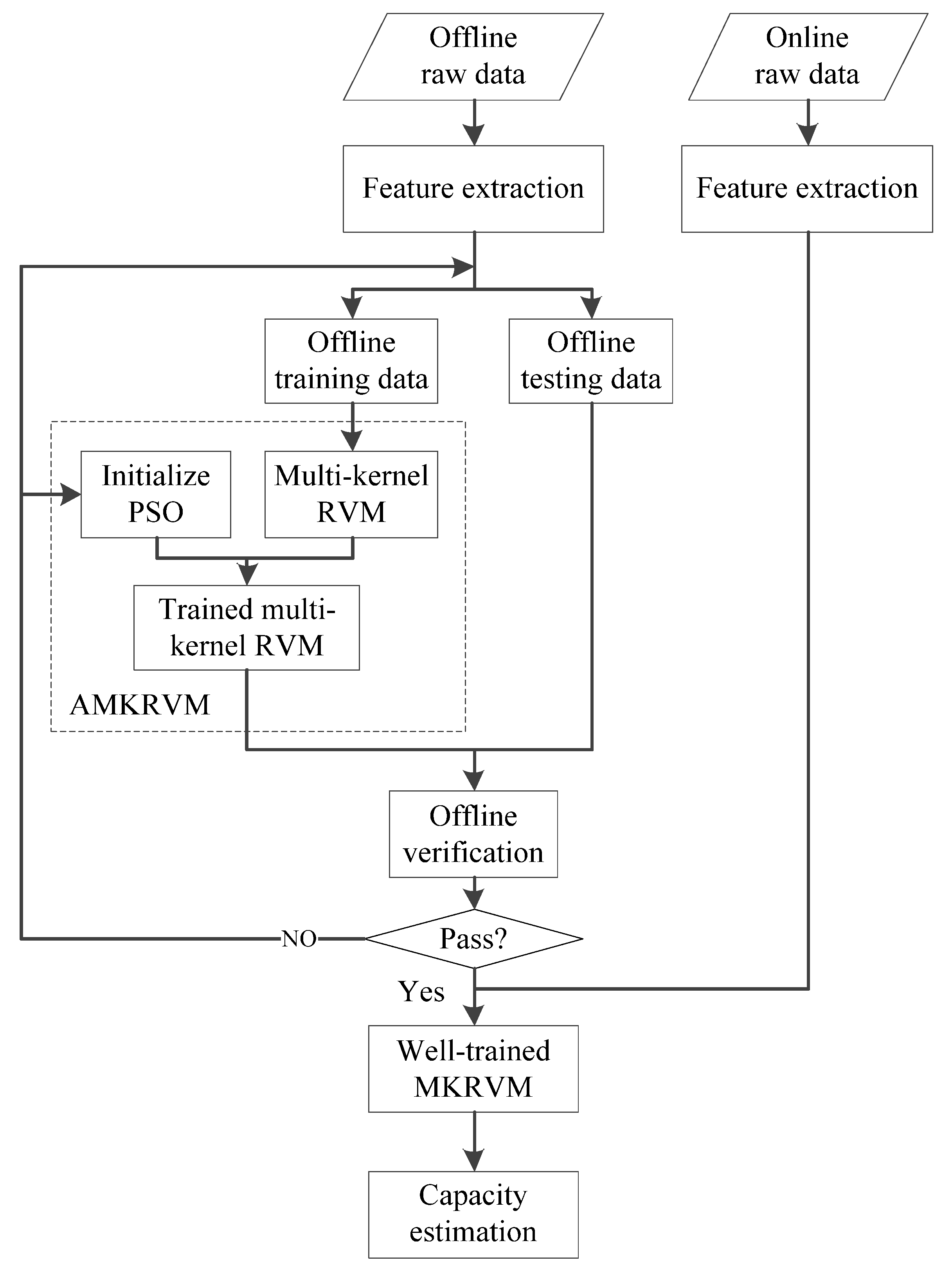
The overall procedure of the proposed method for online capacity estimation is shown in Figure 4. The procedure consists of two modules: offline and online stages.

Offline data are traditionally used only to determine unknown parameters in a specific model for online capacity estimation [21]. In this paper, a supervised learning process is proposed to utilize part of the offline data to ensure the generalizability of the model. In the proposed offline stage, the degradation features are extracted from the offline raw data. The processed offline data are then divided into two parts, one part for AMKRVM training and the other part for offline verification. Training data are used to determine the optimal combination of the kernel parameters in MKRVM via the APSO method. However, training is an MKRVM regression process. Training data can be utilized to measure regression accuracy, but not to test the generalizability of MKRVM. Even if the objective function in Equation (17) is adopted to avoid the over-fitting phenomenon to a great extent, the local optimization of the kernel parameters cannot be completely avoided. Prior to APSO implementation, several parameters that affect the APSO performance should be initialized. For example, the initial maximum iteration and particle size considerably influences the running time and convergence of the method, whereas the learning factors affect the search ability of APSO. Thus, we establish a supervised learning step in the offline stage. Part of the offline data is used to verify the generalizability of the trained MKRVM. According to the offline test results and a certain verification criterion, parameter settings in the APSO algorithm can be adjusted to achieve time saving and global optimum, and ensure the usability of MKRVM for online applications.

During the online stage, online data with well-trained and verified MKRVM are employed for online capacity estimation.

Figure 4. Overall procedure for capacity estimation.

Figure 4. Overall procedure for capacity estimation.

5. Experimental Results and Discussion

5.1. Data Sources

In the experiments presented in Section 2.1, the lithium-ion batteries used had the same specification and ambient temperature within batches. However, experimentation on different batteries was conducted at different discharge levels, and the discharge current varied among different batches. The data from three batches are utilized to verify the robustness and universality of the proposed model. Detailed information on the data sources is listed in Table 3. As the ambient temperature is the same within a batch, this parameter is not further considered in the model. AMKRVM is separately trained and tested based on each batch.

The total number of C-D cycles of batteries in the three batches was 168, 40 and 72, respectively. However, battery 18 only had 140 cycles. Furthermore, the third batch had three outliers in the raw data. For battery Nos. 45–48, the discharge steps were terminated too early after 20, 54, and 66 C-D cycles, at voltage levels of 3.45, 3.31 and 3.457 V, respectively. The corresponding capacity values were measured as zero by mistake. Thus, before using the data of the third batch, these outliers should be removed.

Table 3. Detailed information on data sources.

Batch	Battery No.	Ambient Temperature (°C)	Cutoff Voltage (V)	Discharge Current (A)
1st	5, 6, 7, 18	24	2.7, 2.5, 2.2, 2.5	2
2nd	29, 30, 31, 32	43	2.0, 2.2, 2.5, 2.7	4
3rd	45, 46, 47, 48	4	2.0, 2.2, 2.5, 2.7	1

Table 3. Detailed information on data sources.

Batch	Battery No.	Ambient Temperature (°C)	Cutoff Voltage (V)	Discharge Current (A)
1st	5, 6, 7, 18	24	2.7, 2.5, 2.2, 2.5	2
2nd	29, 30, 31, 32	43	2.0, 2.2, 2.5, 2.7	4
3rd	45, 46, 47, 48	4	2.0, 2.2, 2.5, 2.7	1

5.2. Battery Features and Analysis

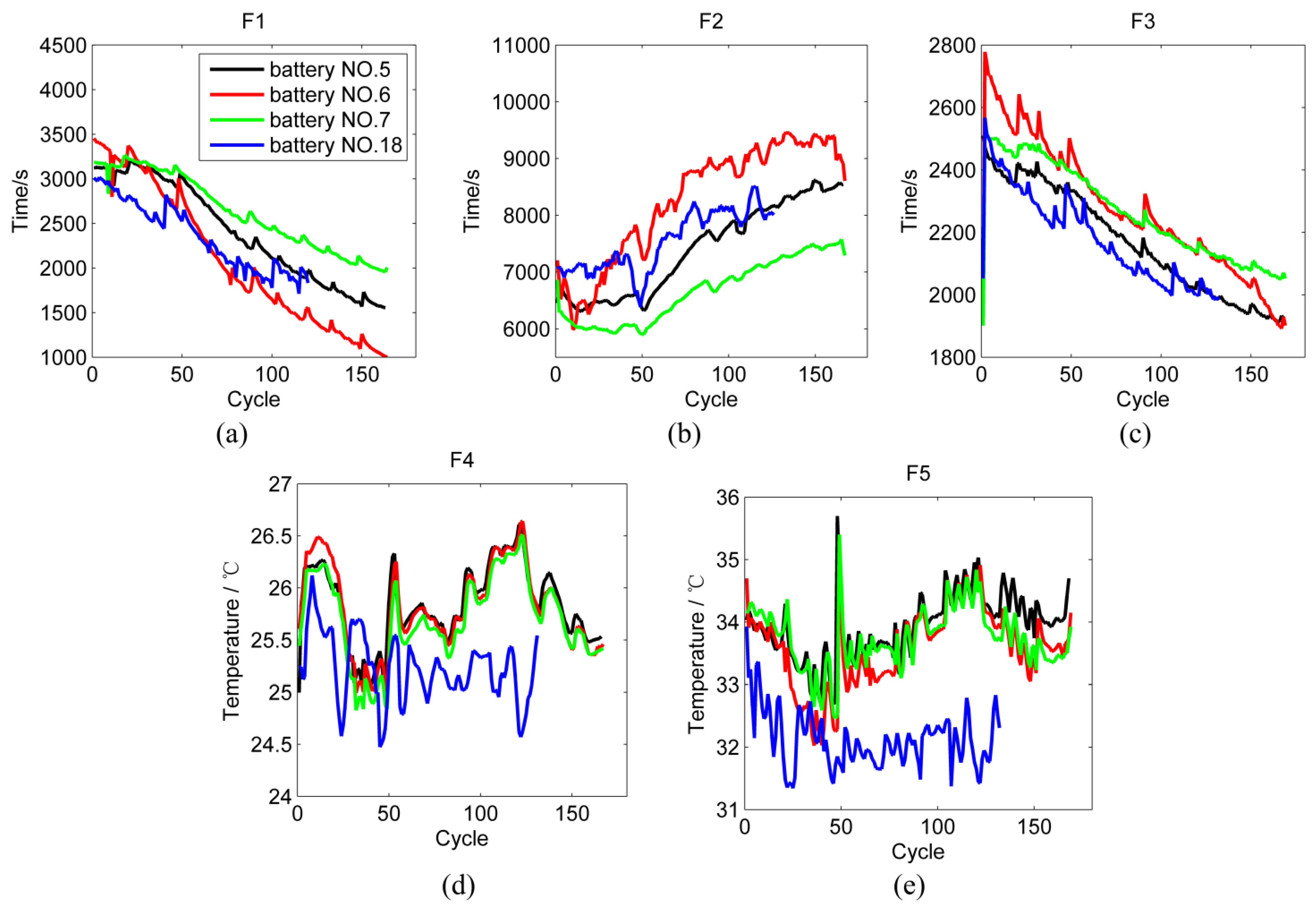
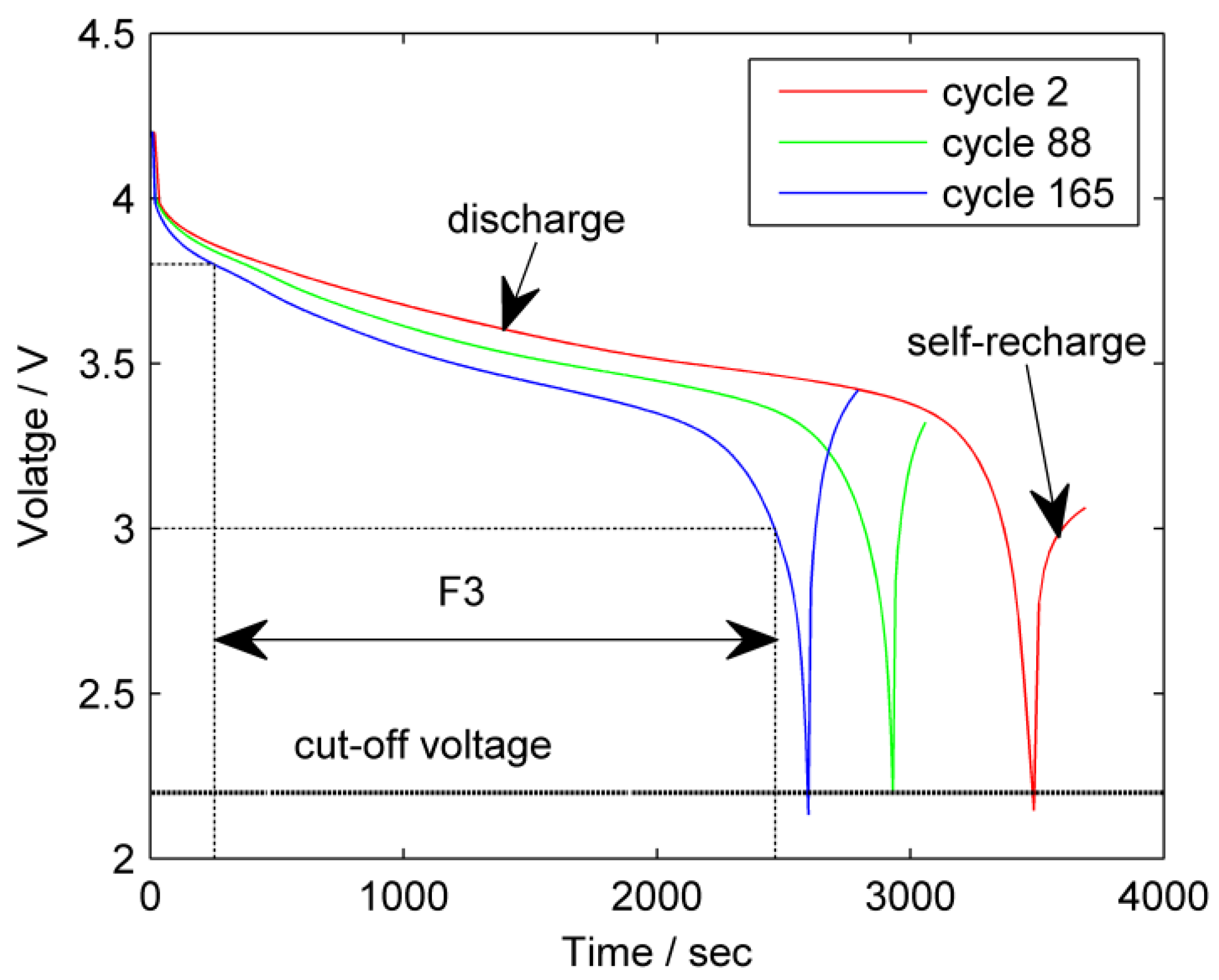
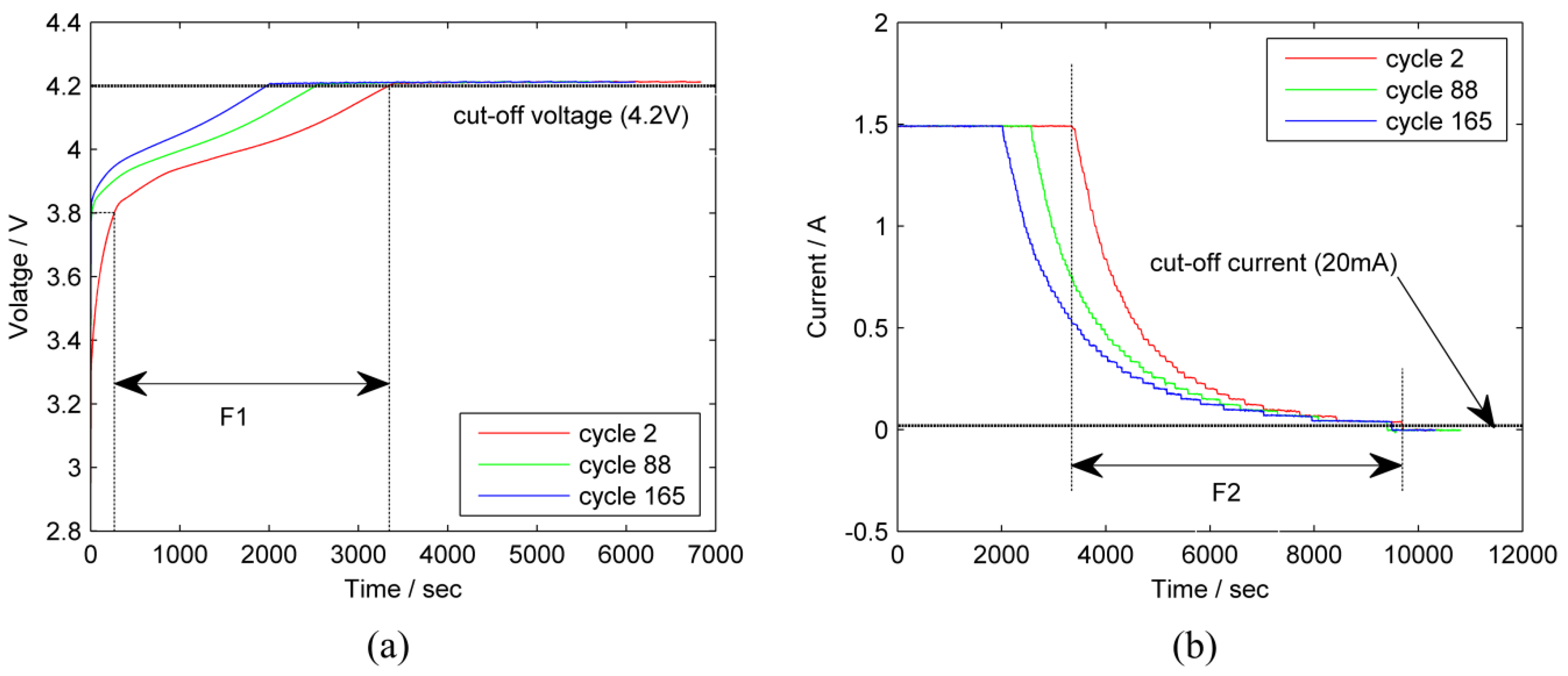
Considering the partial discharge during on-line operation, F₁ is set to be the time interval in which the charge voltage increases from 2.7 to 4.2 V, and F₃ is the time interval in which the discharge voltage decreases from 3.7 to 2.7 V. For example, the results of feature extraction of batteries in the first batch are given in Figure 5.

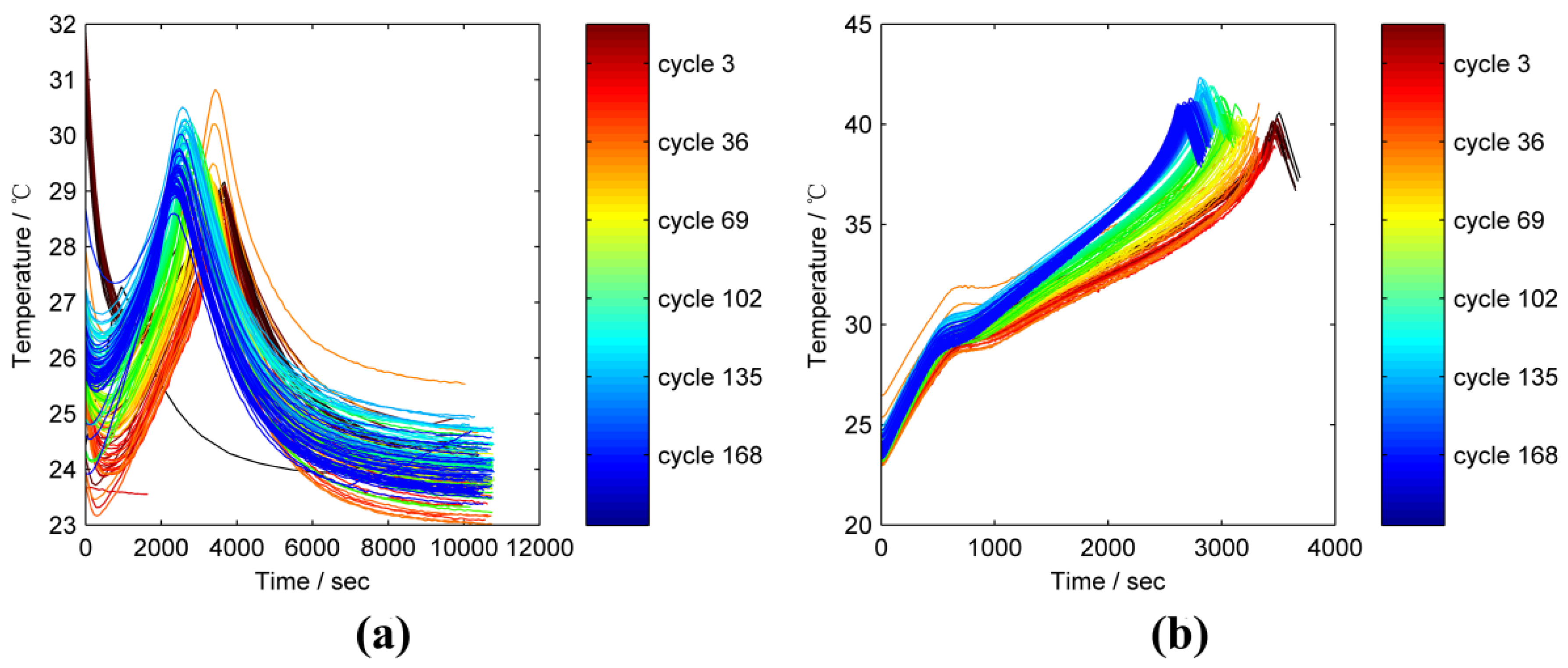
In Figure 5d,e, T_c and T_d change nonlinearly and non-monotonically over time. According to the heat-generation equation proposed by Bernard et al. [35]:

$$Q=\frac{I}{{Vol}_{total}}\left(V_{oc}-V-T\frac{d{V}_{oc}}{dT}\right)$$

(20)

where Q is the heat generated during battery operation; T is the temperature; $I$, Vol_total, V_oc, and V denote the current, total volume, open-circuit, and working voltage of the battery, respectively. According to Equation (20), the generated heat Q contrarily decreases with increasing temperature. Pals and Newman [36] proved that the heat-generation rate is higher for low temperatures than for high temperatures. Thus, the temperature of a battery does not keep rising during C-D cycles and must be considered because it influences the battery capacity.

Figure 5. The curves of the first five features of batteries in the first batch. (a) Feature F₁; (b) Feature F₂; (c) Feature F₃; (d) Feature F₄; (e) Feature F₅.

Figure 5. The curves of the first five features of batteries in the first batch. (a) Feature F₁; (b) Feature F₂; (c) Feature F₃; (d) Feature F₄; (e) Feature F₅.

5.3. Capacity Estimation Results and Discussion

In each batch, the first three batteries provide offline data, and the last one provides online data. During training and verification, all input features and output capacity are normalized to the interval [0, 1]. Estimation results are presented below.

5.3.1. Evaluation Criterion

Three evaluation criteria are used to measure the performance and accuracy of the proposed approach.

(1)

Root mean square error (RMSE) is a good measure of local accuracy, used to compare the estimation errors of the model:

$${\mathrm{\epsilon }}_{RMS}=\sqrt{\frac{1}{N_p}{{\displaystyle \sum }}_{i=1}^{N_p}{(C_i-{\widehat{C}}_i)}^2}$$

(21)

(2)

Mean relative error (MRE) compares how incorrect a quantity is from an estimated capacity considered to be true:

$${\mathrm{\epsilon }}_{MR}=\left(\frac{1}{N_p}{{\displaystyle \sum }}_{i=1}^{N_p}\left|\frac{C_i-{\widehat{C}}_i}{C_i}\right|\right)\times 100\%$$

(22)

(3)

Coefficient of determination (R²): indicates the fitness of data in a statistical model and gives information about the goodness of fit of a model. If the estimation is accurate, R² will be close to 1.

$$R^2=1-\frac{{{\displaystyle \sum }}_{i=1}^{N_p}{\left(C_i-{\widehat{C}}_i\right)}^2}{{{\displaystyle \sum }}_{i=1}^{N_p}{\left(C_i-{\overline{C}}_i\right)}^2}$$

(23)

where C_i is the actual capacity; ${\widehat{C}}_i$ is the estimated capacity; ${\overline{C}}_i$ is the mean value of the estimated capacity; and N_p is the sample size.

5.3.2. Offline Training and Verification

In each batch, the front half data of each battery is used to train AMKRVM, and the back half data are used for verification. In the verification step, the criterion can be established according to engineering requirement. In this case, AMKRVM is assumed well trained if over 90% real capacity values are covered by the 95% confidence intervals (CIs).

The optimal parameters of MKRVM determined by the APSO method are summarized in Table 4. The optimal values of the three parameters depend on a specific dataset and vary in different batches. Thus, determining the optimal parameters is significant. In the verification step, despite changes in the parameter settings of APSO, the variations in the optimization results are relatively small, showing the robustness of the optimization algorithm. However, through verification steps, the running time can be saved by changing the maximum number of iterations or particle size of APSO on the premise of convergence of the algorithm.

Table 4. The optimal parameters of the multi-kernel relevance vector machine (MKRVM).

Batch	Optimal Parameters
	r	s	ρ
1st	4.60	0.92	0.49
2nd	19.56	1.16	0.66
3rd	0.50	1.08	0.16

Table 4. The optimal parameters of the multi-kernel relevance vector machine (MKRVM).

Batch	Optimal Parameters
	r	s	ρ
1st	4.60	0.92	0.49
2nd	19.56	1.16	0.66
3rd	0.50	1.08	0.16

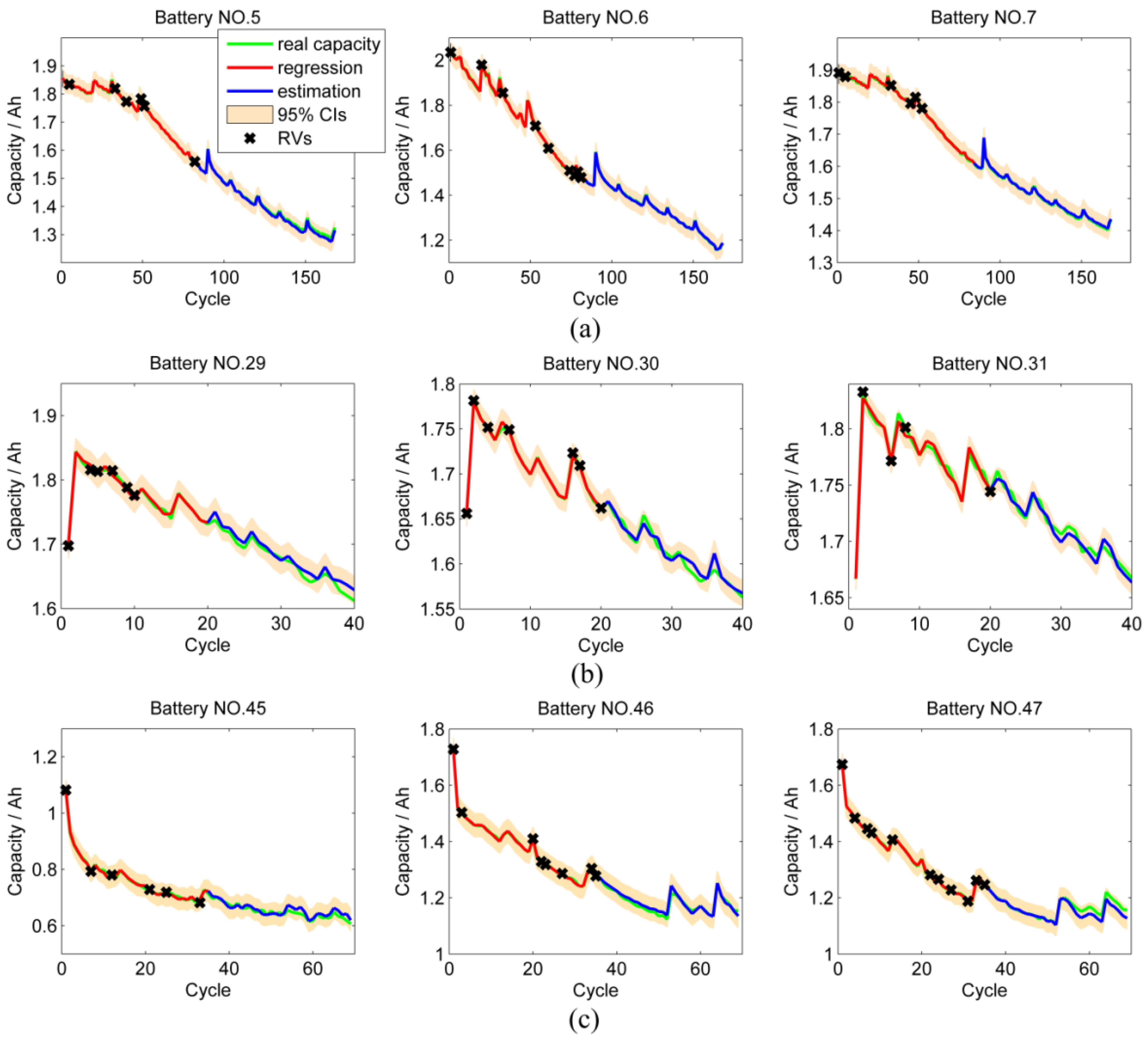
The regression and estimation results during offline training and verification of nine batteries are shown in Figure 6. Asterisks in Figure 6 represent relevance vectors (RVs), which form the sparse solution. The small number of RVs indicates the sparse property of MKRVM. Figure 6 also shows that most real capacity values lie within the 95% CIs. The degradation rates of battery capacity in distinct batches vary because of different ambient temperatures and discharge currents.

Table 5 summarizes the regression and estimation errors. Overall, in the three batches, the proposed model performs well in the regression and estimation process. Interestingly, in the first batch, some estimation errors are even less than regression errors, indicating the good generalizability of MKRVM. In the second batch, data size is relatively small, but values of RMSE and MRE are less than 0.01 and 1%, respectively; and even the smallest R² is more than 0.9. The results of the second batch demonstrate that the proposed approach can deal with a sparse dataset. In the third batch, regression errors are small, but the values of R² of the estimated capacity of batteries 45 and 47 are slightly far from 1. In Figure 6c, the back half data of batteries in the third batch are highly nonlinear and fluctuate. Cameron et al. [37] proved that negative or small R² values may occur when fitting nonlinear functions to the data because of the computational definition of R². Thus, small R² values in the third batch are rational. The values of RMSE and MRE in the estimation results in the third batch are also acceptable. In addition, as the 95% CIs can cover most of the real battery capacity, the performance of the proposed approach on the datasets of batteries in the third batch is considered satisfactory.

Figure 6. Regression and estimation results during the offline training and verification for the three batches of nine batteries. (a) Batteries 5–7; (b) batteries 29–31; (c) batteries 45–47.

Figure 6. Regression and estimation results during the offline training and verification for the three batches of nine batteries. (a) Batteries 5–7; (b) batteries 29–31; (c) batteries 45–47.

The offline verification process confirms the generalizability of the well-trained MKRVM. The experiment results demonstrate that the proposed AMKRVM can produce accurate and robust capacity estimation under various conditions.

Table 5. Regression and estimation errors during the offline training and verification process.

Batch	Battery	Regression Errors			Estimation Errors
		εRMS	ε MR (%)	R2	εRMS	εMR (%)	R2
1st	No. 5	0.0015	0.0592	0.9997	0.0072	0.4479	0.9817
	No. 6	0.0034	0.1362	0.9996	0.0033	0.2192	0.9972
	No. 7	0.0238	0.5609	0.9267	0.0055	0.2688	0.9869
2nd	No. 29	0.0046	0.2197	0.9835	0.0090	0.4608	0.9335
	No. 30	0.0020	0.0693	0.9966	0.0070	0.3466	0.9442
	No. 31	0.0043	0.1996	0.9842	0.0058	0.3309	0.9481
3rd	No. 45	0.0058	0.6436	0.9945	0.0116	1.4982	0.7446
	No. 46	0.0030	0.1784	0.9990	0.0096	0.6287	0.9316
	No. 47	0.0024	0.1465	0.9995	0.0149	0.9254	0.7613

Table 5. Regression and estimation errors during the offline training and verification process.

Batch	Battery	Regression Errors			Estimation Errors
		εRMS	ε MR (%)	R2	εRMS	εMR (%)	R2
1st	No. 5	0.0015	0.0592	0.9997	0.0072	0.4479	0.9817
	No. 6	0.0034	0.1362	0.9996	0.0033	0.2192	0.9972
	No. 7	0.0238	0.5609	0.9267	0.0055	0.2688	0.9869
2nd	No. 29	0.0046	0.2197	0.9835	0.0090	0.4608	0.9335
	No. 30	0.0020	0.0693	0.9966	0.0070	0.3466	0.9442
	No. 31	0.0043	0.1996	0.9842	0.0058	0.3309	0.9481
3rd	No. 45	0.0058	0.6436	0.9945	0.0116	1.4982	0.7446
	No. 46	0.0030	0.1784	0.9990	0.0096	0.6287	0.9316
	No. 47	0.0024	0.1465	0.9995	0.0149	0.9254	0.7613

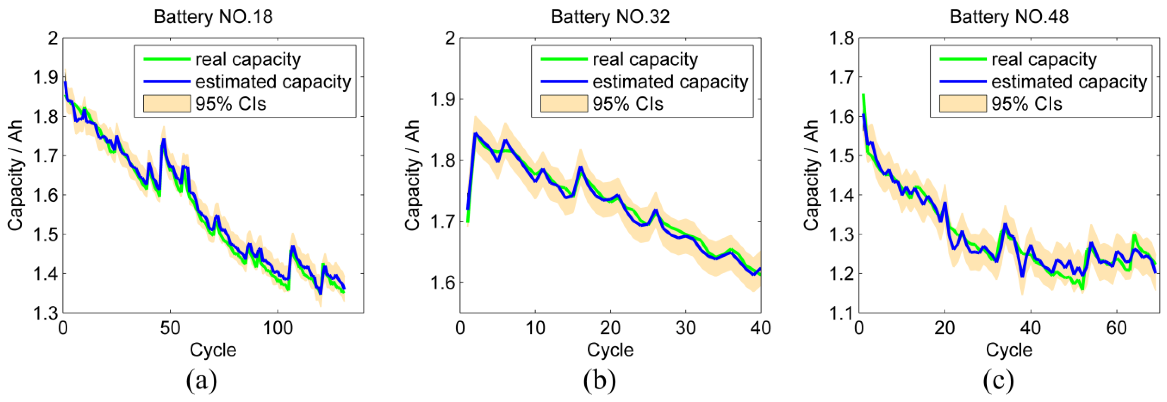
5.3.3. Online Estimation

The well-trained MKRVM is utilized to estimate the capacity of the fourth battery in each batch (Nos.18, 32 and 48). After offline verification, the well-trained MKRVM do not need to be trained again using the data of the online batteries. The estimation results obtained using parameters listed in Table 4 are summarized in Figure 7, and Table 6 shows the estimation errors. The 95% CIs can cover most of the real capacity values. Although the degradation data of online batteries is not utilized to estimate parameters in MKRVM, the method still performs well. The online estimation results verify the accuracy and effectiveness of the proposed approach.

Figure 7. Online capacity estimation results: (a) Battery 18; (b) Battery 32; (c) Battery 48.

Figure 7. Online capacity estimation results: (a) Battery 18; (b) Battery 32; (c) Battery 48.

Table 6. Estimation errors of the online estimated capacity.

Battery	Estimation Errors
	εRMS	εMR (%)	R2
No. 18	0.0155	0.8032	0.9898
No. 32	0.0077	0.3281	0.9870
No. 48	0.0119	0.5516	0.9508

Table 6. Estimation errors of the online estimated capacity.

Battery	Estimation Errors
	εRMS	εMR (%)	R2
No. 18	0.0155	0.8032	0.9898
No. 32	0.0077	0.3281	0.9870
No. 48	0.0119	0.5516	0.9508

5.4. Method Validation and Comparison

To verify the accuracy of the proposed approach, we conducted the first comparison study to determine the estimation errors of two other adaptive RVMs with a single kernel. The first model for comparison is an RVM with RBF kernel (M₁), and the second RVM only uses the polynomial kernel (M₂).

To utilize the dataset, a cross-validation (C-V) process is employed to assess the estimation performance of each model. In C-V, the original data are divided into two parts: one for training and the other part for testing. In each batch, M batteries are randomly selected as the training data and the remaining (4-M) batteries are used for testing. In each batch, the C-V process is repeated k = $C_4^{\mathrm{M}}$ times, with each of the four batteries used exactly $C_3^{\mathrm{M}-1}$ times as the validation data. Total C-V RMSE is computed as

$${\mathrm{\epsilon }}_{CV}=\sqrt{\frac{1}{U}{\displaystyle \sum }_{i=1}^k{\displaystyle \sum }_{x_n\in X_{test}^{\left(i\right)}}{\left(t_n-y_{X_{train}^{\left(i\right)}}\left(x_n\right)\right)}^2}$$

(24)

where $X_{test}^{\left(i\right)}$ and $X_{train}^{\left(i\right)}$ are the test and the training datasets in $i$th C-V process, respectively; $y_{X_{train}^{\left(i\right)}}$ denotes the AMKRVM model built with the test subset $X_{test}^{\left(i\right)}$; t_n is the actual response of the input $x_n\in X_{test}^{\left(i\right)}$; and $U$ is the total number of test data points for the $k$ C-V processes.

The comparison results are summarized in Table 7. The values of C-V RMSE of the AMKRVM are smaller than that of the two single-kernel models, which shows that the multi-kernel function enables the RVM to be more accurate and general than the single kernel. In online applications, the degradation data of the on-line battery are not used to train RVM, and generalizability plays a significant role in estimation. The results illustrate that the proposed AMKRVM approach has better performance in online applications than the other single-kernel RVMs under different conditions.

Table 7. Comparison results of C-V RMSEs of three models.

Batch	M	C-V RMSE
		EMKRVM	M1	M2
1st	3	0.0342	0.0573	0.0794
	2	0.0496	0.0767	0.0927
	1	0.0557	0.0975	0.1096
2nd	3	0.0107	0.0323	0.0779
	2	0.0155	0.0423	0.0878
	1	0.0148	0.0290	0.1001
3rd	3	0.0303	0.3047	0.3008
	2	0.0307	0.3491	0.3180
	1	0.0536	0.3522	0.4414

Table 7. Comparison results of C-V RMSEs of three models.

Batch	M	C-V RMSE
		EMKRVM	M1	M2
1st	3	0.0342	0.0573	0.0794
	2	0.0496	0.0767	0.0927
	1	0.0557	0.0975	0.1096
2nd	3	0.0107	0.0323	0.0779
	2	0.0155	0.0423	0.0878
	1	0.0148	0.0290	0.1001
3rd	3	0.0303	0.3047	0.3008
	2	0.0307	0.3491	0.3180
	1	0.0536	0.3522	0.4414

Additionally, C-V RMSEs of the proposed model under different training data size illustrate that more accurate estimated capacity can be obtained with more training data used. An opposite result occurs in the second batch when M decreases from 2 to 1. However, in Table 7, the increase in C-V RMSEs in the second batch during C-V processes is nearly negligible. The MKRVM performance on the second batch is stable. Similar conclusions can be drawn from Table 5. Thus, the aforementioned opposite result may be due to normal experimental errors. Overall, the C-V results validate the accuracy of the proposed model.

The second experiment compares the running time of the proposed AMKRVM with that of MKRVM that uses traditional PSO to search for optimal parameters. The results show that the iterative numbers of APSO (around 200 iterations) are less than that of the latter approach (around 340 iterations), thereby confirming the efficiency of the proposed method.

6. Conclusions

This paper proposes an ensemble and data-driven approach for online capacity estimation of lithium-ion batteries. First, six features are extracted from cyclic charge/discharge cycles and used as health indicators for a battery. An adaptive method based on MKRVM and APSO algorithm is then employed to regress and estimate the capacity. To ensure the robustness of the model for on-line application, we utilized offline data for training MKRVM and verifying method generalizability. Finally, cross-validation is performed in model comparison to validate the accuracy of the proposed model.

Experimental results demonstrate that the proposed approach has satisfactory performance under different conditions. AMKRVM can be used to automatically and effectively determine optimal parameter settings under distinct circumstances. The novel offline supervised learning step ensures the efficiency and robustness of the estimation. In model comparison, the cross-validation results show the validity of our model. Compared with single-kernel RVMs, the novel AMKRVM produces more accurate and robust estimation results. Besides, the C-V results indicate that estimation accuracy increases as more training data are used because of the relatively good coherence of the sample data. Finally, it shows that parameter optimization through APSO is also more efficient. The results verify that the proposed method is promising for online battery prognostics.

However, the AMKRVM training is limited in the same patch data because ambient temperature is not included as a variable in the model. The optimal parameters of MKRVM differ under varied ambient temperatures. As the influence of the ambient temperature on capacity degradation is highly demonstrated, further research must be performed to explore the effects of this parameter.