
A Multi Time Scale Wind Power Forecasting Model of a Chaotic Echo State Network Based on a Hybrid Algorithm of Particle Swarm Optimization and Tabu Search

Abstract
:1. Introduction
- (1)
- Firstly, the phase space reconstruction of chaotic time series is used to reduce the impact of the uncertainty of the original data;
- (2)
- Secondly, the ESN is introduced for prediction. As a new dynamic recurrent neural network, ESN has a unique simple training method and high precision training results. The introduction of reserve pool has overcome the problems of slow convergence and local minimum, which can bring about higher accuracy;
- (3)
- Considering the characteristics of the tabu search and particle swarm algorithm, the diversity principles of the tabu search algorithm are introduced into the mechanisms of “group share” and “random search” of particle swarm to make the search process have memory. The combination of the two algorithms provides complementary advantages to improve the prediction accuracy;
- (4)
- Considering the multitime scales of minutes, hours and days simultaneously, wind power predictions are carried out. Meanwhile, the seasonal factors are integrated into the model to analyze the characteristics of wind power, and the robustness and generalization ability of the proposed method is verified.
2. Chaotic Echo State Network (ESN)
2.1. Chaos Identification and Phase Space Reconstruction
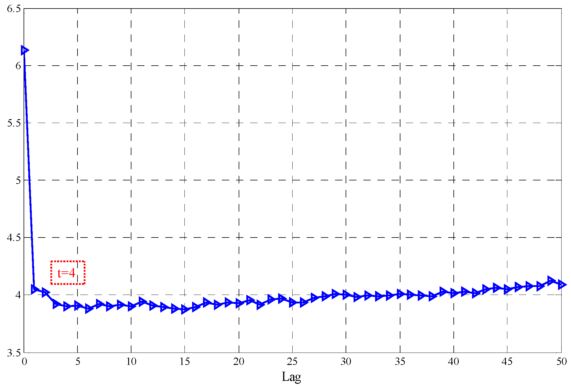
2.1.1. Mutual Information Method to Determine the Delay Time
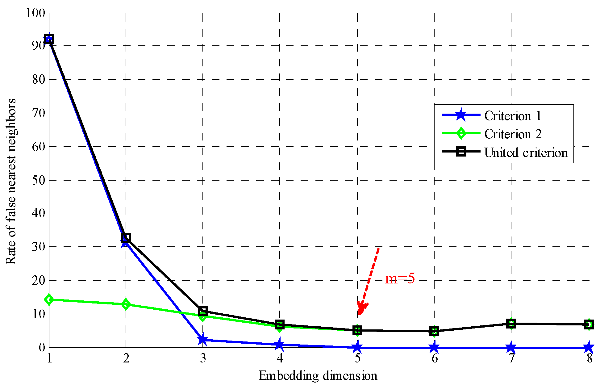
2.1.2. False Nearest Neighbors Method (FNN) to Determine the Embedding Dimension
2.1.3. The Maximum lyapunov Exponent for Chaotic Recognition
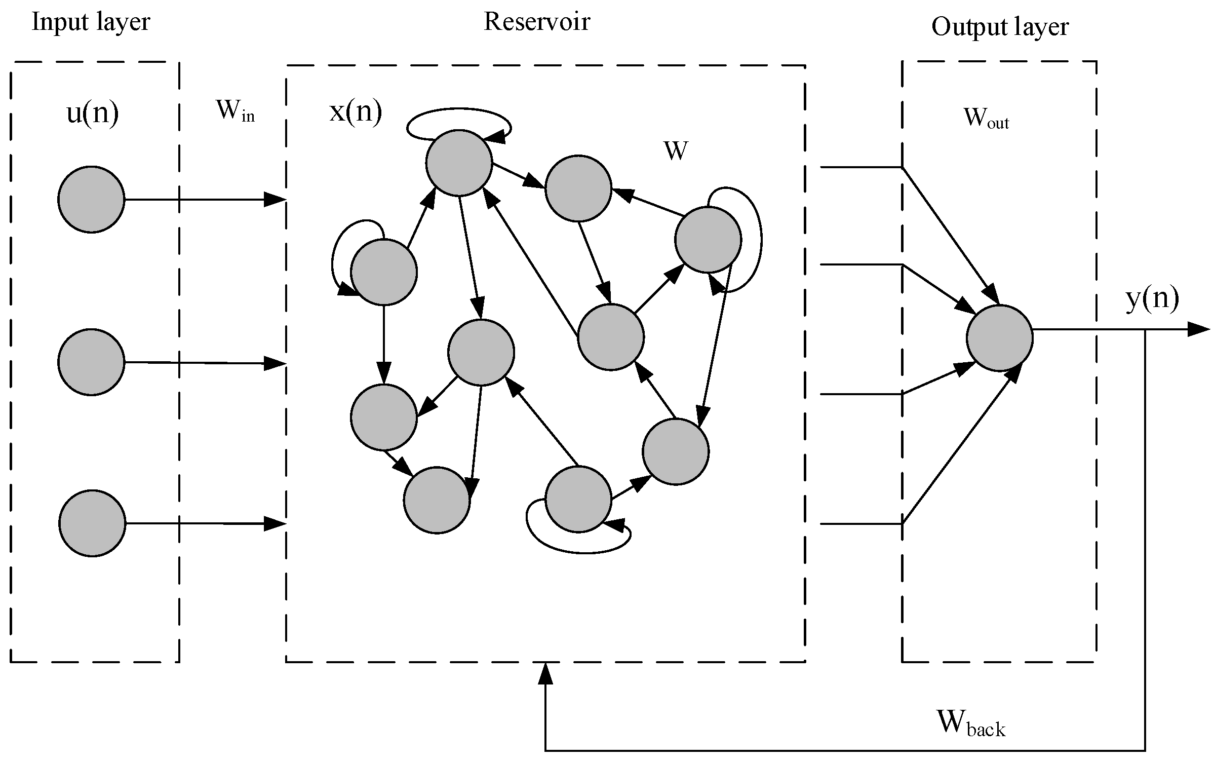
2.2. ESN
- (1)
- Initialize the ESN. The weight matrixes and are generated randomly, elements of them are initialized to random numbers obeying [0, 1] uniform distribution, and will not change once produced. The state vector is set to zero;
- (2)
- Update the state vector of ESN reservoir. According to the formula Equation (4), calculate the new reservoir state vector with the given input vector and state connection vector ;
- (3)
- Calculate the output weight matrix . Select all state connection vectors and desired output vectors after the time point , then train the weight matrix according to the following formulas:
- (4)
- After completing the training of output weight matrix , set all the input vectors after time point as the test input vectors and take them into the Equation (5) to get the predicted output vector .
2.3. The Prediction Steps of Chaotic ESN
- (1)
- (2)
- Learning period. Select a certain length time series, and train the network using the matrix X as input and the vector Y as output. By adopting the output of the before process, compare the result with the target model. If there is any error, start the back-propagation process immediately, and correct the network weights in order to reduce error.
- (3)
- Forecasting period. The input of ESN is set to be , and then the output will be the actual prediction value of the sequence. The predicted value should be used in the iteration prediction, as the network input of a new round.
3. Theoretical Introduction of Optimization Algorithm
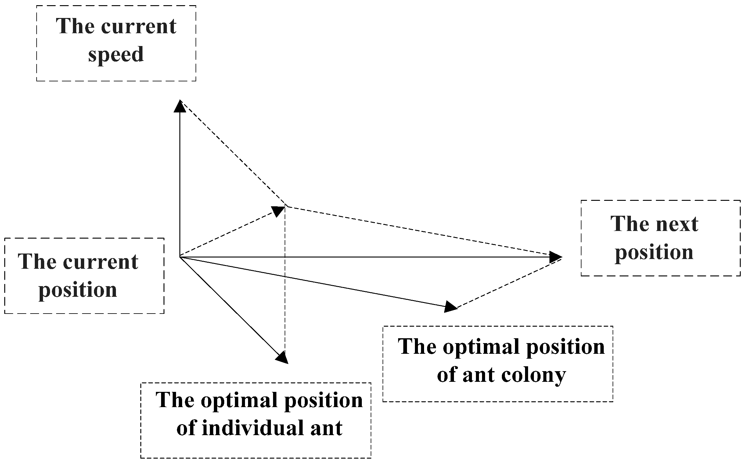
3.1. Basic Theory of Particle Swarm Optimization

3.2. Tabu Search
- (1)
- Encoder mode: the initial solution of the TS can be randomly generated. It can also be readily obtained by means of heuristics based on the properties of the problem at hand;
- (2)
- The choice of candidate solutions: the number of candidate solutions should be firstly determined followed by the choice of the optimal candidate solution. In principle, all neighborhood solutions of the current solution should be executed. However, when the scale of a problem is large, there will be a great number of neighborhood solutions. Considering the efficiency of neighborhood search, it is better to merely select subsets of the neighborhood. As for the selection of best candidate solution, the general approach is to choose the best one that meets the principle of contempt or non-taboo in the set of candidate solutions;
- (3)
- Tabu table and its length: tabu table usually adopts a FIFO queue and its length can be fixed or change adaptively;
- (4)
- Contempt principles: it often uses simple contempt principles that if a solution is better than the optimum, its tabu properties are ignored. The solution are selected as the current solution;
- (5)
- Termination condition: the common condition is the maximum number of functions or the maximum continuous iteration number when the best solution can sustain.
3.3. Hybrid Algorithm Based on Particle Swarm Algorithm and Tabu Search
4. Chaotic ESN Optimized by Particle Swarm and Tabu Search
- (1)
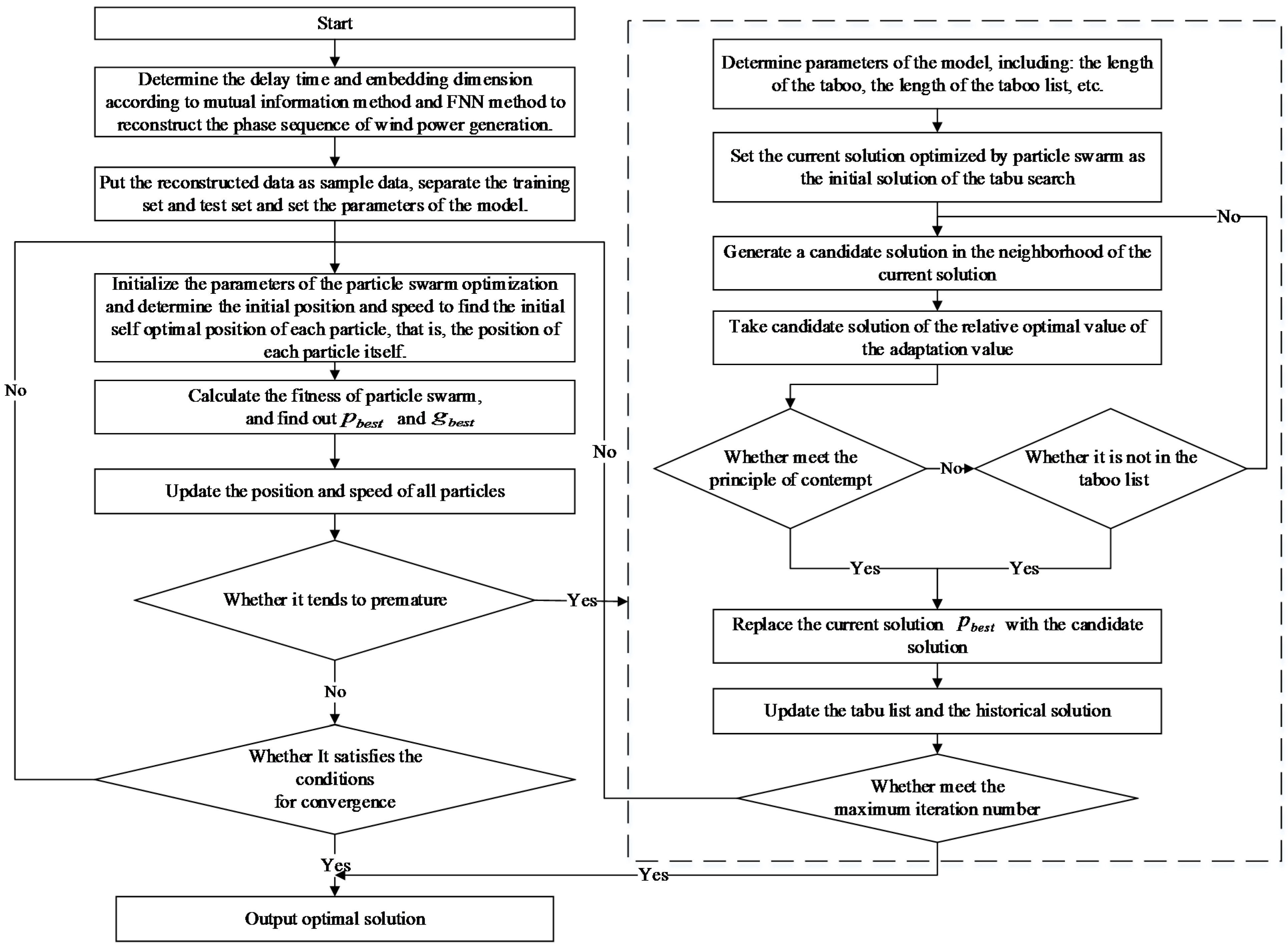
- Determine the delay time and embedding dimension m according to the mutual information method and FNN method to reconstruct the phase sequence of wind power generation;
- (2)
- Use the reconstructed data as sample data, separate the training set and test set and set the parameters of the model, including: particle swarm size M, iteration number, tabu search length, etc.;
- (3)
- Initialize the parameters of the particle swarm optimization and determine the initial position and speed to find the initial self-optimal position of each particle, that is, the position of each particle itself;
- (4)
- Calculate the fitness of particle swarm, and find out and ;
- (5)
- Update the position and speed of all particles according to Equations (13) and (14);
- (6)
- According to Equation (15), judge that whether the particle tends to premature. If yes, then go to the next step of tabu search; otherwise, determine whether the particle swarm optimization meet the convergence condition, if yes, then output results, otherwise, go to Step (3);
- (7)
- Set the current solution optimized by particle swarm as the initial solution of the tabu search, use the neighborhood function of the current global extremum to produce a number of neighborhood values, and select some candidate solutions with the highest fitness;
- (8)
- Judge each candidate using the contempt criterion, if satisfactory, replace the current solution with the candidate solution and update the tabu list and optimal solution, then go to the Step (6), otherwise, proceed to the next step;
- (9)
- Judge whether the candidate solution is in the tabu list, select the best state instead of the current solution, find the corresponding tabu object to replace the taboo object which firstly entered the tabu table;
- (10)
- Judge whether meet the maximum iteration number, if yes, then output optimal solution, otherwise, go to Step (3).
5. Empirical Analysis
5.1. Multi Time Scale Forecasting of Short-term Wind Power Generation without Considering Seasonal Factors
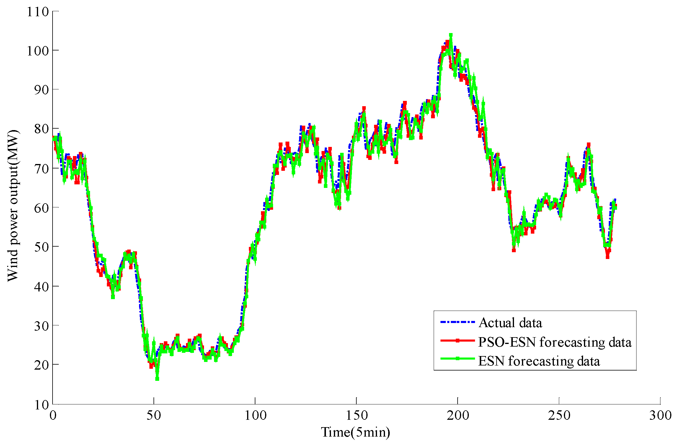
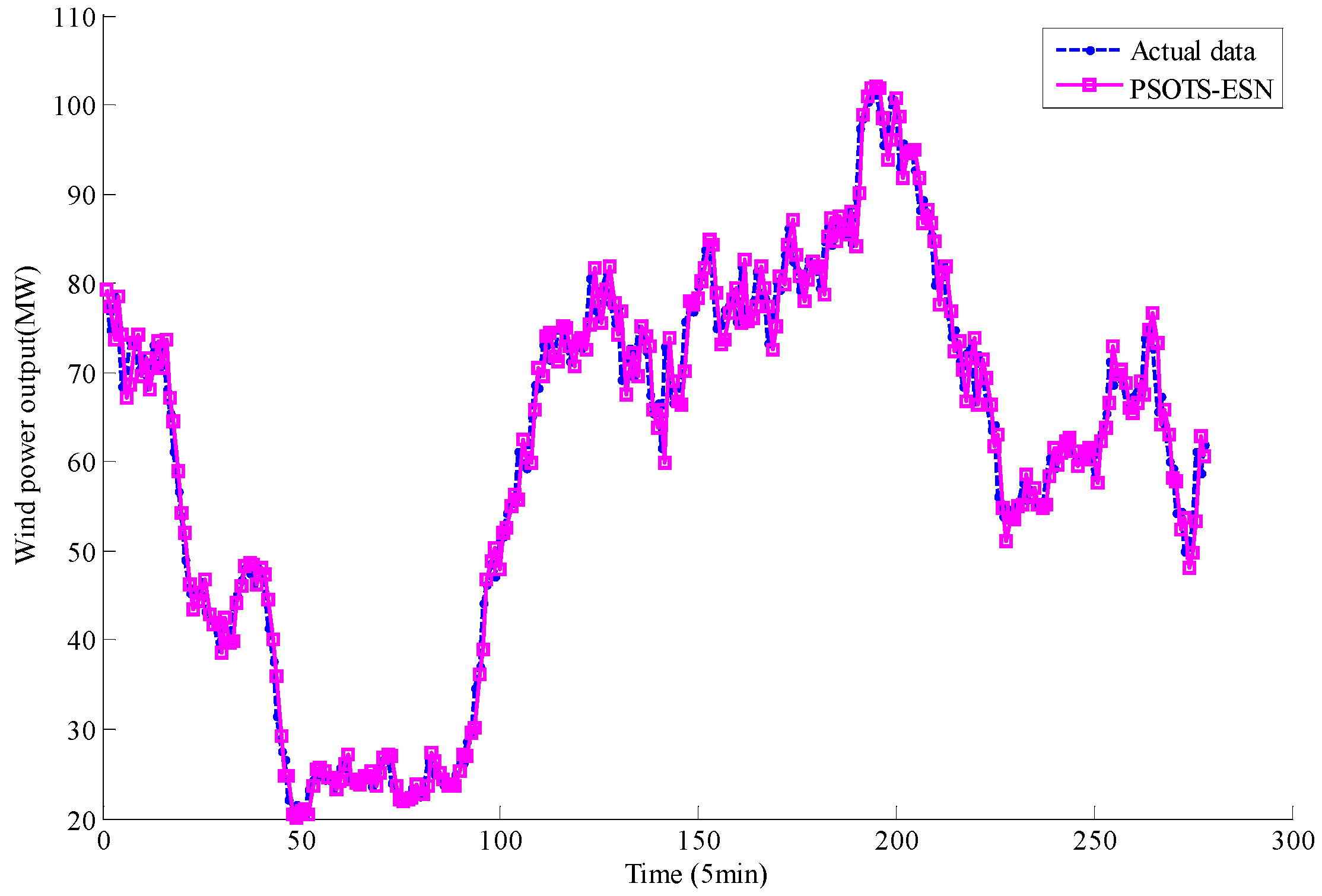
5.1.1. Ultrashort-Term Wind Power Generation Based on the Time Scale of 5 Min


| Algorithm | MAPE (%) | MAE (MW) | RMSE (MW) | Computational time (s) |
|---|---|---|---|---|
| PSOTS-ESN | 3.97 | 8.82 | 2.97 | 144 |
| PSO-ESN | 5.51 | 12.7 | 3.49 | 152 |
| ESN | 7.79 | 14.43 | 3.75 | 155 |
| BP | 8.6 | 15.8 | 4.8 | 201 |


- (a)
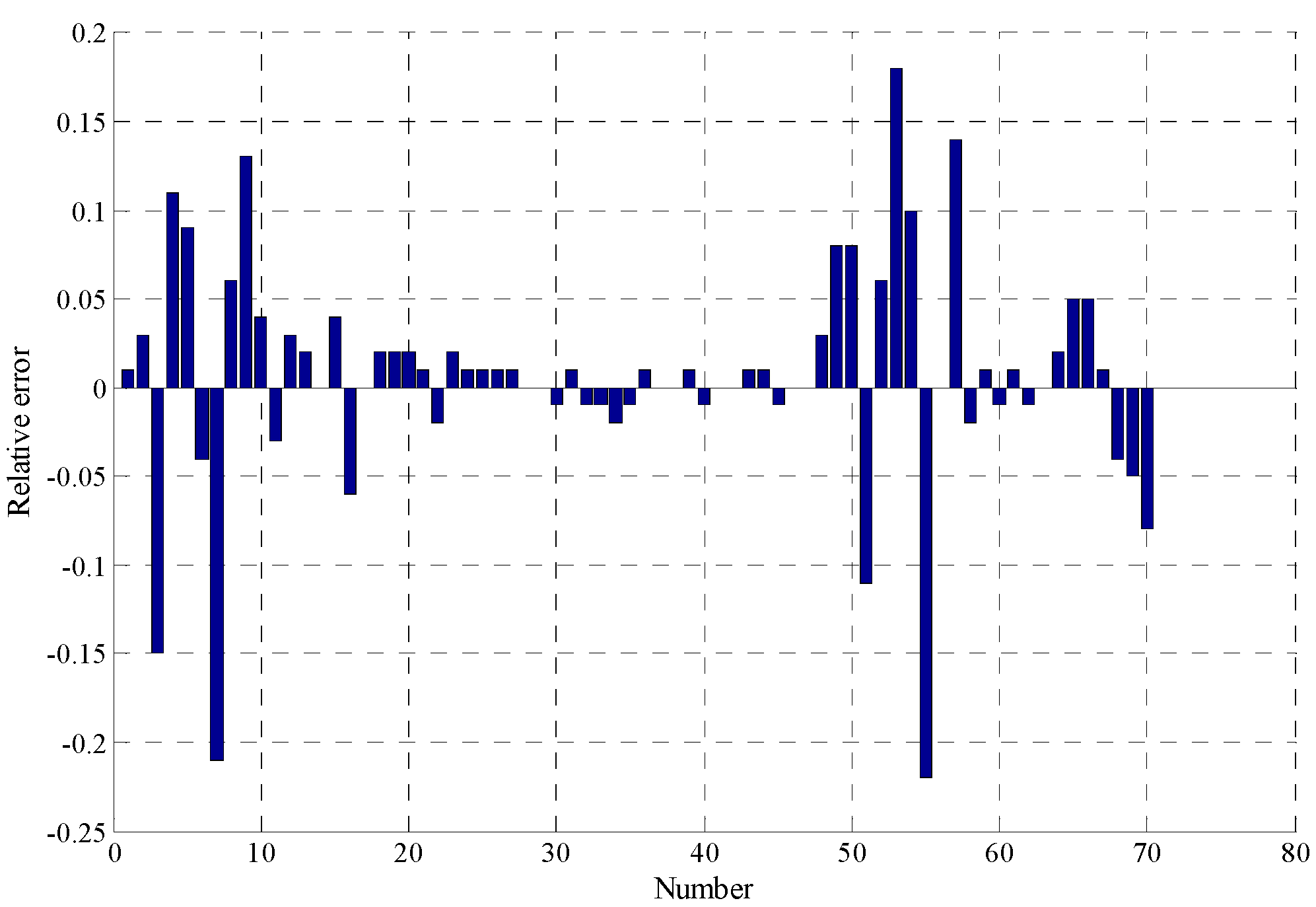
- The result of Figure 8 and Figure 9 and Table 1 denote that the proposed PSOTS-ESN model in this paper has more obvious advantages than the PSO-ESN model. The error metrics and computation time of the PSOTS-ESN are all less than those of the PSO-ESN model. The main reason is the fact that the hybrid optimization algorithm makes up for the defects of any single algorithm and chaotic time reconstruction can eliminate the chaos of the original data without regularity which improves the accuracy and the generalization ability of the model and makes for a better prediction effect.
- (b)
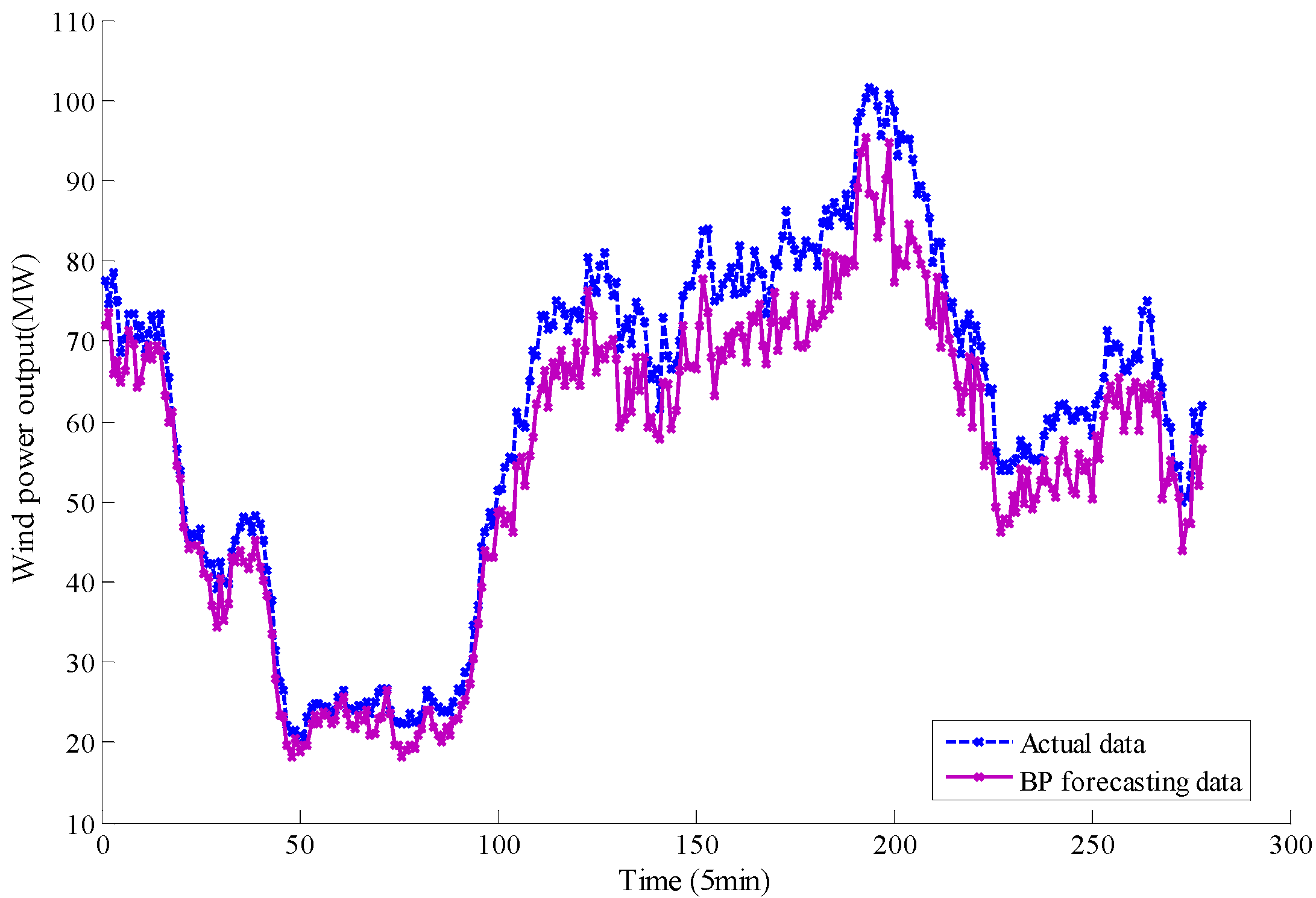
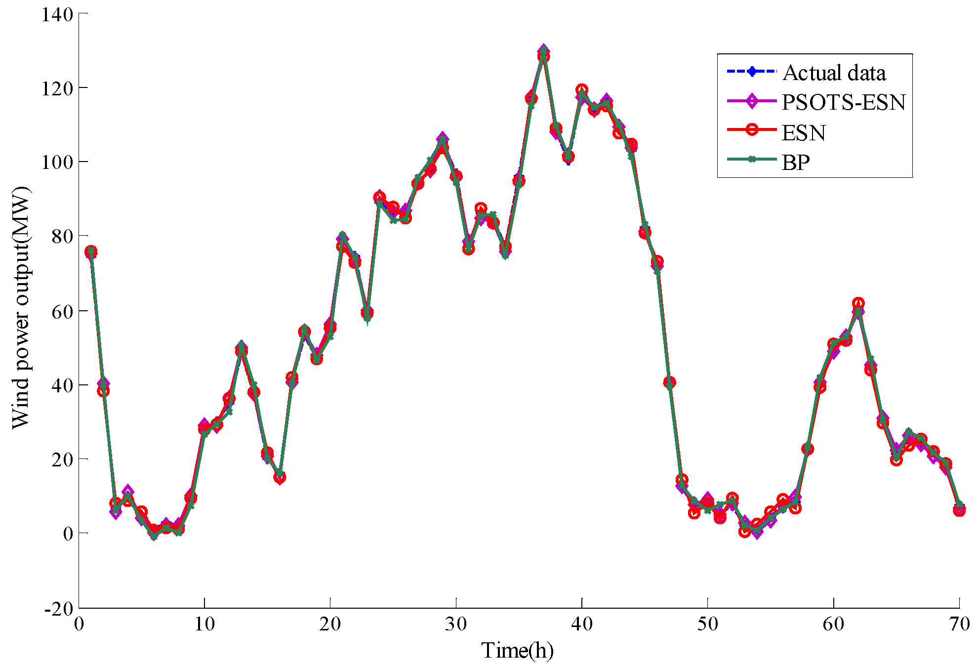
- Comparing Figure 8, Figure 9 and Figure 10, we can find that the forecasting precision of the combined model is higher than that of the single model. As the combination forecasting model can realize the complementary advantages of different algorithms to improve the accuracy of the algorithm, the prediction of a single model has a large limitation.
- (c)
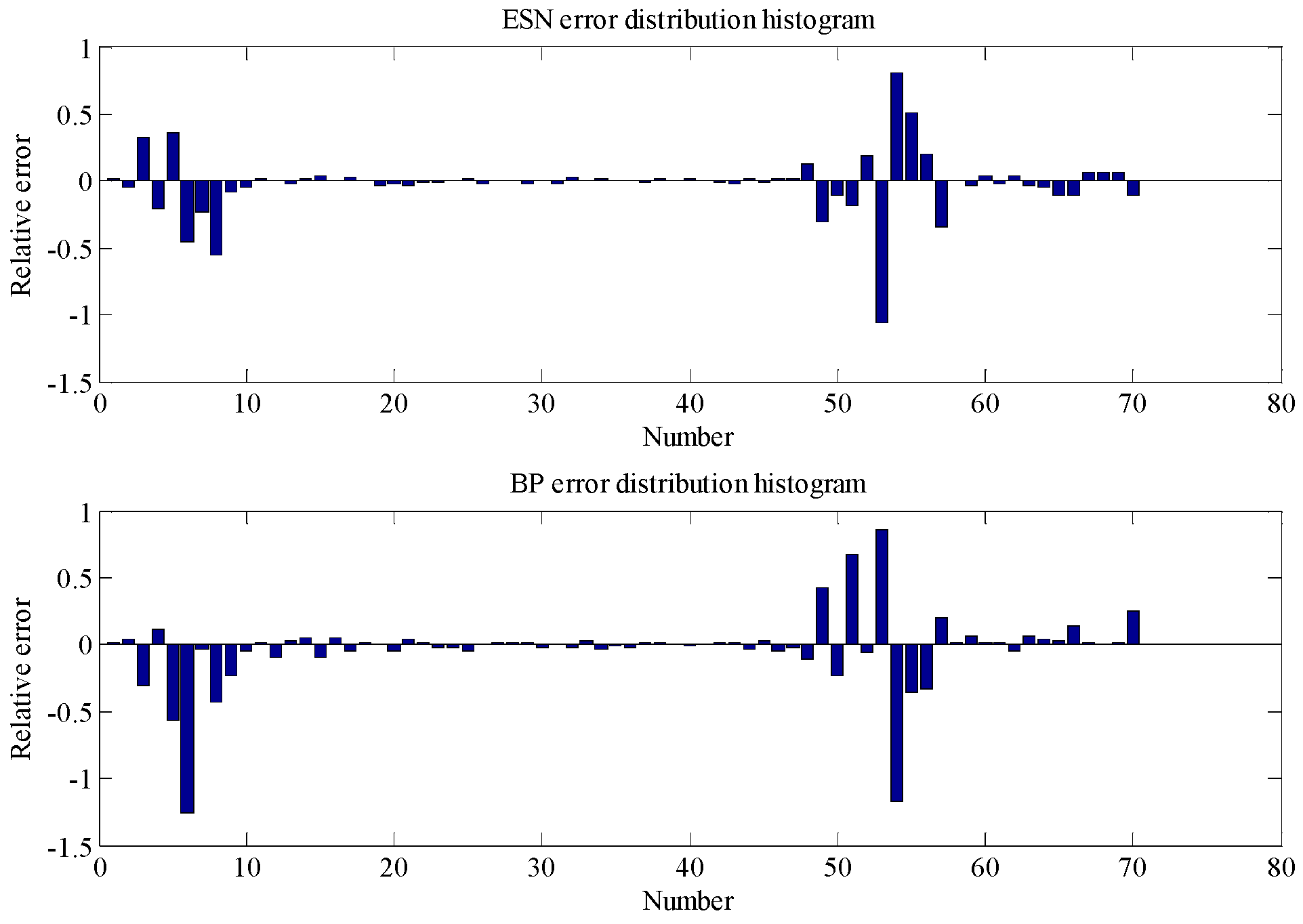
- From Figure 9 and Figure 10 and Table 1, we can find that the forecasting precision of the standard ESN is higher than that of the BP neural network. The conclusion can be drawn as follows: for the forecasting of non-stationary time series, the processing power of ESN is better than that of BP, and the prediction accuracy is higher.
5.1.2. Short-Term Wind Power Generation Based on the Time Scale of 1 H


| Algorithm | MAPE (%) | MAE (MW) | RMSE (MW) |
|---|---|---|---|
| PSOTS-ESN | 5.9012 | 0.68 | 0.63081 |
| ESN | 9.7283 | 1.03 | 1.3733 |
| BP | 9.0579 | 1.15 | 1.8571 |
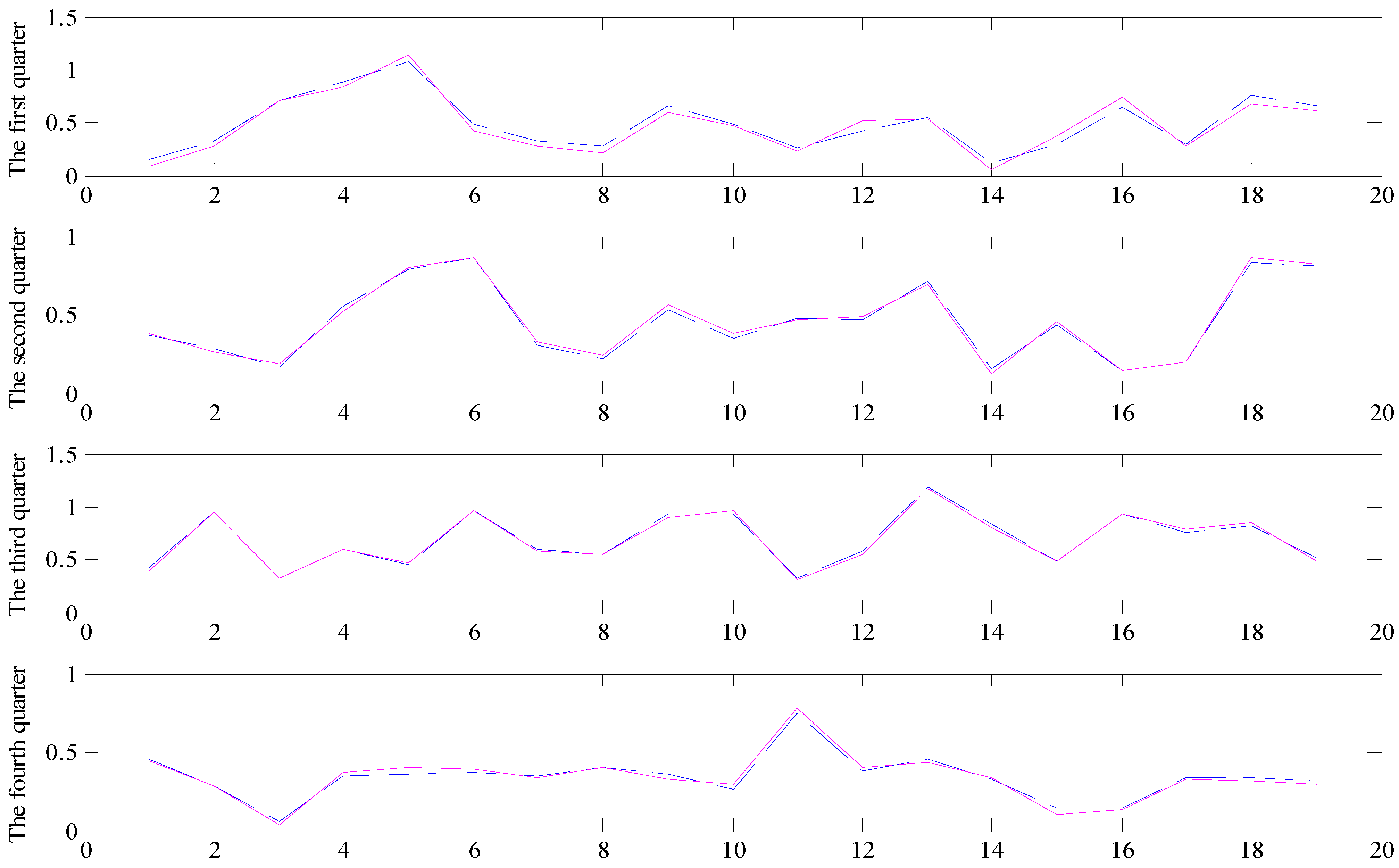
5.2. Multi Time Scale Forecasting of Short-term Wind Power Generation considering Seasonal Factors

| Error | First quarter | Second quarter | Third quarter | ||||||
| PSOTS-ESN | ESN | BP | PSOTS-ESN | ESN | BP | PSOTS-ESN | ESN | BP | |
| MAPE | 3.231 | 4.5 | 5.98 | 8.2 | 10.3 | 12.6 | 8.8 | 9.2 | 10.7 |
| RMSE | 6 × 10⁻⁴ | 1 × 10⁻³ | 2 × 10⁻³ | 5.5 × 10⁻⁴ | 1 × 10⁻³ | 2 × 10⁻³ | 8 × 10⁻⁴ | 3 × 10⁻³ | 2 × 10⁻² |
| MAE | 2 × 10⁻² | 3 × 10⁻² | 3 × 10⁻² | 2 × 10⁻² | 2 × 10⁻² | 3 × 10⁻² | 5 × 10⁻² | 4 × 10⁻² | 5 × 10⁻² |
| Error | Fourth quarter | Non-seasonal factor forecasting | - | - | - | ||||
| PSOTS-ESN | ESN | BP | PSOTS-ESN | ESN | BP | - | - | - | |
| MAPE | 5.52 | 9.6 | 13.5 | 11.79 | 13.5 | 18.4 | - | - | - |
| RMSE | 5 × 10⁻⁴ | 1 × 10⁻² | 2 × 10⁻³ | 3 × 10⁻² | 0.4 | 0.8 | - | - | - |
| MAE | 1 × 10⁻² | 2 × 10⁻² | 4 × 10⁻² | 0.19 | 0.34 | 0.61 | - | - | - |
6. Conclusions
Acknowledgments
Author Contributions
Conflicts of Interest
References
- Wang, J.Z.; Hu, J.M.; Ma, K.L. A self-adaptive hybrid approach for wind speed forecasting. Renew. Energy 2015, 78, 374–385. [Google Scholar] [CrossRef]
- Zhang, K.F.; Yang, G.Q.; Chen, H.Y.; Wang, Y.; Ding, X. The wind power prediction error estimation based on data feature extraction method. Autom. Electr. Power Syst. 2014, 38, 22–27. (In Chinese) [Google Scholar]
- Fang, J.X. Study on Prediction Model of Short-Term Wind Speed and Wind Power. Master’s Thesis, Beijing Jiaotong University, Beijing, China, 2011. [Google Scholar]
- Carpinone, A.; Giorgio, M.; Langella, R.; Testa, A. Markov chain modeling for very-short-term wind power forecasting. Electr. Power Syst. Res. 2015, 122, 152–158. [Google Scholar] [CrossRef]
- Xue, Y.S.; Yu, C.; Zhao, J.H.; Li, L.; Liu, X.; Wu, Q.; Yang, G. A review on short-term and ultra short term wind power prediction. Autom. Electr. Power Syst. 2015, 39, 141–151. [Google Scholar]
- Wang, Y. Research on Ultra Short-term Wind Power Forecasting and its Ensuing Integration Transient Tripping Control Issues. Doctoral thesis, Zhejiang University, Hangzhou, China, 2014. [Google Scholar]
- Yan, H.M.; Li, X.J.; Ma, X.M.; Hui, D. Wind power output schedule tracking control method of energy storage system based on ultra-short term wind power prediction. Power Syst. Technol. 2015, 39, 432–439. [Google Scholar]
- Gong, W.Y.; Meyer, F.J.; Liu, S.Z.; Hanssen, R.F. Temporal filtering of inSAR data using statistical parameters from NWP models. IEEE Geosci. Remote. Sens. Soc. 2015, 5, 4033–4044. [Google Scholar] [CrossRef]
- Suomalainen, K.; Pritchard, G.; Sharp, B.; Yuan, Z.; Zakeri, G. Correlation analysis on wind and hydro resources with electricity demand and prices in New Zealand. Appl. Energy 2015, 137, 445–462. [Google Scholar] [CrossRef]
- Karadas, M.; Celik, H.M.; Serpen, U.; Toksoy, M. Multiple regression analysis of performance parameters of a binary cycle geothermal power plant. Geothermics 2015, 54, 68–75. [Google Scholar] [CrossRef]
- Cadenas, E.; Jaramillo, O.A.; Rivera, W. Analysis and forecasting of wind velocity in chetumal, quintana roo, using the single exponential smoothing method. Renew. Energy 2015, 35, 925–930. [Google Scholar] [CrossRef]
- Gao, P. Application of Kalman filter in wind power prediction. Guide Bus. 2012, 13, 269–270. (In Chinese) [Google Scholar]
- Zhang, J.Y.; Wang, C. Application of ARMA Model in Ultra-short Term Prediction of Wind Power. In Proceedings of the 2013 International Conference on Computer Sciences and Applications, Wuhan, China, 14–15 December 2013.
- Tagliaferri, F.; Viola, I.M.; Flay, R.G.J. Wind direction forecasting with artificial neural networks and support vector machines. Ocean Eng. 2015, 97, 65–73. [Google Scholar] [CrossRef]
- Zeng, M.; Li, S.L.; Wang, L.; Xue, S.; Wang, R.C. Wind power prediction model based on combinatorial optimization algorithm of ARMA model and BP neural network. East China Electr. Power 2013, 41, 347–352. [Google Scholar]
- Shi, H.T.; Yang, J.L.; Ding, M.S.; Wang, J.M. A short term wind power prediction method based on wavelet decomposition and BP neural network. Autom. Electr. Power Syst. 2011, 35, 44–48. [Google Scholar]
- Zhang, Q.; Lai, K.K.; Niu, D.X.; Wang, Q.; Zhang, X. A fuzzy group forecasting model based on least squares support vector machine (LS-SVM) for short-term wind power. Energies 2012, 5, 3329–3346. [Google Scholar] [CrossRef]
- Zeng, J.W.; Qiao, W. Short-term solar power prediction using a support vector machine. Renew. Energy 2013, 52, 118–127. [Google Scholar] [CrossRef]
- Tang, X. Short-Term Wind Speed Prediction Based on Bayesian Inference. Master’s Thesis, North China Electric Power University, Beijing, China, 2013. [Google Scholar]
- Wang, L.J.; Liao, X.Z.; Gao, S.; Dong, L. Chaos Characteristics Analysis of Wind Power Generation Time Series for a Grid Connecting Wind Farm. Trans. Beijing Inst. Technol. 2007, 27, 1077–1080. [Google Scholar]
- Luo, H.Y.; Liu, T.Q.; Li, X.Y. Chaotic forecasting method of short-term wind speed in wind farm. Power Syst. Technol. 2009, 33, 67–71. [Google Scholar]
- Guo, C.X.; Wang, Y.; Shen, Y.; Wang, M.; Cao, Y. Multivariate local prediction method for short-term wind speed of wind farm. Proc. CSEE 2012, 32, 24–31. [Google Scholar]
- Chen, M. Chaotic Time Series Based on BP Neural Network; Central South University: Changsha, China, 2007. [Google Scholar]
- Huang, D.Z.; Gong, R.X.; Gong, S. Prediction of wind power by chaos and BP artificial neural networks approach based on genetic algorithm. J. Electr. Eng. Technol. 2015, 10, 41–46. [Google Scholar] [CrossRef]
- Zhang, Z.Y.; Wang, T.; Liu, X.G. Melt index prediction by aggregated RBF neural networks trained with chaotic theory. Neurocomputing 2014, 131, 368–376. [Google Scholar] [CrossRef]
- Luo, Z. The comparative study of traffic flow prediction based on ESN and Elman neural network. J. Hunan Univ. Technol. 2013, 27, 67–72. (In Chinese) [Google Scholar]
- Zhao, X.M.; Song, Z.H.; Li, P. The improved GMDH-type neural network and its application to forecasting chaotic time series. J. Circuits Syst. 2012, 1, 13–17. [Google Scholar]
- Song, T.; Li, H. Chaotic time series prediction based on wavelet echo state network. Acta Phys. Sin. 2012, 61, 1–7. [Google Scholar]
- Wang, J.M. The Method of Nonlinear Time Series Prediction Based on Echo State Network. Ph.D. Thesis, Harbin Institute of Technology, Harbin, China, 2011. [Google Scholar]
- Jaeger, H.; Haas, H. Harnessing non-linearity: Predicting chaotic systems and saving energy in wireless communication. Science 2004, 304, 78–80. [Google Scholar] [CrossRef] [PubMed]
- Niu, D.X.; Ji, L.; Wu, H.M. Prediction of daily maximum load based on the Bayesian framework and echo state network. Power Syst. Technol. 2012, 11, 1–6. (In Chinese) [Google Scholar]
- Zheng, Y.K. Short-term Load Forecasting Based on Phase Space Reconstruction and Support Vector Machine. Ph.D. Thesis, Southwest Jiaotong University, Chengdu, China, 2008. [Google Scholar]
- Guo, Z.H.; Chi, D.Z.; Wu, J. A new wind speed forecasting strategy based on the chaotic time series modelling technique and the Apriori algorithm. Energy Convers. Manag. 2014, 84, 140–151. [Google Scholar] [CrossRef]
- Marin, C.I.; Arias, A.E.; Artigao Castillo, M.M. A distributed memory architecture implementation of the False Nearest Neighbors method based on distribution of dimensions. J. Supercomput. 2012, 59, 1596–1618. [Google Scholar] [CrossRef]
- Liu, D.; Wang, J.L.; Wang, H. Short-term wind speed forecasting based on spectral clustering and optimized echo state networks. Renew. Energy 2015, 78, 599–608. [Google Scholar] [CrossRef]
- Deng, H.L.; Li, X.Q. Stock price inflection point prediction method Based on chaotic time series analysis. Stat. Decis. 2007, 5, 19–20. [Google Scholar]
- Niu, D.X.; Lu, Y.; Xu, X.M.; Li, B. Short-Term Power Load Point Prediction Based on the Sharp Degree and Chaotic RBF Neural Network. Math. Prob. Eng. 2015, 2015. [Google Scholar] [CrossRef]
- Niu, D.X.; Zhao, L.; Zhang, B.; Wang, H.F. Application of particle swarm grey model in power load forecasting. Chin. J. Manag. Sci. 2007, 15, 69–73. (In Chinese) [Google Scholar]
- Niu, D.X.; Li, J.C.; Li, J.Y. Middle-long power load forecasting based on particle swarm optimization. Comput. Math. Appl. 2009, 57, 1883–1889. [Google Scholar] [CrossRef]
- Wang, S.L.; Li, Z.T.; Xing, M. Genetic algorithm and tabu search algorithm for the optimization of neural network structure. Comput. Appl. 2007, 27, 1426–1429. [Google Scholar]
- Qiu, H.; Ming, W.; Zhang, Z.Z. A tabu search algorithm for the multi-period inspector scheduling problem. Comput. Oper. Res. 2015, 59, 78–93. [Google Scholar] [CrossRef]
- Yao, J.; Fang, Y.J.; Chen, G. Application of hybrid genetic and tabu search algorithm in load distribution unit. Proc. CSEE 2010, 30, 95–100. [Google Scholar]
© 2015 by the authors; licensee MDPI, Basel, Switzerland. This article is an open access article distributed under the terms and conditions of the Creative Commons by Attribution (CC-BY) license (http://creativecommons.org/licenses/by/4.0/).
Share and Cite
Xu, X.; Niu, D.; Fu, M.; Xia, H.; Wu, H. A Multi Time Scale Wind Power Forecasting Model of a Chaotic Echo State Network Based on a Hybrid Algorithm of Particle Swarm Optimization and Tabu Search. Energies 2015, 8, 12388-12408. https://doi.org/10.3390/en81112317
Xu X, Niu D, Fu M, Xia H, Wu H. A Multi Time Scale Wind Power Forecasting Model of a Chaotic Echo State Network Based on a Hybrid Algorithm of Particle Swarm Optimization and Tabu Search. Energies. 2015; 8(11):12388-12408. https://doi.org/10.3390/en81112317
Chicago/Turabian StyleXu, Xiaomin, Dongxiao Niu, Ming Fu, Huicong Xia, and Han Wu. 2015. "A Multi Time Scale Wind Power Forecasting Model of a Chaotic Echo State Network Based on a Hybrid Algorithm of Particle Swarm Optimization and Tabu Search" Energies 8, no. 11: 12388-12408. https://doi.org/10.3390/en81112317
APA StyleXu, X., Niu, D., Fu, M., Xia, H., & Wu, H. (2015). A Multi Time Scale Wind Power Forecasting Model of a Chaotic Echo State Network Based on a Hybrid Algorithm of Particle Swarm Optimization and Tabu Search. Energies, 8(11), 12388-12408. https://doi.org/10.3390/en81112317