
Maximum Energy Output of a DFIG Wind Turbine Using an Improved MPPT-Curve Method

Abstract
:
1. Introduction
2. Model of a DFIG-Wind Turbine

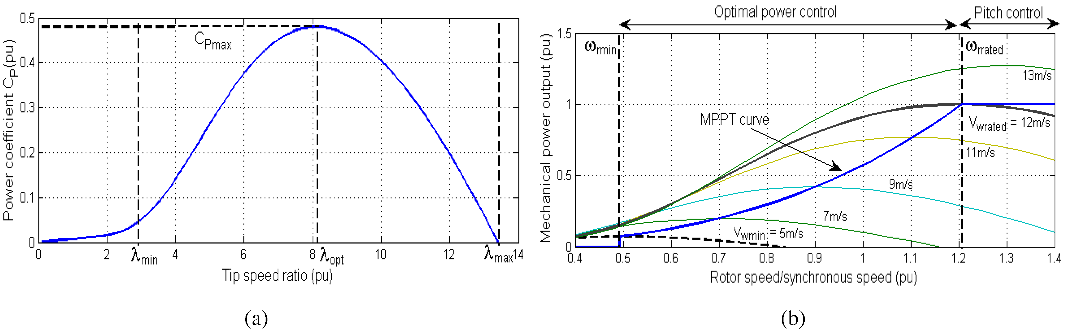
2.1. Wind Turbine
2.2. DFIG
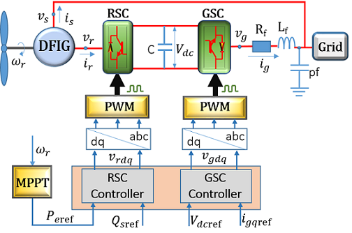
2.3. Converter
3. Controller Design and Maximum Power Strategy
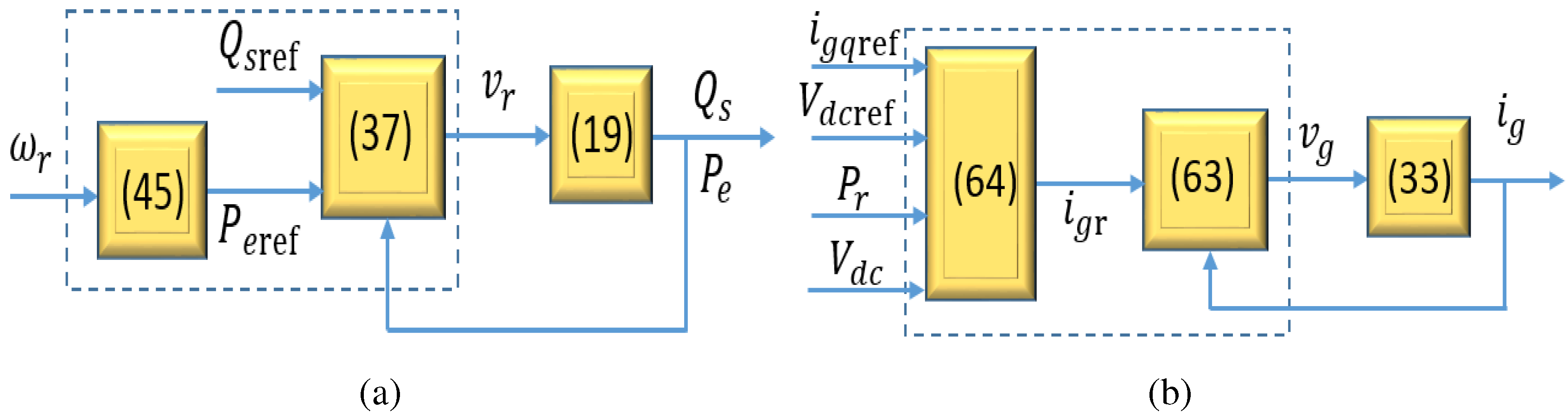
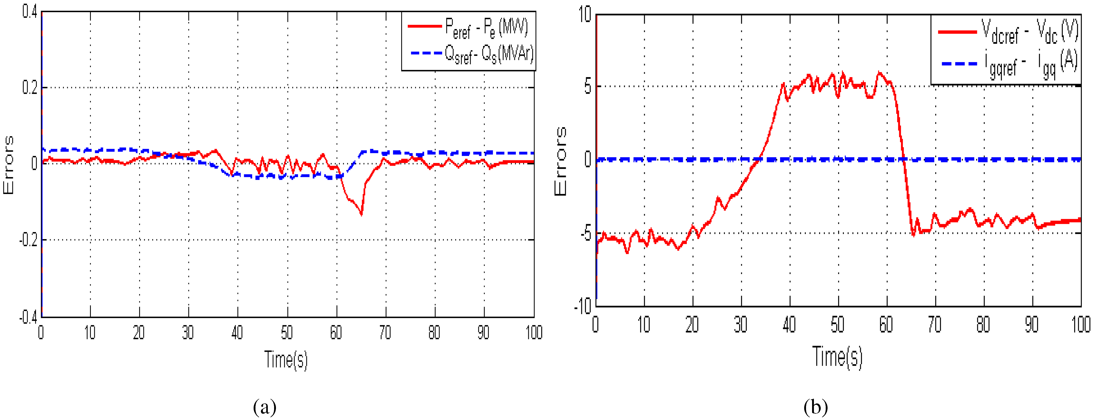
3.1. Rotor-Side Control
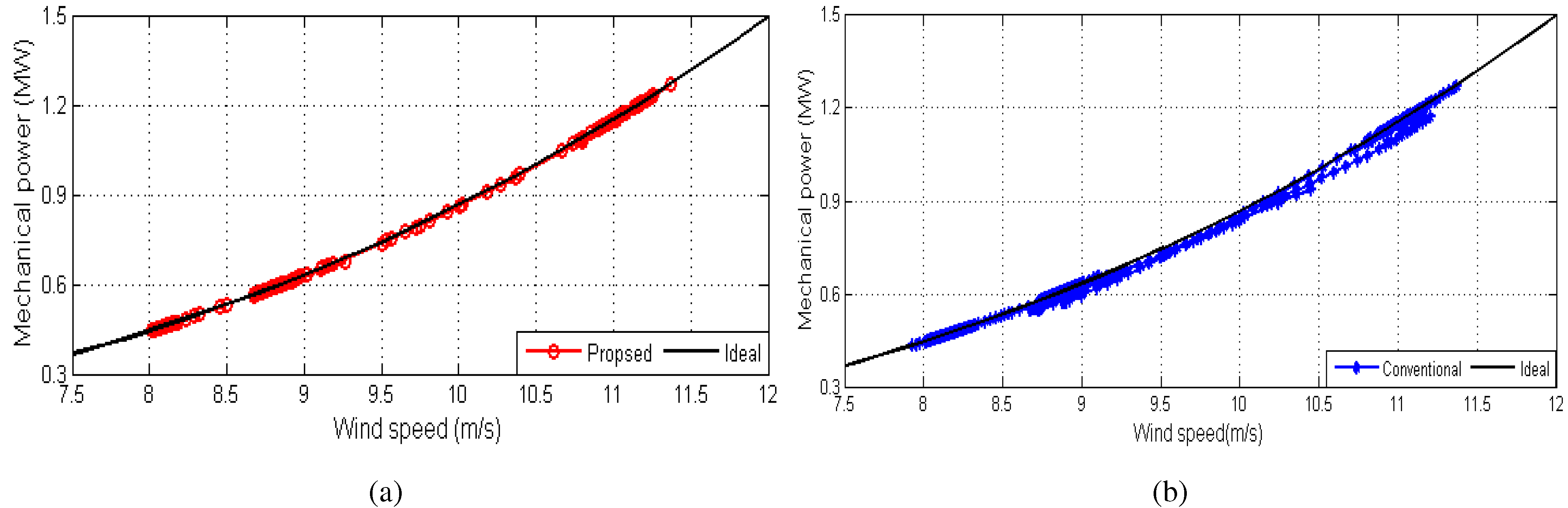
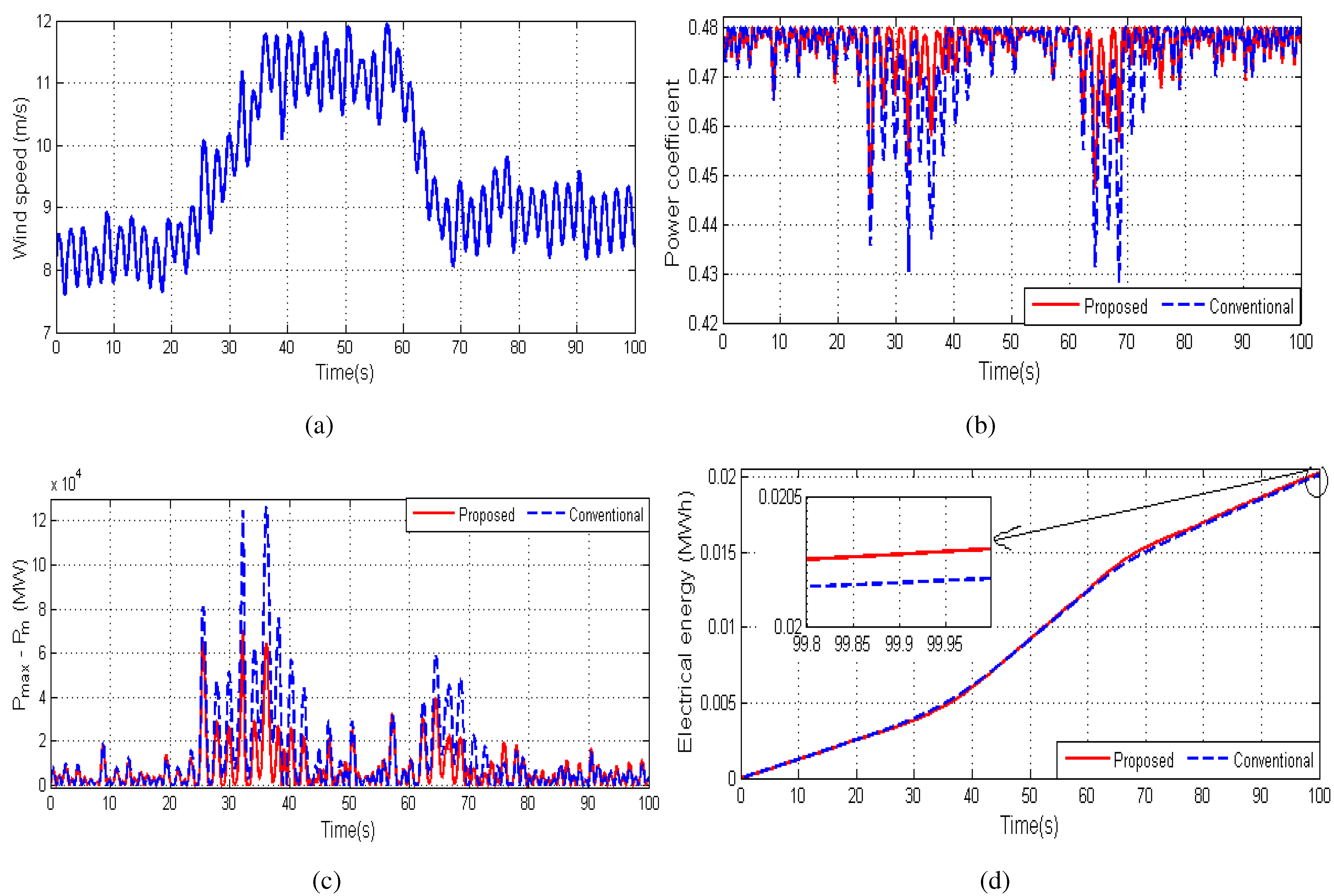
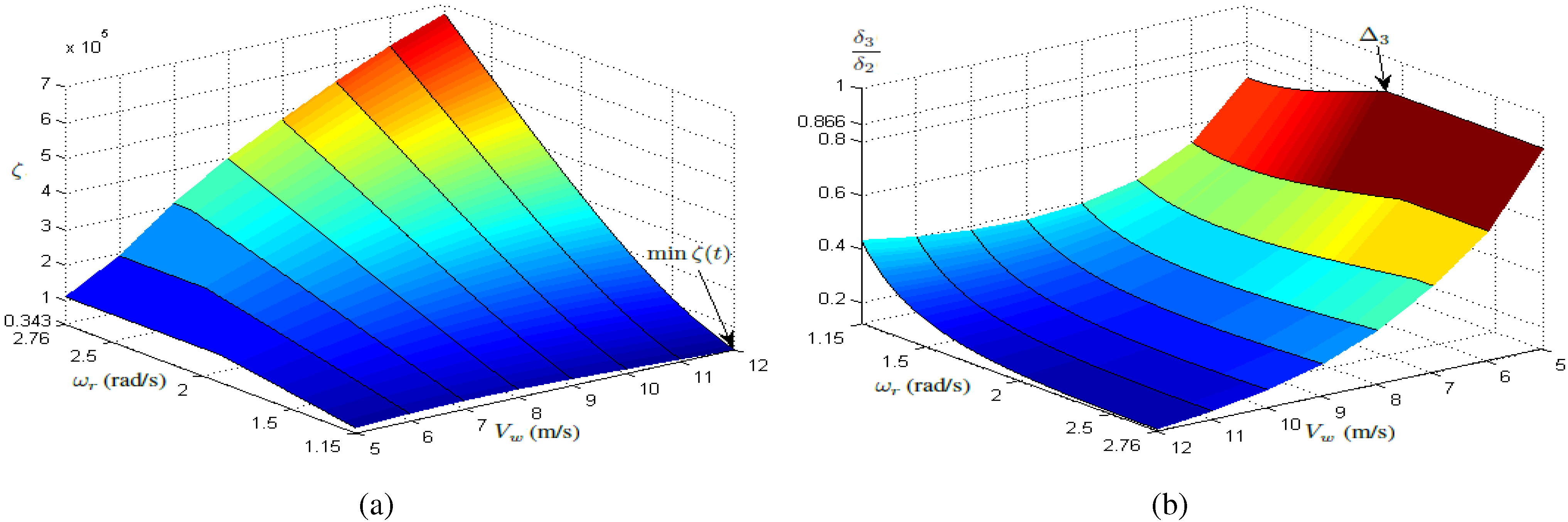
3.2. Maximum Output Power Control
3.3. Grid-Side Control
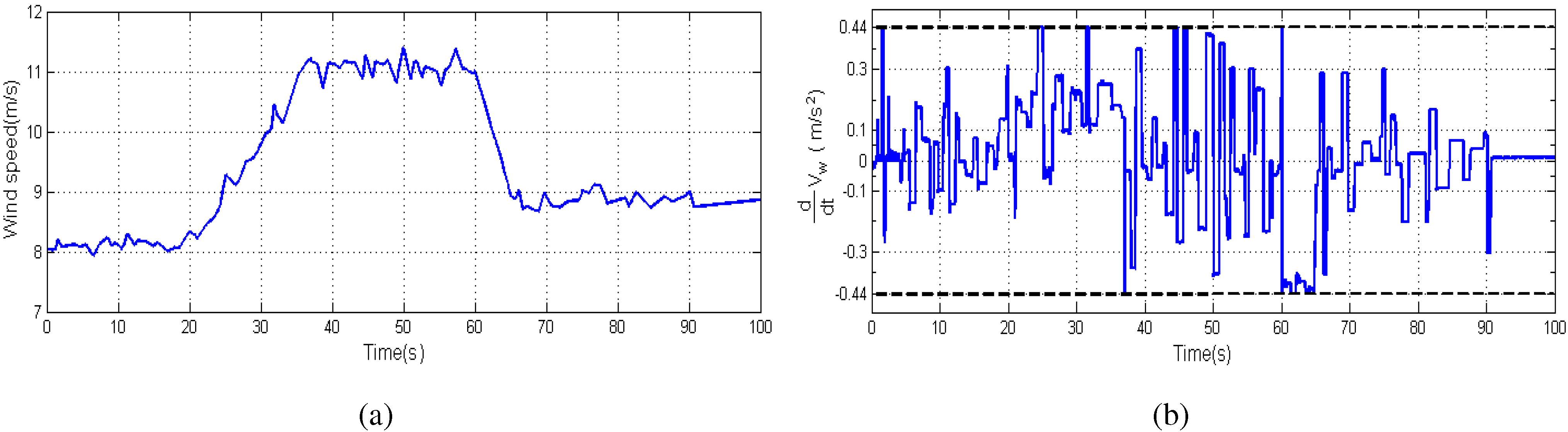
4. Performance Validation

| Name | Symbol | Value | Unit |
|---|---|---|---|
| The length of blade | R | 35.25 | m |
| Rated rotor speed | 22 | rpm | |
| Minimum rotor speed | 11 | rpm | |
| Rated wind speed | 12 | m/s |


5. Conclusions
Author Contributions
Conflicts of Interest
References
- Leon, A.E.; Farias, M.F.; Battaiotto, P.E.; Solsona, J.A.; Valla, M.I. Control strategy of a DVR to improve stability in wind farms using squirrel-cage induction generators. IEEE Trans. Power Syst. 2011, 26, 1609–1617. [Google Scholar] [CrossRef]
- Barakati, S.M.; Kazerani, M.; Aplevich, J.D. Maximum power tracking control for a wind turbine system including a matrix converter. IEEE Trans. Energy Convers. 2009, 24, 705–713. [Google Scholar] [CrossRef]
- Qiu, Y.; Zhang, W.; Cao, M.; Feng, Y.; Infield, D. An electro-thermal analysis of a variable-speed doubly-fed induction generator in a wind turbine. Energies 2015, 8, 3386–3402. [Google Scholar] [CrossRef]
- Abdullah, M.; Yatim, A.H.M.; Tan, C.; Saidur, R. A review of maximum power point tracking algorithms for wind energy systems. Renew. Sustain. Energy Rev. 2012, 16, 3220–3227. [Google Scholar] [CrossRef]
- Ganjefar, S.; Ghassemi, A.; Ahmadi, M. Improving efficiency of two-type maximum power point tracking methods of tip-speed ratio and optimum torque in wind turbine system using a quantum neural network. Energy 2014, 67, 444–453. [Google Scholar] [CrossRef]
- Lei, Y.; Mullane, A.; Lightbody, G.; Yacamini, R. Modeling of the wind turbine with a doubly fed induction generator for grid integration studies. IEEE Trans. Energy Convrers. 2006, 21, 257–264. [Google Scholar] [CrossRef]
- Jeong, H.G.; Seung, R.H.; Lee, K.B. An improved maximum power point tracking method for wind power systems. Energies 2012, 5, 1339–1354. [Google Scholar] [CrossRef]
- Tapia, A.; Tapia, G.; Ostolaza, J.; Saenz, J. Modeling and control of a wind turbine driven doubly fed induction generator. IEEE Trans. Energy Convers. 2003, 18, 194–204. [Google Scholar] [CrossRef]
- Fernandez, L.; Garcia, C.; Jurado, F. Comparative study on the performance of control systems for doubly fed induction generator (DFIG) wind turbines operating with power regulation. Energy 2008, 33, 1438–1452. [Google Scholar] [CrossRef]
- Wagner, H.; Mathur, J. Introduction to Wind Energy Systems: Basics, Technology and Operation; Springer-Verlag: Berlin/Heidelberg, Germany, 2013; pp. 63–64. [Google Scholar]
- Kim, H.W.; Kim, S.S.; Ko, H.S. Modeling and control of PMSG-based variable-speed wind turbine. Electr. Power Syst. Res. 2010, 80, 46–52. [Google Scholar] [CrossRef]
- Yang, L.; Xu, Z.; Stergaard, J.; Dong, Z.Y.; Wong, K.P.; Ma, X. Oscillatory stability and eigenvalue sensitivity analysis of a DFIG wind turbine system. IEEE Trans. Energy Convers. 2011, 26, 328–339. [Google Scholar] [CrossRef]
- Mishra, Y.; Mishra, S.; Li, F.; Dong, Z.Y.; Bansal, R.C. Small signal stability analysis of a DFIG-based wind power system under different modes of operation. IEEE Trans. Energy Convers. 2009, 24, 972–982. [Google Scholar] [CrossRef]
- Hu, J.; Nian, H.; Hu, B.; He, Y.; Zhu, Z.Q. Direct active and reactive power regulation of DFIG using sliding-mode control approach. IEEE Trans. Energy Convers. 2010, 25, 1028–1039. [Google Scholar] [CrossRef]
- Barambones, O.; Cortajarena, J.A.; Alkorta, P.; Durana, J.M.G. A real-time sliding mode control for a wind energy system based on a doubly fed induction generator. Energies 2014, 7, 6412–6433. [Google Scholar] [CrossRef]
- Khemiri, N.; Khedher, A.; Mimouni, M.F. Wind energy conversion system using DFIG controlled by backstepping and sliding mode strategies. Int. J. Renew. Energy Res. 2012, 2, 421–430. [Google Scholar]
- Beltran, B.; Ahmed-Ali, T.; Benbouzid, M. High-order sliding-mode control of variable-speed wind turbines. IEEE Trans. Ind. Electron. 2009, 56, 3314–3321. [Google Scholar] [CrossRef]
- Soliman, M.; Malik, O.P.; Westwick, D.T. Multiple model predictive control for wind turbines with doubly fed induction generators. IEEE Trans. Sustain. Energy 2011, 2, 215–225. [Google Scholar] [CrossRef]
- Wu, B.; Lang, Y.; Zargari, N.; Kouro, S. Power Conversion and Control of Wind Energy System; Wiley: Hoboken, NJ, USA, 2011. [Google Scholar]
- Abad, G.; López, J.; Rodríguez, M.A.; Marroyo, L.; Iwanski, G. Doubly Fed Induction Machine: Modelling and Control for Wind Energy Generation; Hanzo, L., Ed.; John Wiley & Sons: Hoboken, NJ, USA, 2011. [Google Scholar]
- Kim, Y.; Chung, I.; Moon, S. Tuning of the PI controller parameters of a PMSG wind turbine to mmprove control performance under various wind speeds. Energies 2015, 8, 1406–1425. [Google Scholar] [CrossRef]
- Hughes, F. M.; Anaya-Lara, O.; Jenkins, N.; Strbac, G. A power system stabilizer for DFIG-based wind generation. IEEE Trans. Power Syst. 2006, 21, 763–772. [Google Scholar] [CrossRef]
- Singh, M.; Santoso, S. Dynamic models for wind turbines and wind power plants. Available online: http://www.nrel.gov/docs/fy12osti/52780.pdf (accessed on 22 May 2015).
© 2015 by the authors; licensee MDPI, Basel, Switzerland. This article is an open access article distributed under the terms and conditions of the Creative Commons Attribution license (http://creativecommons.org/licenses/by/4.0/).
Share and Cite
Phan, D.-C.; Yamamoto, S. Maximum Energy Output of a DFIG Wind Turbine Using an Improved MPPT-Curve Method. Energies 2015, 8, 11718-11736. https://doi.org/10.3390/en81011718
Phan D-C, Yamamoto S. Maximum Energy Output of a DFIG Wind Turbine Using an Improved MPPT-Curve Method. Energies. 2015; 8(10):11718-11736. https://doi.org/10.3390/en81011718
Chicago/Turabian StylePhan, Dinh-Chung, and Shigeru Yamamoto. 2015. "Maximum Energy Output of a DFIG Wind Turbine Using an Improved MPPT-Curve Method" Energies 8, no. 10: 11718-11736. https://doi.org/10.3390/en81011718
APA StylePhan, D.-C., & Yamamoto, S. (2015). Maximum Energy Output of a DFIG Wind Turbine Using an Improved MPPT-Curve Method. Energies, 8(10), 11718-11736. https://doi.org/10.3390/en81011718