
Power Quality Disturbances Recognition Based on a Multiresolution Generalized S-Transform and a PSO-Improved Decision Tree

Abstract
:1. Introduction
2. Multiresolution Generalized S-Transform
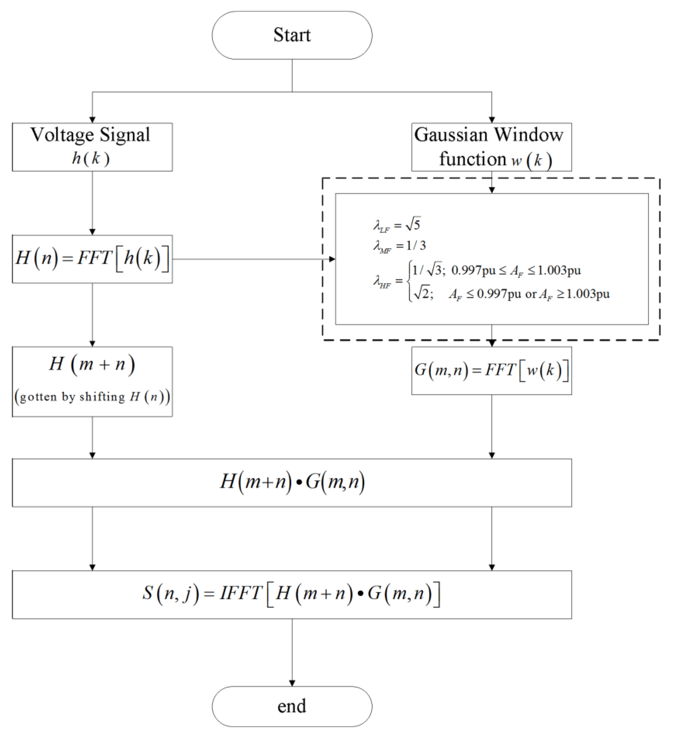
2.1. Generalized S-Transform
2.2. Multiresolution Generalized S-Transform
2.2.1. The Setting of the Width Factor in the Low Frequency Area

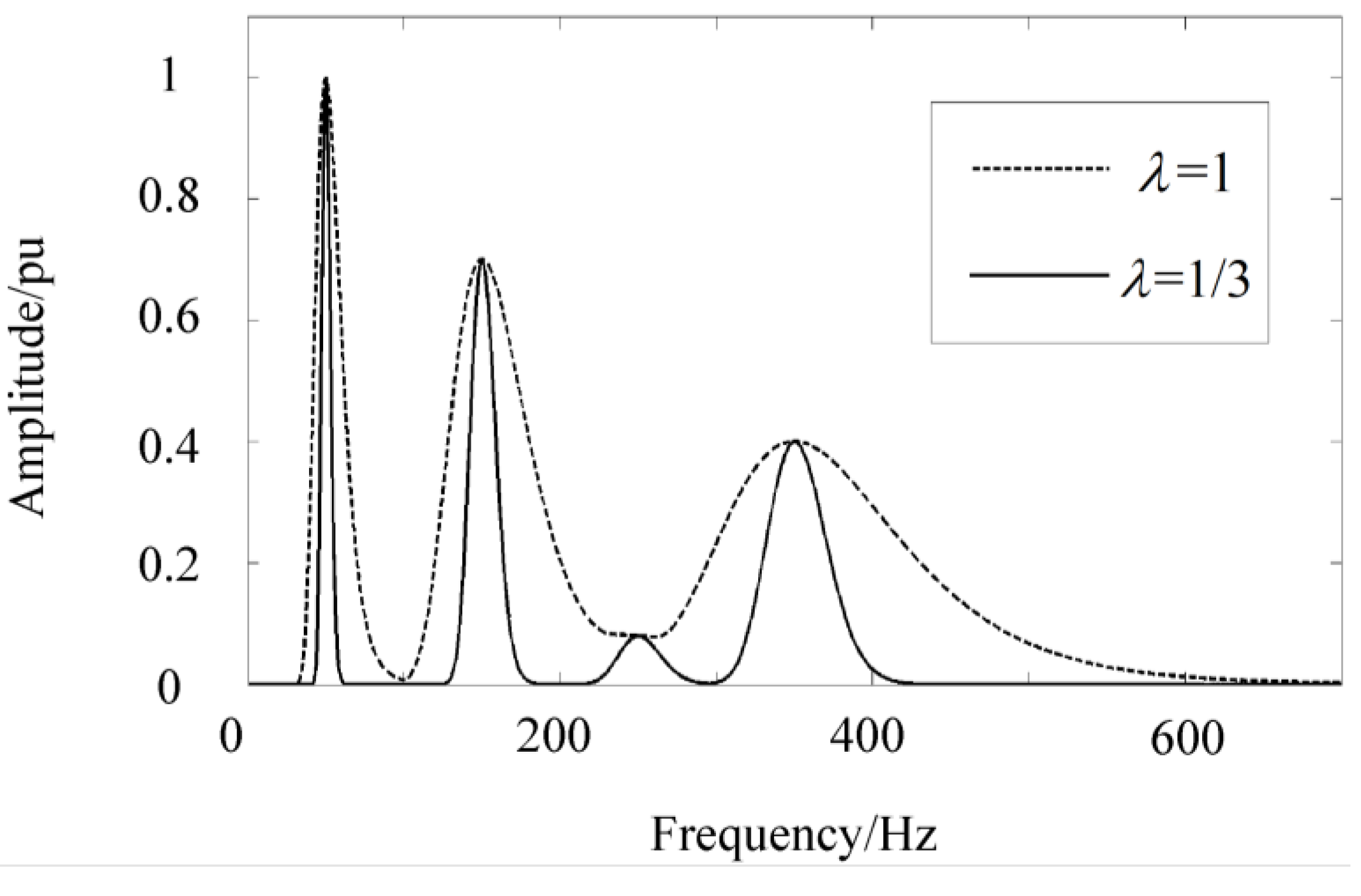
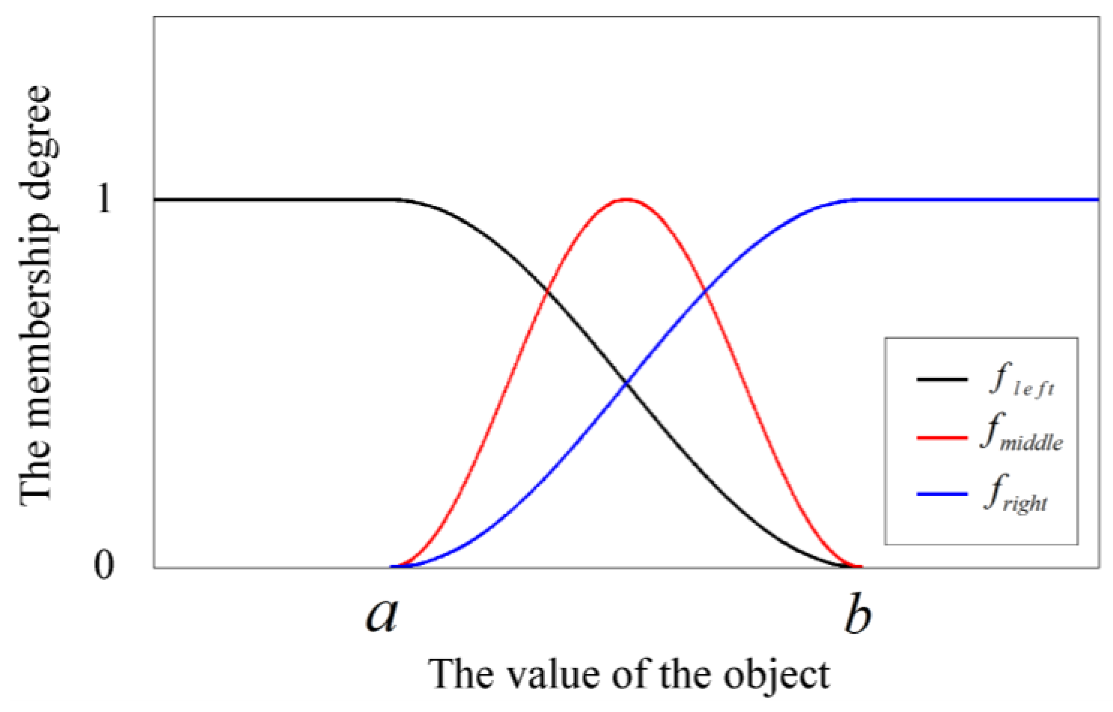
2.2.2. The Setting of the Width Factor in the Middle Frequency Area
2.2.3. The Setting of the Width Factor in the High Frequency Area

3. PQ Disturbance Classifier Based on Decision Tree

| Disturbance Class | Modeling Equations | Equations’ Parameters |
|---|---|---|
| Pure Signal | ||
| Sag | ||
| Swell | ||
| Interruption | ||
| Flicker | ||
| Transient | ||
| Harmonics | ||
| Notch | ||
| Impulse |
| Type of PQ Disturbance | Class Labels |
|---|---|
| Sag | D1 |
| Swell | D2 |
| Interruption | D3 |
| Flicker | D4 |
| Transient | D5 |
| Harmonic | D6 |
| Notch | D7 |
| Impulse | D8 |
| Harmonic with Sag | D9 |
| Harmonic with Swell | D10 |
| Harmonic with Flicker | D11 |
| Harmonic with Transient | D12 |
| Sag with Transient | D13 |
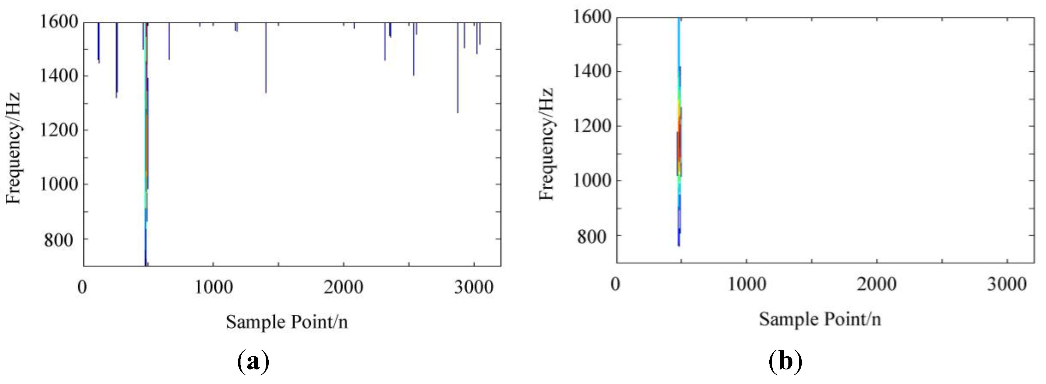
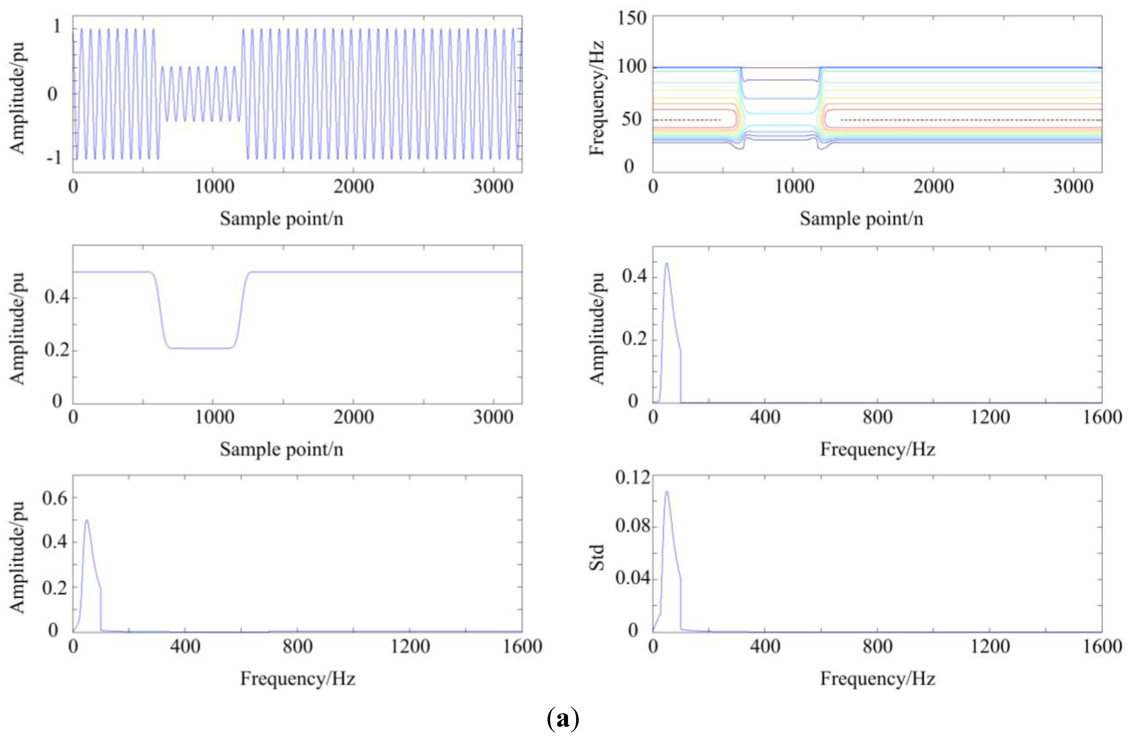
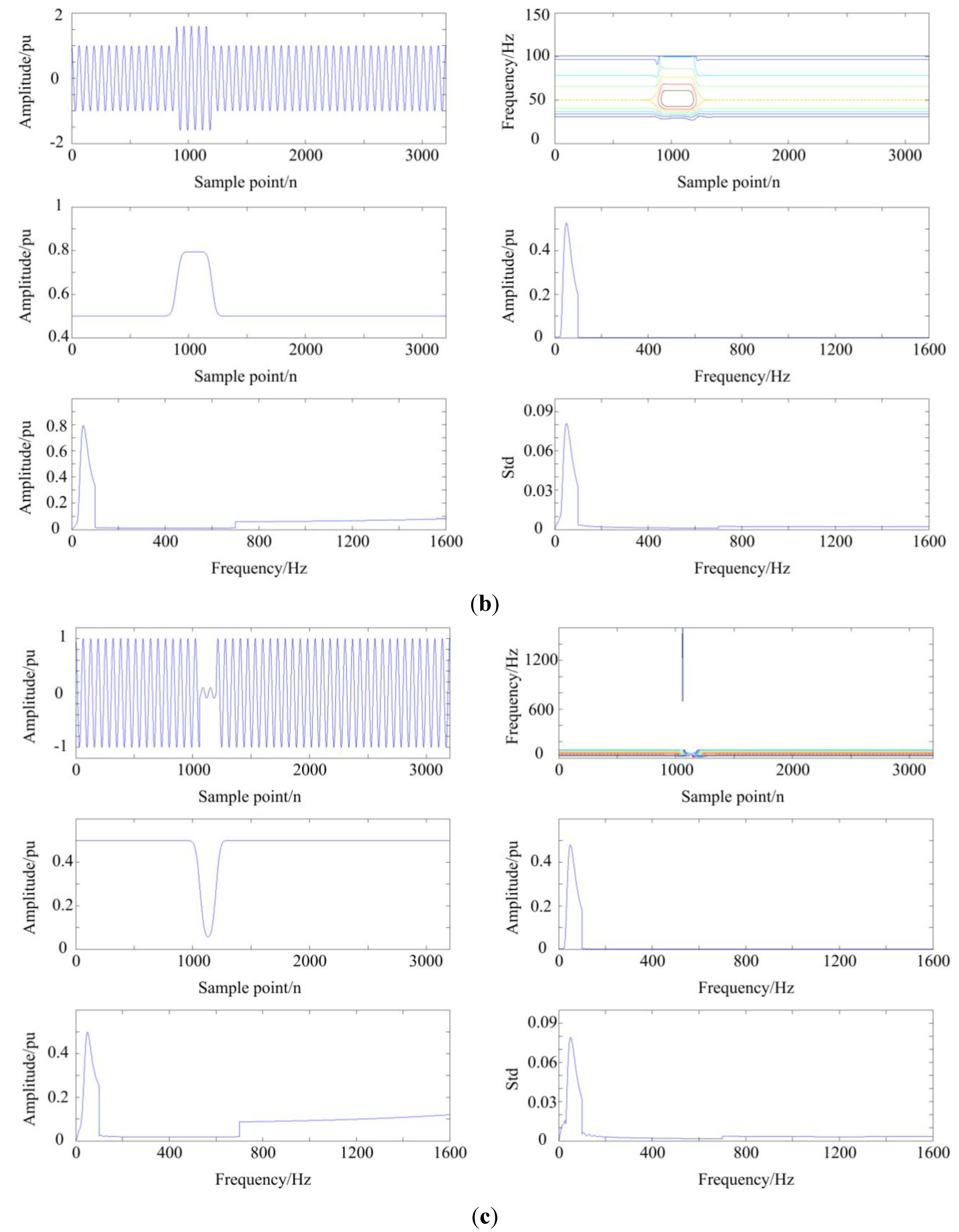
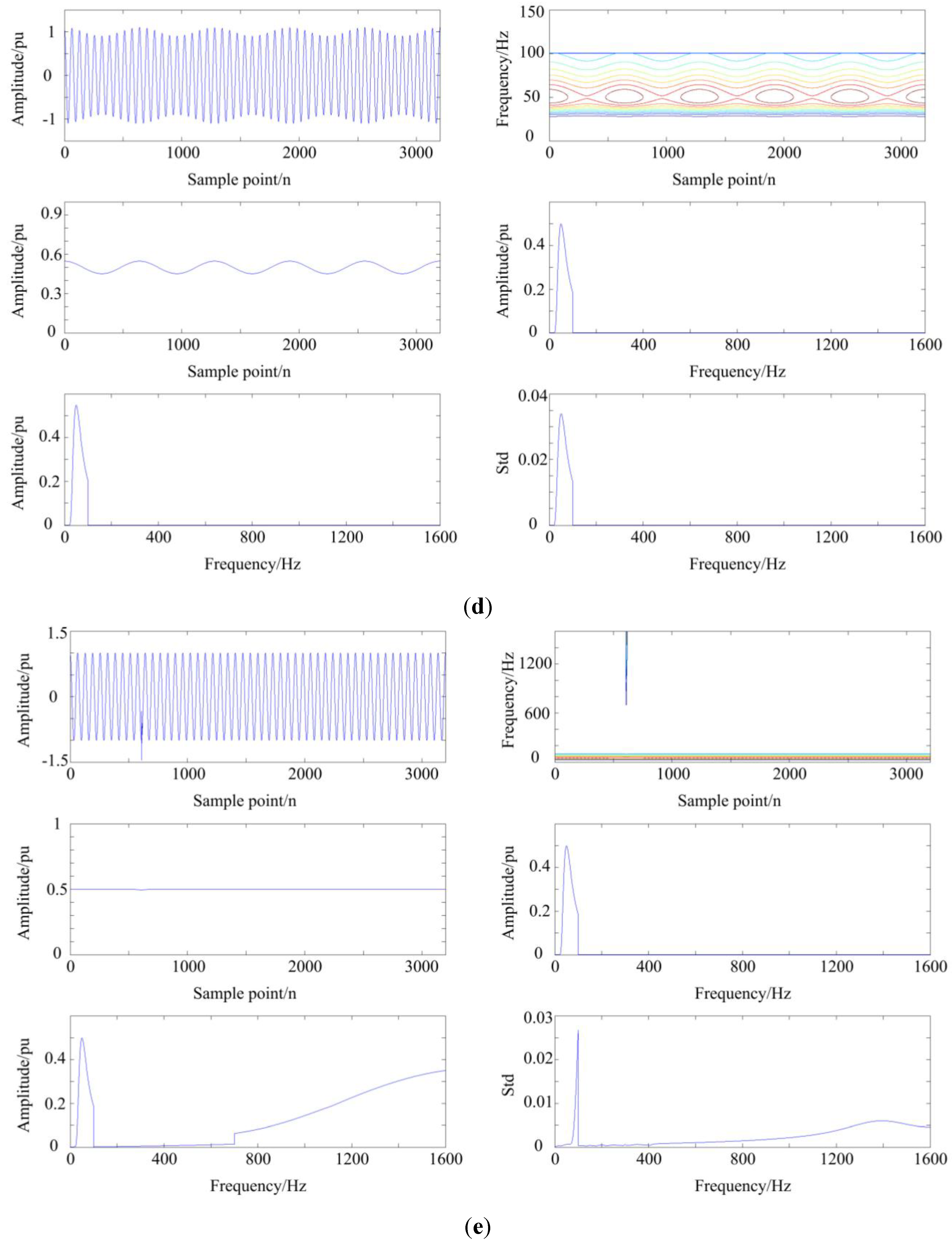
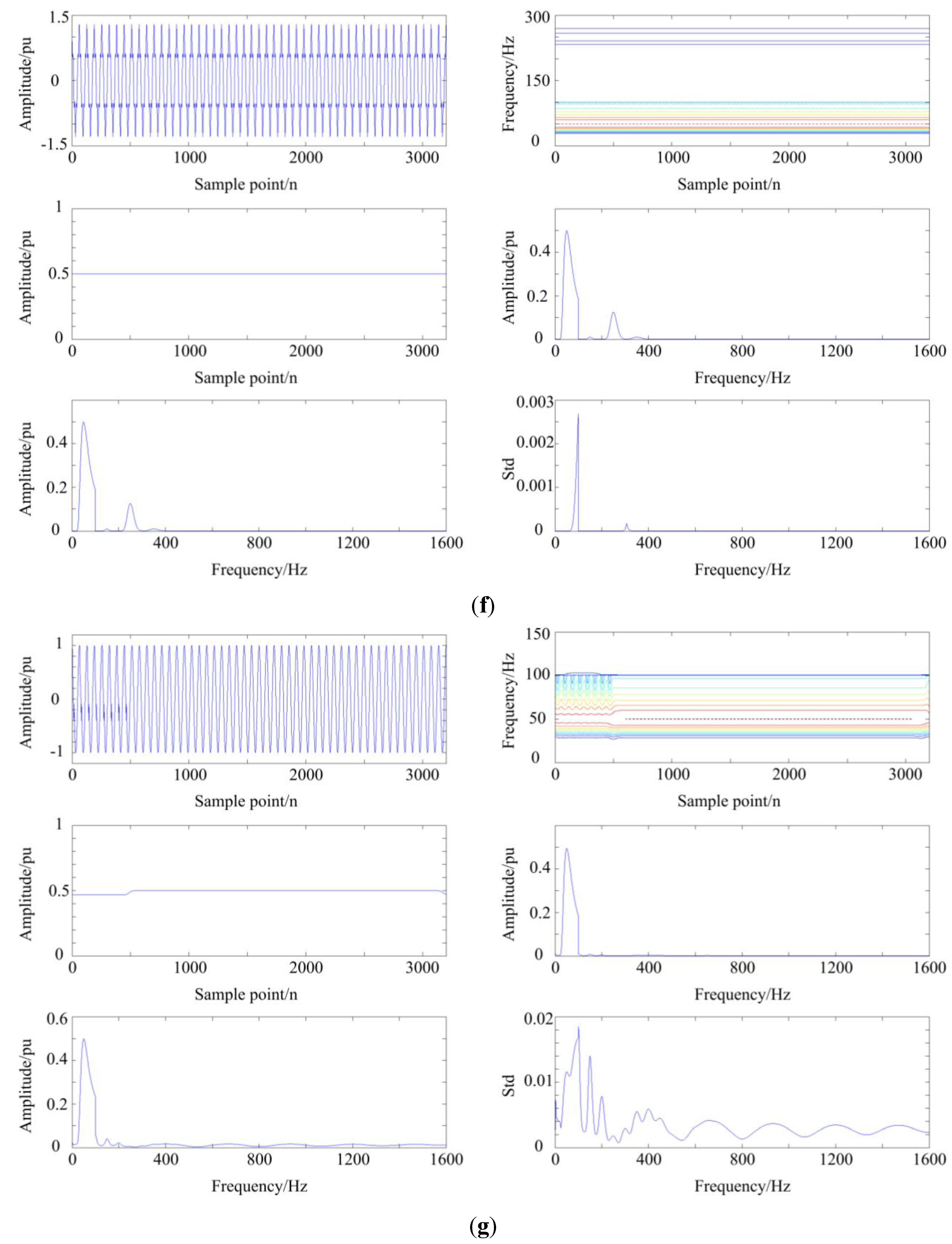
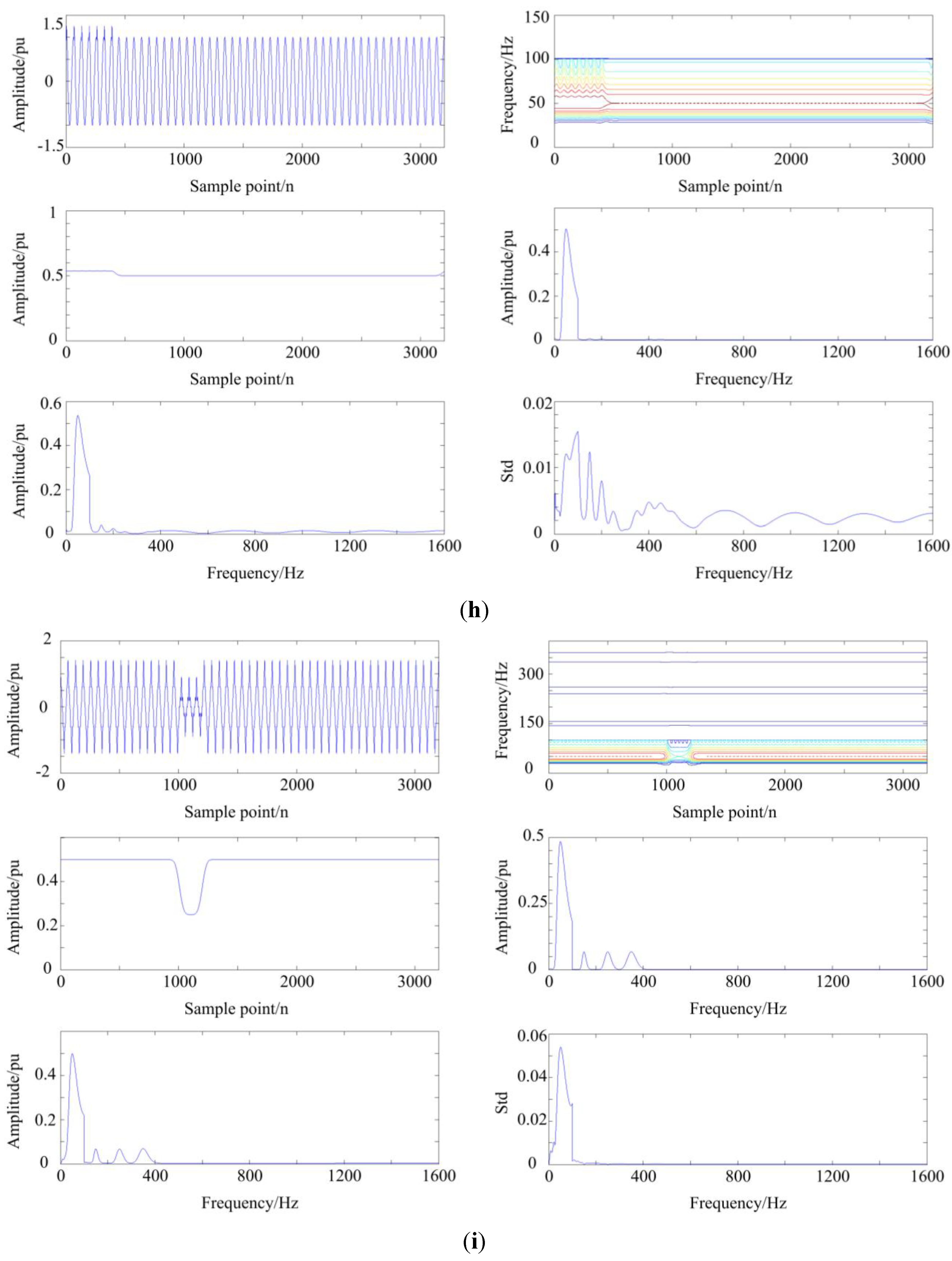
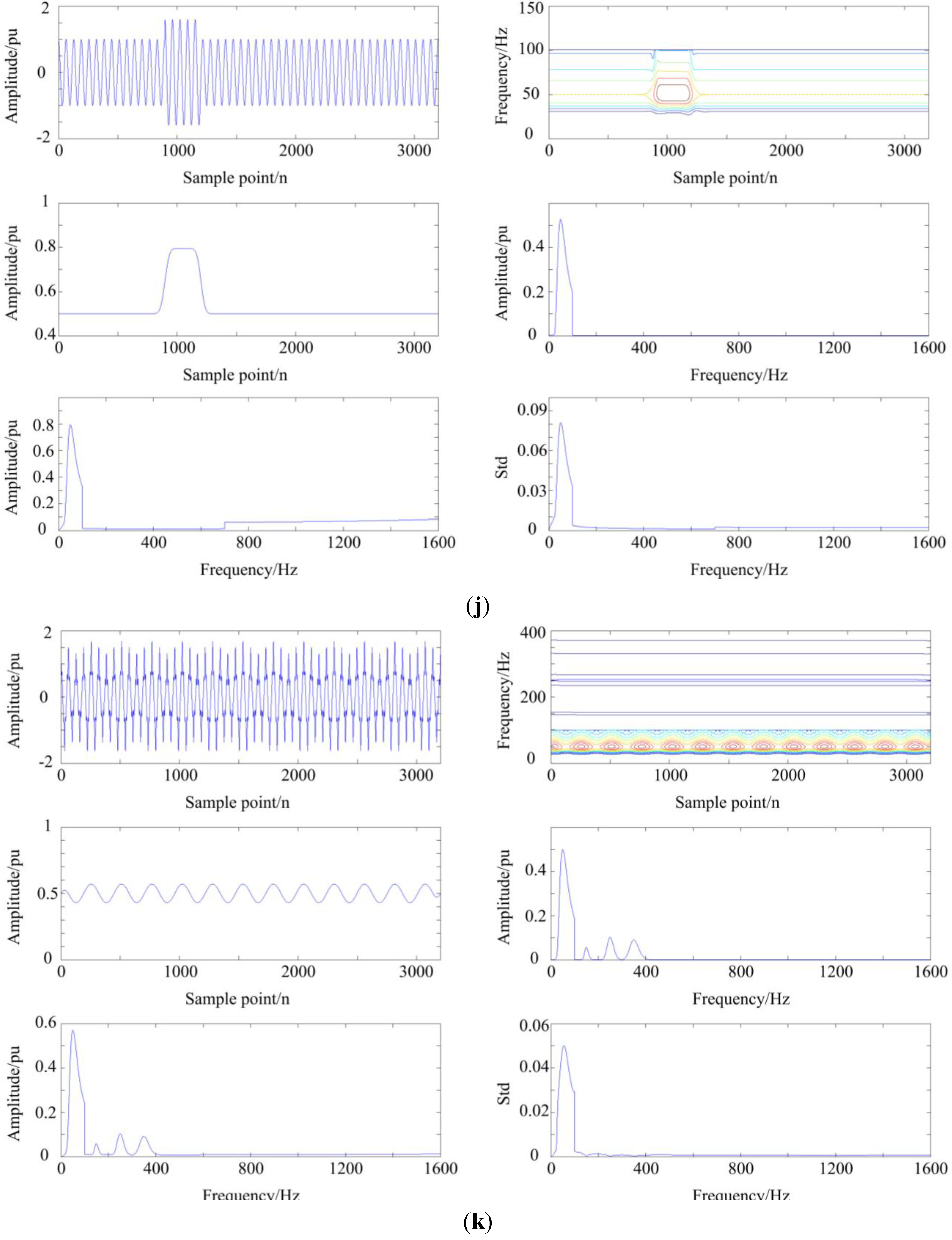
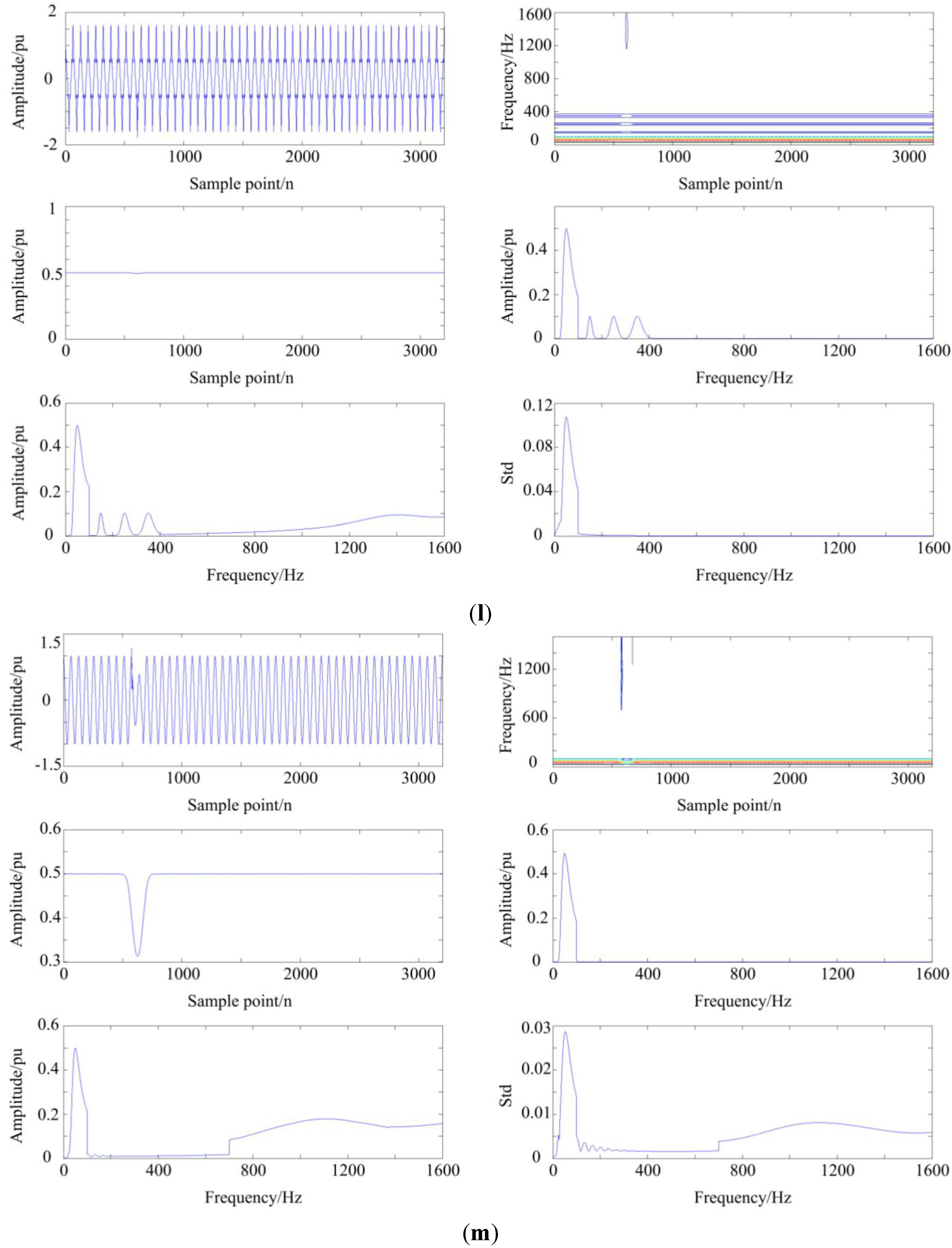
3.1. The Analysis of Disturbance Signal via MGST


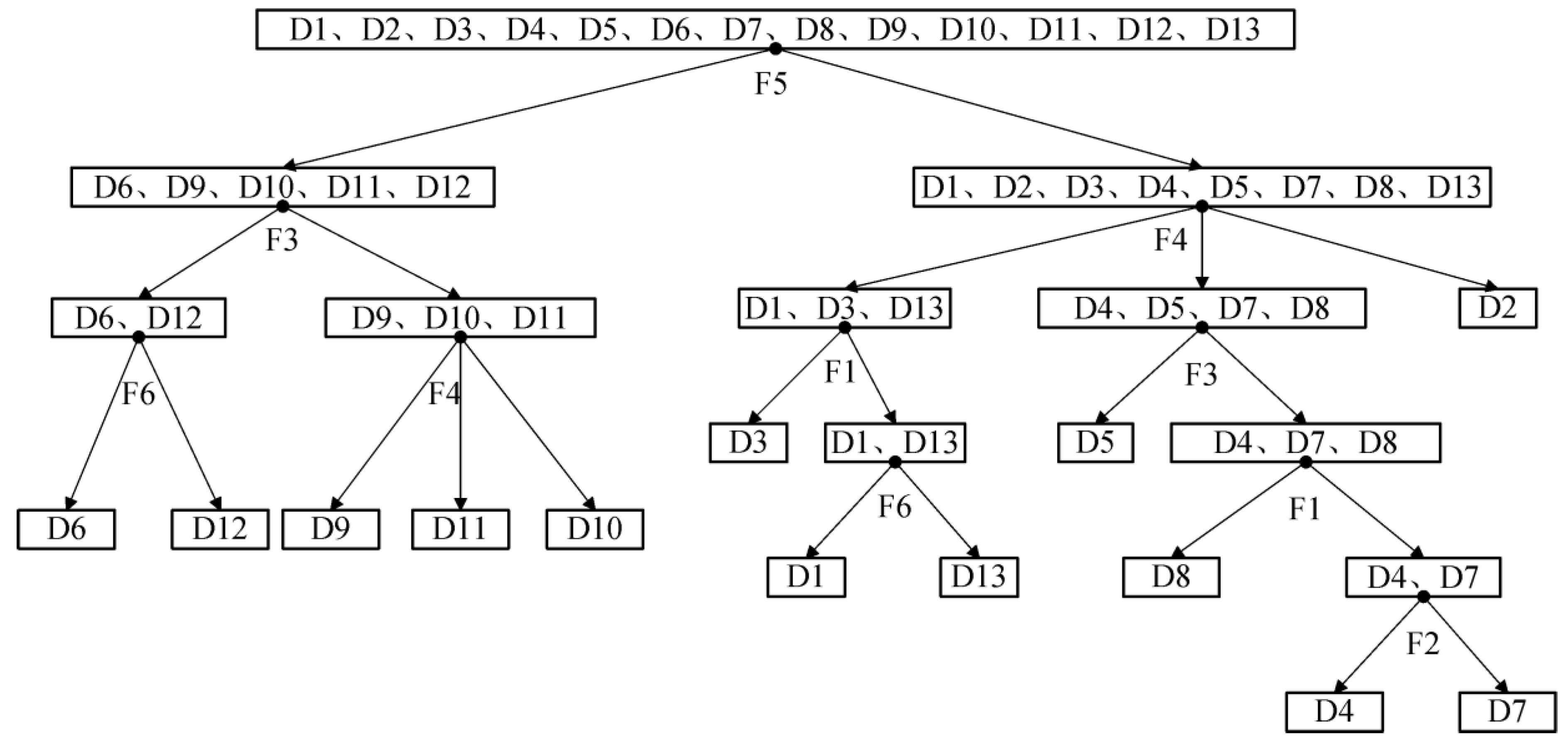
3.2. The Structure of DT
4. Feature Optimization via PSO
4.1. Background
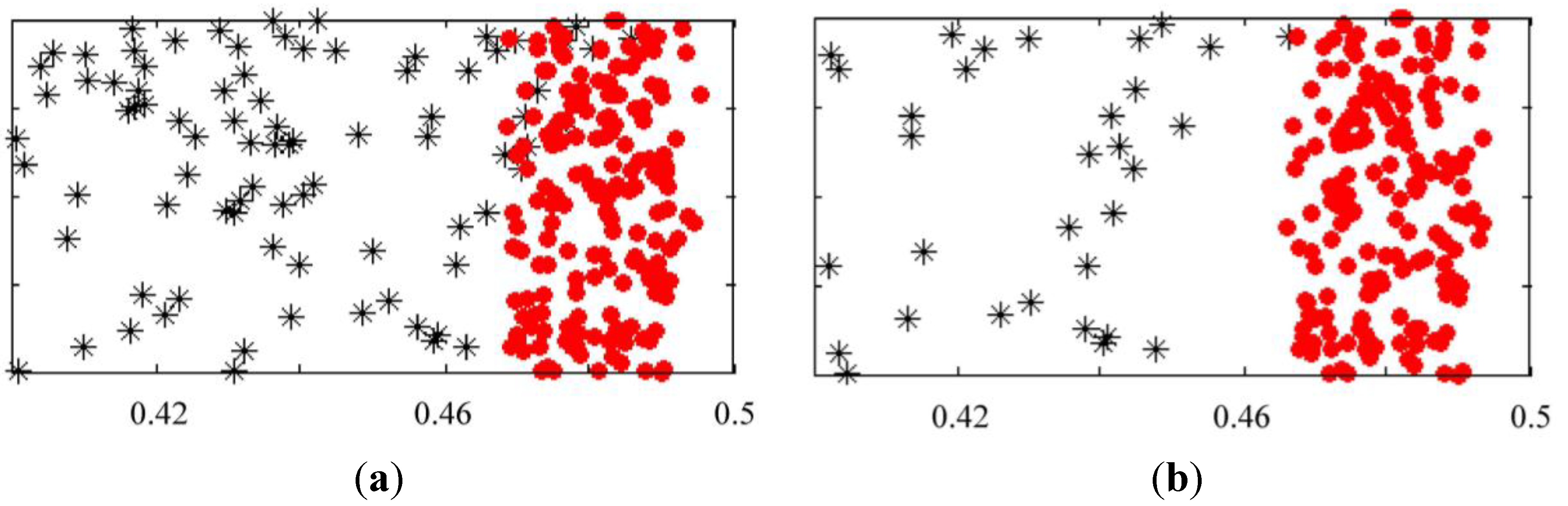
4.2. The Search of Optimized Threshold via Modified PSO
4.2.1. Basic Fundamentals of PSO
4.2.2. The Improvement of PSO
Improvement of the inertia weight
| Inputs & Output | Inputs Fuzzy Sets | Output Fuzzy Set | |
|---|---|---|---|
| Best Fitness Value at Present | Inertia Weight at Present | Percentage Change of the Inertia Weight | |
| RULE1 | LOW | LOW | MEDIUM |
| RULE2 | LOW | MEDIUM | LOW |
| RULE3 | LOW | HIGH | LOW |
| RULE4 | MEDIUM | LOW | HIGH |
| RULE5 | MEDIUM | MEDIUM | MEDIUM |
| RULE6 | MEDIUM | HIGH | LOW |
| RULE7 | HIGH | LOW | HIGH |
| RULE8 | HIGH | MEDIUM | MEDIUM |
| RULE9 | HIGH | HIGH | LOW |
Improvement of the acceleration coefficient
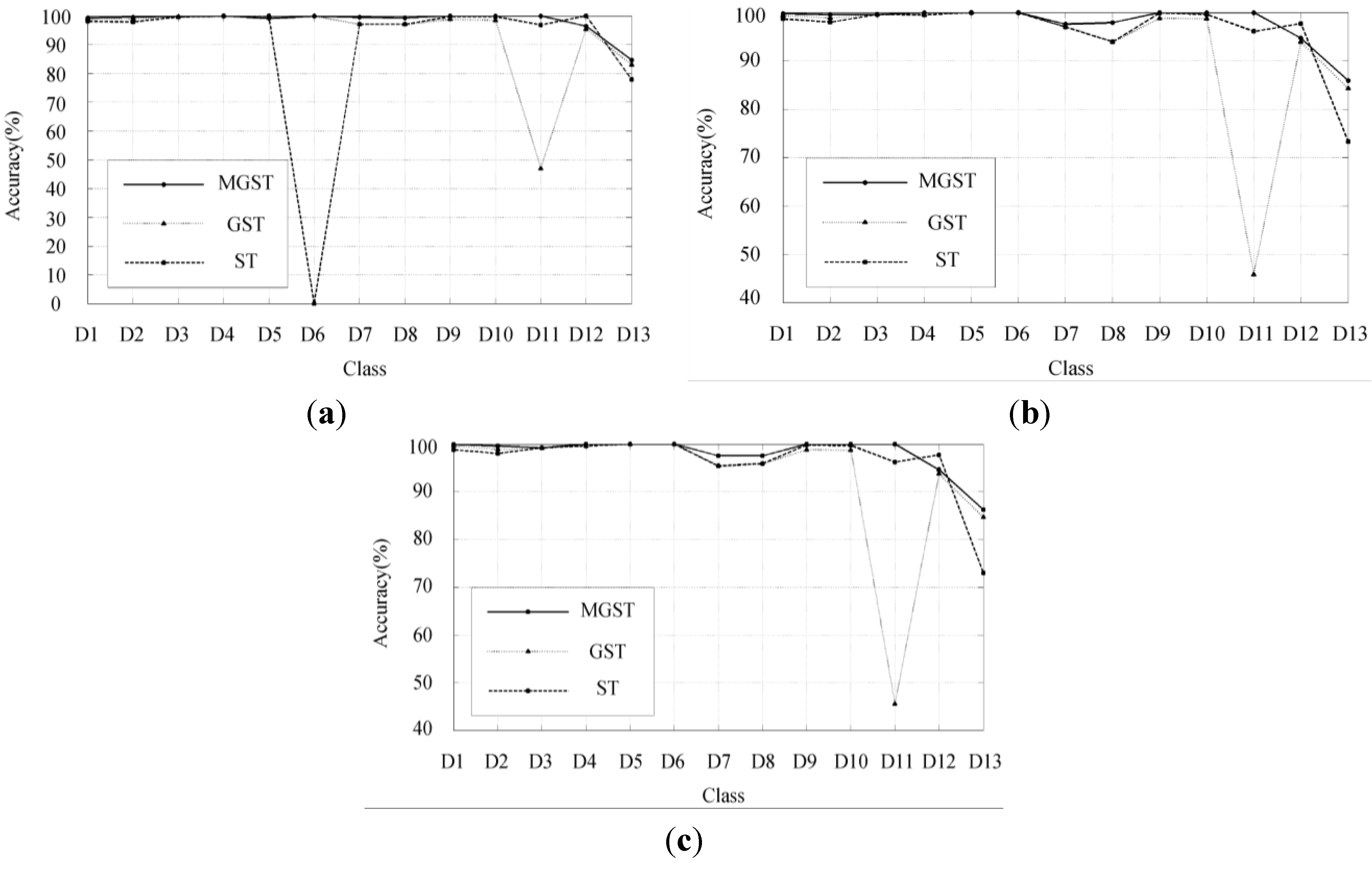
5. Simulation and Experiment
| SNR = 30–50 dB | |||
|---|---|---|---|
| Disturbances | MGST | GST | ST |
| D1 | 99.7 | 99.3 | 98.5 |
| D2 | 99.6 | 98.9 | 98.0 |
| D3 | 99.5 | 99.5 | 99.5 |
| D4 | 100 | 99.7 | 99.7 |
| D5 | 100 | 100 | 100 |
| D6 | 100 | 100 | 93.3 |
| D7 | 99.4 | 97.0 | 97.0 |
| D8 | 99.7 | 96.6 | 96.6 |
| D9 | 100 | 98.8 | 99.8 |
| D10 | 100 | 98.7 | 99.6 |
| D11 | 100 | 45.5 | 96.5 |
| D12 | 94.7 | 93.9 | 98 |
| D13 | 86.4 | 84.9 | 73.4 |
| %Average accuracy | 98.38 | 93.29 | 96.15 |
6. Conclusions
- (1)
- The width factor of the window function in the S-transform is set respectively in different frequency areas, which improves MGST’s ability to recognize complex disturbances.
- (2)
- Features are extracted in different frequency areas so as to avoid the disturbances caused by components of different frequency areas. Moreover, the amount of calculation is reduced.
- (3)
- A cut-off threshold Ts is proposed and optimized by modified PSO, which further improves the anti-noise performance.
- (4)
- Simulation experiments show its effectiveness and practicability.
Acknowledgments
Author Contributions
Conflicts of Interest
References
- Wasiak, I.; Pawelek, R.; Mienski, R. Energy storage application in low-voltage microgrids for energy management and power quality improvement. IET Gener. Transm. Distrib. 2014, 8, 463–472. [Google Scholar] [CrossRef]
- Prodanovic, M.; Green, T.C. High-quality power generation through distributed control of a power park microgrid. IEEE Trans. Ind. Electron. 2006, 53, 1471–1482. [Google Scholar] [CrossRef]
- Baggini, A. Handbook of Power Quality; Wiley Blackwell: New York, NY, USA, 2008. [Google Scholar]
- Saini, M.K.; Kapoor, R. Classification of power quality events—A review. Int. J. Electr. Power Energy Syst. 2012, 43, 11–19. [Google Scholar] [CrossRef]
- Granados-Lieberman, D.; Romero-Troncoso, R.J.; Osornio-Rios, R.A.; Garcia-Perez, A.; Cabal-Yepez, E. Techniques and methodologies for power quality analysis and disturbances classification in power systems: A review. IET Gener. Transm. Distrib. 2011, 5, 519–529. [Google Scholar] [CrossRef]
- Salles, D.; Wilsun, X. Information extraction from PQ disturbances—An emerging direction of power quality research. In Proceedings of the 2012 IEEE 15th International Conference on Harmonics and Quality of Power (ICHQP), Hong Kong, China, 17–20 June 2012; pp. 649–655.
- Farzanehrafat, A.; Watson, N.R. Power Quality State Estimator for Smart Distribution Grids. IEEE Trans. Power Syst. 2013, 28, 2183–2191. [Google Scholar] [CrossRef]
- Gu, Y.H.; Bollen, M.H.J. Time-frequency and time-scale domain analysis of voltage disturbances. IEEE Trans. Power Deliv. 2000, 15, 1279–1284. [Google Scholar] [CrossRef]
- Rodríguez, A.; Aguado, J.A.; Martín, F.; López, J.J.; Muñoz, F.; Ruiz, J.E. Rule-based classification of power quality disturbances using S-transform. Electr. Power Syst. Res. 2012, 86, 113–121. [Google Scholar] [CrossRef]
- Xu, F.; Yang, H.; Ye, M.; Liu, Y.; Hui, J. Classification for power quality short duration disturbances based on generalized S-transform. Proc. Chin. Soc. Electr. Eng. 2012, 4, 77–84. [Google Scholar]
- Biswal, B.; Biswal, M.; Mishra, S.; Jalaja, R. Automatic classification of power quality events using balanced neural tree. IEEE Trans. Ind. Electron. 2014, 61, 521–530. [Google Scholar] [CrossRef]
- Janik, P.; Lobos, T. Automated classification of power-quality disturbances using SVM and RBF networks. IEEE Trans. Power Deliv. 2006, 21, 1663–1669. [Google Scholar] [CrossRef]
- Panigrahi, B.; Pandi, V.R. Optimal feature selection for classification of power quality disturbances using wavelet packet-based fuzzy k-nearest neighbour algorithm. IET Gener. Transm. Distrib. 2009, 3, 296–306. [Google Scholar] [CrossRef]
- Fengzhan, Z.; Rengang, Y. Power-quality disturbance recognition using S-transform. IEEE Trans. Power Deliv. 2007, 22, 944–950. [Google Scholar]
- Kennedy, J.; Eberhart, R. Particle swarm optimization. In Proceedings of the IEEE International Conference on Neural Networks, Perth, Australia, 27 November–1 December 1995; Volume 1944, pp. 1942–1948.
- Eberhart, R.; Kennedy, J. A new optimizer using particle swarm theory. In Proceedings of the Sixth International Symposium on Micro Machine and Human Science (MHS ’95), Nagoya, Japan, 4–6 October 1995; pp. 39–43.
- Stockwell, R.G.; Mansinha, L.; Lowe, R.P. Localization of the complex spectrum: The S transform. IEEE Trans. Signal Process. 1996, 44, 998–1001. [Google Scholar] [CrossRef]
- Pinnegar, C.R.; Mansinha, L. The S-transform with windows of arbitrary and varying shape. Geophysics 2003, 68, 381–385. [Google Scholar] [CrossRef]
- Uyar, M.; Yildirim, S.; Gencoglu, M.T. An expert system based on S-transform and neural network for automatic classification of power quality disturbances. Expert Syst. Appl. 2009, 36, 5962–5975. [Google Scholar] [CrossRef]
- Nguyen, T.; Liao, Y. Power quality disturbance classification utilizing S-transform and binary feature matrix method. Electr. Power Syst. Res. 2009, 79, 569–575. [Google Scholar] [CrossRef]
- Nguyen, T.; Liao, Y. Power quality disturbance classification based on adaptive neuro-fuzzy system. Int. J. Emerg. Electr. Power Syst. 2009, 10. [Google Scholar] [CrossRef]
- Hooshmand, R.; Enshaee, A. Detection and classification of single and combined power quality disturbances using fuzzy systems oriented by particle swarm optimization algorithm. Electr. Power Syst. Res. 2010, 80, 1552–1561. [Google Scholar] [CrossRef]
- Huang, N.; Xu, D.; Liu, X.; Lin, L. Power quality disturbances classification based on S-transform and probabilistic neural network. Neurocomputing 2012, 98, 12–23. [Google Scholar] [CrossRef]
- Chen, D.; Zhao, C. Particle swarm optimization with adaptive population size and its application. Appl. Soft Comput. 2009, 9, 39–48. [Google Scholar] [CrossRef]
- Yuhui, S.; Eberhart, R.C. Fuzzy adaptive particle swarm optimization. In Proceedings of the 2001 Congress on Evolutionary Computation, Seoul, Korea, 27–30 May 2001; Volume 101, pp. 101–106.
- Kennedy, J.; Mendes, R. Neighborhood topologies in fully informed and best-of-neighborhood particle swarms. IEEE Trans. Syst. Man Cybern. C Appl. Rev. 2006, 36, 515–519. [Google Scholar] [CrossRef]
- Ratnaweera, A.; Halgamuge, S.; Watson, H.C. Self-organizing hierarchical particle swarm optimizer with time-varying acceleration coefficients. IEEE Trans. Evol. Comput. 2004, 8, 240–255. [Google Scholar] [CrossRef]
- Wenzhong, G.; Guolong, C.; Xiang, F. A new strategy of acceleration coefficients for particle swarm optimization. In Proceedings of the 10th International Conference on Computer Supported Cooperative Work in Design (CSCWD ’06), Nanjing, China, 3–5 May 2006; pp. 1–5.
© 2015 by the authors; licensee MDPI, Basel, Switzerland. This article is an open access article distributed under the terms and conditions of the Creative Commons Attribution license (http://creativecommons.org/licenses/by/4.0/).
Share and Cite
Huang, N.; Zhang, S.; Cai, G.; Xu, D. Power Quality Disturbances Recognition Based on a Multiresolution Generalized S-Transform and a PSO-Improved Decision Tree. Energies 2015, 8, 549-572. https://doi.org/10.3390/en8010549
Huang N, Zhang S, Cai G, Xu D. Power Quality Disturbances Recognition Based on a Multiresolution Generalized S-Transform and a PSO-Improved Decision Tree. Energies. 2015; 8(1):549-572. https://doi.org/10.3390/en8010549
Chicago/Turabian StyleHuang, Nantian, Shuxin Zhang, Guowei Cai, and Dianguo Xu. 2015. "Power Quality Disturbances Recognition Based on a Multiresolution Generalized S-Transform and a PSO-Improved Decision Tree" Energies 8, no. 1: 549-572. https://doi.org/10.3390/en8010549
APA StyleHuang, N., Zhang, S., Cai, G., & Xu, D. (2015). Power Quality Disturbances Recognition Based on a Multiresolution Generalized S-Transform and a PSO-Improved Decision Tree. Energies, 8(1), 549-572. https://doi.org/10.3390/en8010549