Wind Power Prediction Considering Nonlinear Atmospheric Disturbances

Abstract

This paper considers the effect of nonlinear atmospheric disturbances on wind power prediction. A Lorenz system is introduced as an atmospheric disturbance model. Three new improved wind forecasting models combined with a Lorenz comprehensive disturbance are put forward in this study. Firstly, we define the form of the Lorenz disturbance variable and the wind speed perturbation formula. Then, different artificial neural network models are used to verify the new idea and obtain better wind speed predictions. Finally we separately use the original and improved wind speed series to predict the related wind power. This proves that the corrected wind speed provides higher precision wind power predictions. This research presents a totally new direction in the wind prediction field and has profound theoretical research value and practical guiding significance.

1. Introduction

New energy generally refers to unconventional energy sources, such as wind power, solar power, ocean energy, hydropower, biomass energy, geothermal energy, and so on. In recent years, the development and utilization of new energy has become one of the most important approaches to solve the strain on resources and environmental deterioration. Wind energy, which is clean, renewable, and widely distributed, can be effectively used for large-scale wind power generation. According to statistics from the Global Wind Energy Council (GWEC) [1], global installed wind power capacity had reached 318,117 MW by the end of 2013, which is six times as much as it was 10 years ago. Wind energy is one of the most crucial meteorological factors during wind farm operation [2,3]. The stochastic volatility and intermittent nature of wind energy make wind power possess similar instability. A wide range of wind power integrated into a power system would exert a significant influence on power quality and security. High-precision wind power prediction thus is an imperative for wind energy development.

Lots of mature and stable wind power prediction systems have been developed by international scholars in recent years [4,5,6]. The most representative forecasting systems abroad include the Prediktor system from the Danish National Laboratory, the WPPT system of Technical University of Denmark, the eWind system in the United States, and the AWPPS system in France, etc. The typical prediction systems in China generally include the WINPOP system developed by the China Meteorological Administration, and the WPPS system developed by the Meteorological Service Center in Hubei Province, etc.

According to the different modeling methods used the current wind power prediction models can be divided into physical models, statistical models, artificial intelligence, and hybrid models. Some physical and geographical factors, such as air temperature, atmospheric pressure, atmospheric density, topography and surface roughness, are applied in physical models to obtain wind speed at the axial fan hub. Thus high resolution numerical weather prediction is realized by this means, which is especially suitable for long-term wind power prediction [7,8,9]. Based on large amounts of historical data, statistical models, which generally include the persistence model (PM), time series model (TSM), and Kalman filtering model (KFM), are aimed at establishing a linear relationship between input and output of prediction models [8,10,11]. In recent years, artificial intelligent technology has been widely used in the field of wind power prediction. Artificial intelligence takes many forms such as wavelet neural network (WNN) [12], error back propagation neural network (BP), radial basis function neural network (RBF), support vector machine (SVM) [13], and fuzzy logic (FL) [14]. In order to avoid the limitations of individual forecasting methods, hybrid models are being increasingly proposed in recent years [15,16,17].

WNN, SVM and BP networks are used in this prediction research. The WNN model needs large amounts of historical data to obtain a good prediction result. The BP network, which is especially suitable for small sample wind power prediction, has fast convergence speed and satisfactory performance. SVM has stable predictive ability but low convergence speed. Based on the above three prediction models, the corresponding disturbance models are proposed in this study, which fully consider the nonlinear disturbance effects in the atmosphere system.

This paper is organized as follows: Section 2 overviews the basic dynamics of the Lorenz system. Section 3 describes the modeling data and proposes three new short-term wind speed and power prediction models considering the Lorenz disturbance effect. Section 4 presents the main results of wind speed and power predictions followed with error analysis and introduces the persistence model to evaluate the forecasting performance in this study. Section 5 presents the conclusions of the paper and points out the future work.

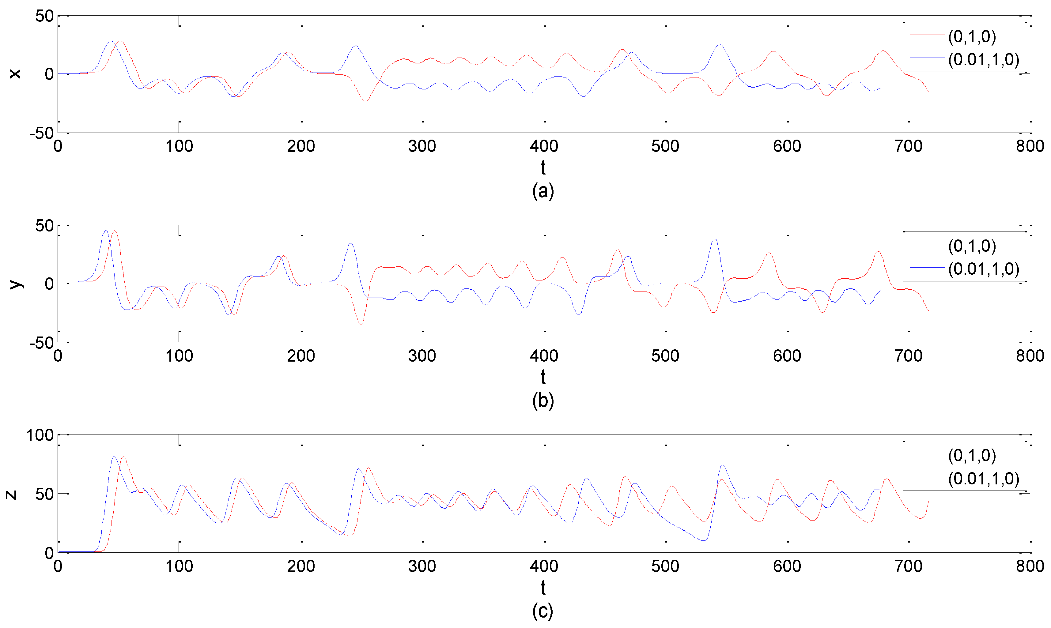
2. Lorenz System and Wind Power Forecasting

It is proven that the wind power generation forecasting errors largely depend on the wind speed [2,8,16,18]. Theoretically, wind speed series containing sensitivity and wind forecasting results could be improved by introducing chaos theory [19,20]. The atmospheric system is a deterministic dynamic system, whose evolution can be described by a set of differential equations. In the meantime, it is also a complex nonlinear system that is filled with uncertainty and chaotic phenomena. According to the butterfly effect viewpoint proposed by E.N. Lorenz [21,22], tiny disturbances may result in a huge variation in the atmospheric system. Then, these random atmospheric disturbances further affect the wind power generation forecasting precision. A Lorenz system could exhibit aperiodic features in the simplest way [21,23]. Thus, we select a Lorenz system to establish our wind disturbance model. The Lorenz equation is given by [23,24,25]:

$$\{\begin{array}{l}\dot{x}=-\text{σ}\left(x-y\right)\\ \dot{y}=-xz+rx-y\\ \dot{z}=xy-bz\end{array}$$

(1)

where x is convection intensity, y is the horizontal temperature difference between the ascending and descending flow, and z is the deviation from vertical temperature difference to equilibrium state. The terms σ, r, and b are all positive parameters. σ is the Prandtl number, which is 10.0 in a liquid and 1.0 in the air [26]. $b=4{(1+a^2)}^{-1}$, and the critical value of r is calculated by:

$$r=\text{σ}(\text{σ}+b+3){(\text{σ}-b-1)}^{-1}$$

(2)

Following Lorenz and Saltzman [23,27], let σ = 10 and a² = 1/2, then b = 8/3, r is variable. Different values of r are used to distinguish the motion state of Lorenz system. Substituting the values of σ and b into Formula (2), r = 470/19 ≈ 24.74. The Lorenz system behaves like a chaotic state when r is larger than 24.74. The chaos describes the random atmospheric perturbations. In this study, the numerical solutions of the Lorenz system are used as disturbance data. In this research we take r = 45.

Now let us show the Lorenz disturbance operation. Let parameters σ, b and r be 10, 8/3, 45, respectively. (0,1,0) and (0.01,1,0) are taken as the initial conditions to solve Equation (1). Figure 1 shows the solutions of the Lorenz equation under the above conditions. We can clearly see that tiny deviations in the initial states could be greatly enlarged as time goes on. The tiny deviation of the initial conditions in Figure 1 amounts to a random disturbance in the atmospheric system. Wind forecasting will become a hard task when considering the sensitivity of wind variation.

This kind of sensitivity is completely non-conducive to accurate wind prediction. We have to take measures to reduce the negative influence of the disturbance. The key point is to quantify the impact as a concrete variable. As mentioned before, Lorenz system is a simplified model for atmospheric convection motion. We can extract a certain kind of disturbance from the solutions of Lorenz equation. The detailed extraction will be presented in the following section.

Figure 1. The subplots (a), (b) and (c) separately depict the solutions x, y and z in Lorenz system. Parameters σ = 10, b = 8/3, r = 45. The red and blue curves denote the solutions developing with initial conditions (0,1,0) and (0.01,1,0), respectively.

Figure 1. The subplots (a), (b) and (c) separately depict the solutions x, y and z in Lorenz system. Parameters σ = 10, b = 8/3, r = 45. The red and blue curves denote the solutions developing with initial conditions (0,1,0) and (0.01,1,0), respectively.

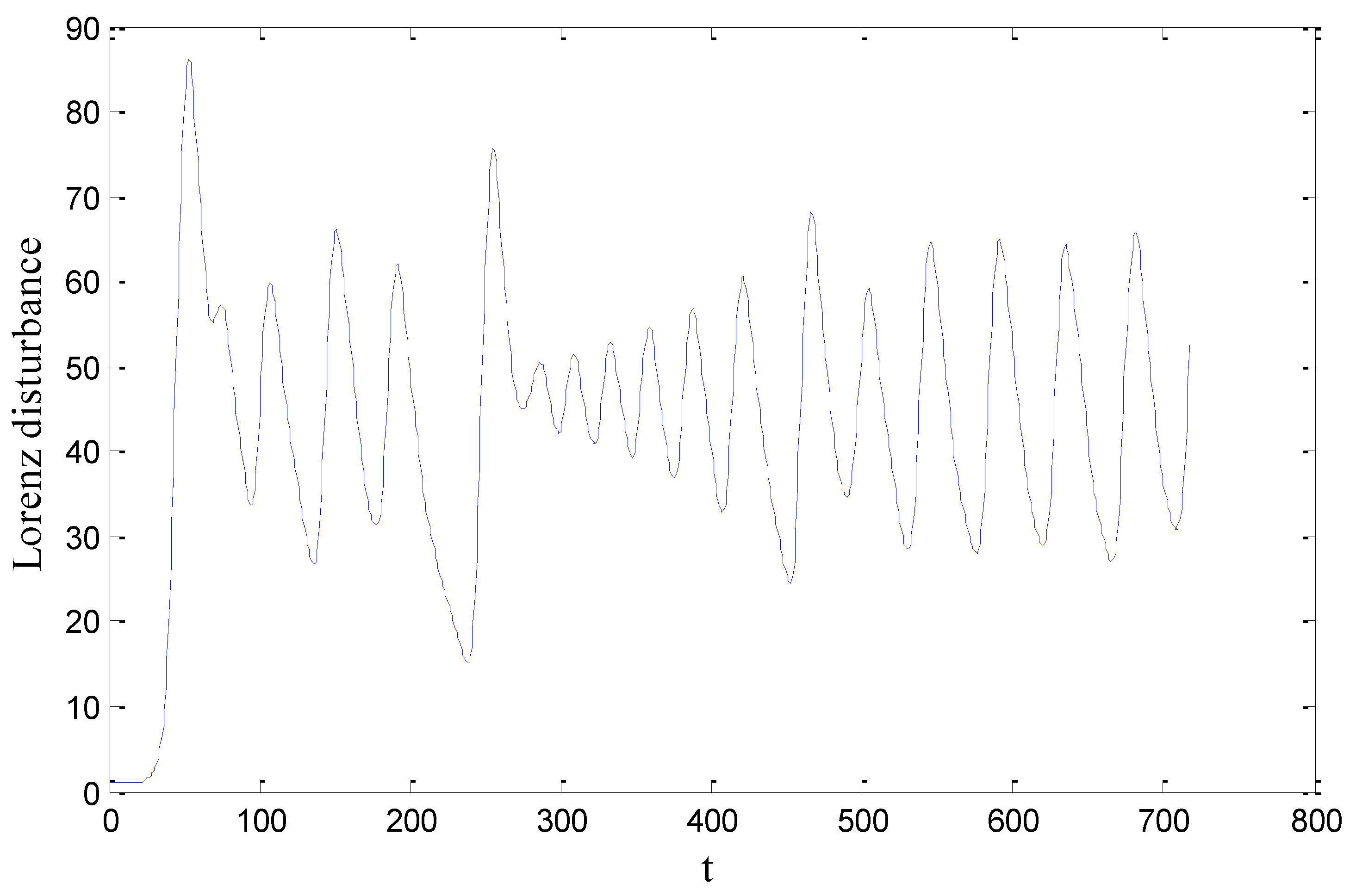
3. Wind Power Prediction Based on a Nonlinear Lorenz Disturbance

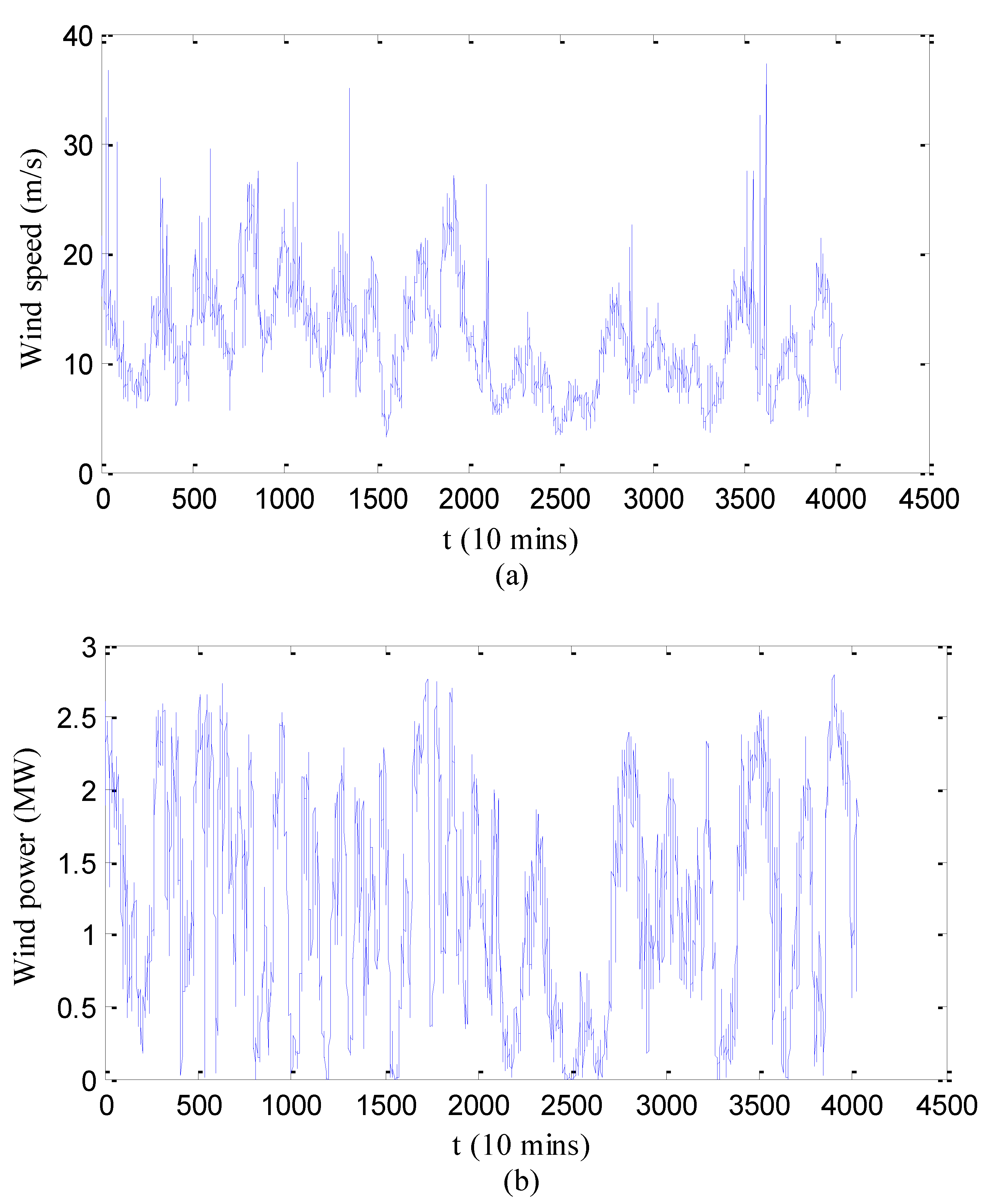
3.1. Data Description

The primary modeling data includes wind speed, wind direction, and power generation. These comprehensive statistics are available from the Sotavento experimental wind farm in Galicia (Spain). All the wind data used in this research were recorded every 10 min in February 2014. The number of samples is 4032. There are four null values at the moment of sharp fluctuations in the wind speed series. The null values are looked at as the random disturbance, which can be deleted without affecting the characteristics of the original wind distribution. Then the sample number is 4028. The displayed wind sample data include wind speed and wind power generation. Figure 2a,b separately depict the distributions of wind speed and wind power production. As we can see from Figure 2a, wind speed fluctuates wildly in February, with a range of 33.96 m/s. Influenced by the wind speed, the wind power presents instability. We can respectively identify the training dataset and test dataset as A and B for convenience. The dataset A contains 3940 points and B contains 88 points. All the experiments have the same forecasting period and different training subsets.

Figure 2. (a) Wind speed distribution in February 2014 of the Sotavento wind farm; (b) Wind power distribution in February 2014 of the Sotavento wind farm.

Figure 2. (a) Wind speed distribution in February 2014 of the Sotavento wind farm; (b) Wind power distribution in February 2014 of the Sotavento wind farm.

3.2. Modeling Process for Wind Power Prediction

As already seen from Figure 1, any tiny deviation that occurred in a nonlinear atmospheric system shall make a huge difference in the subsequent atmospheric evolution. The inevitable atmospheric disturbance is a typical nonlinear process, which will exert significant influence on wind power prediction. An indirect wind power prediction method that forecasts wind speed at the first step is applied in this paper. Based on the predicted wind speed and the corresponding sample data, a new disturbance model is proposed to further optimize the initial wind forecasting result. Then the optimized wind speeds are used to directly predict wind power generation through various prediction models. Wind power prediction can be divided into the following four steps to realize:

The first step is to numerically solve Lorenz equation so as to obtain a nonlinear atmospheric disturbance sequence. Following the analysis aforementioned, the initial condition takes the value of (0,1,0) and the parameters are set as σ = 10, b = 8/3, r = 45.

The second step is to define a kind of Lorenz comprehensive disturbance, which fully considers the influence of all the Lorenz variables. As we know, motion analysis in phase space has the advantage of intuitive geometry. So the phase space R³ expanded by the state variables of the Lorenz system is adopted in this study. An arbitrary point P(x,y,z) in phase space represents a corresponding motion state in Lorenz system. In R³ space, Euclidean distance is the most commonly used measurement of the distance between two points P_i(x_i,y_i,z_i) and P_j(x_j,y_j,z_j). Given by:

$$d\left(p_i,p_j\right)=\Vert p_i-p_j\Vert =\sqrt{{\left(x_i-x_j\right)}^2\text{+}{\left(y_i-y_j\right)}^2\text{+}{\left(z_i-z_j\right)}^2},i,j=1,2,\cdots$$

(3)

In this paper, we set the length of vectors in phase space as the comprehensive disturbance L, which represents the deviation from equilibrium state P₀(0,0,0) to an arbitrary motion state in the perturbed system. Based on the perturbation series produced in step one and Formula (3), L can be calculated. Figure 3 depicts the distribution of L:

$$L=\Vert p_i\Vert =\sqrt{{x_i}^2{{\text{+y}}_i}^2{{\text{+z}}_i}^2}$$

(4)

Figure 3. The distribution of the Lorenz comprehensive disturbance L.

Figure 3. The distribution of the Lorenz comprehensive disturbance L.

The third step is to establish wind speed perturbation models. In order to verify the effectiveness and universality of the disturbance method, based on WNN, BP and SVM models, the corresponding perturbation models denoted as LSWNN, LSBP and LSSVM are proposed. Here we take the LSBP network as an example to explain the modeling process, with which the other two networks are completely similar.

At first, wind speed, sine and cosine of wind direction, air temperature and pressure are chosen as the input of the LSBP network. The output is the wind speed at the next moment. Wind speed data in A are used to train the BP network. Scroll to predict the subsequent 86-points through the trained network above and finally obtain the initial wind speed predicted sequence V_f.

Then we establish the disturbance model based on the BP network, namely the LSBP network. Lorenz disturbance L is used to disturb and modify the predicted sequence V_f. The perturbation formula is given by:

$$V=V_f\pm k\cdot L_f$$

(5)

where, V is the corrected wind speed, k is the disturbance coefficient and L_f is a certain part of the Lorenz disturbance L. Then k·L_f is the quantity that is used to refine the initial wind speed prediction result. It is closely connected with the distribution feature of V_f ± denotes enhancing or reducing the Lorenz disturbance. We will discuss how to select the sign in next section.

According to the report by Lorenz named The Butterfly Effect [21], the real atmospheric motion state is composed of the observed values and a certain disturbance quantity. The perturbation Formula (5) was given based on the above atmospheric disturbance theory. In this paper, the sample data and the predicted values are all generalized observations. Then we need to find the disturbance related to the observations. According to Formula (5), the disturbance consists of two parts: the disturbance coefficient and intensity. The selection of the disturbance coefficient is limited to a certain symmetric interval, such as (−6, 6). Then we divide the interval into some equal parts. The values at the nodes are taken as the coefficients. Then we select the corresponding disturbance intensity from the Lorenz disturbance sequence L. Large amounts of the original wind data need to be repeatedly trained using the LSBP network to achieve the minimum root mean square error (RMSE) between V_f and the wind speed sample data. Then we can obtain an optimal group of disturbance coefficients and intensity through a two-dimensional search. The disturbance is assumed to be the right one that the actual wind speed series contain. It can also be applied in Formula (5) to predict the wind speed series, which have the same or similar distribution with the data used in this paper.

Finally, we have to emphasize once again that this is an example to establish the other two perturbation models LSWNN and LSSVM. The detailed applications of the Lorenz disturbance in the above three perturbation models are shown in Table 1. Thus, the integration of wind speed forecasting and correction is realized through this process. In spite of the use of the same forecasting period, the three models have different initial predictions. Thus we have to use different amount of disturbance and perturbation directions (enhanced or reduced) to deal with those V_f s, which are closely related with the properties of prediction models. Besides, the PM is introduced as a benchmark to measure the forecasting levels.

The fourth step is to forecast the corresponding wind power series based on the improved wind speed prediction result Vs. Then V and V_f obtained by the LSBP model are separately used as the input of the BP wind power prediction model. The same procedure is applied to the WNN and SVM wind power prediction models. As a result, three groups of wind power predictions are obtained. PM is also used to evaluate the precision of wind power predictions.

Table 1. The distribution of the Lorenz disturbance added in the perturbation models LSWNN, LSBP and LSSVM.

Perturbation models	Lorenz disturbance	Data or charts
LSWNN	Disturbance coefficient	0.0253
	Disturbance intensity
LSBP	Disturbance coefficient	−0.0384
	Disturbance intensity
LSSVM	Disturbance coefficient	−0.0131
	Disturbance intensity

Table 1. The distribution of the Lorenz disturbance added in the perturbation models LSWNN, LSBP and LSSVM.

Perturbation models	Lorenz disturbance	Data or charts
LSWNN	Disturbance coefficient	0.0253
	Disturbance intensity
LSBP	Disturbance coefficient	−0.0384
	Disturbance intensity
LSSVM	Disturbance coefficient	−0.0131
	Disturbance intensity

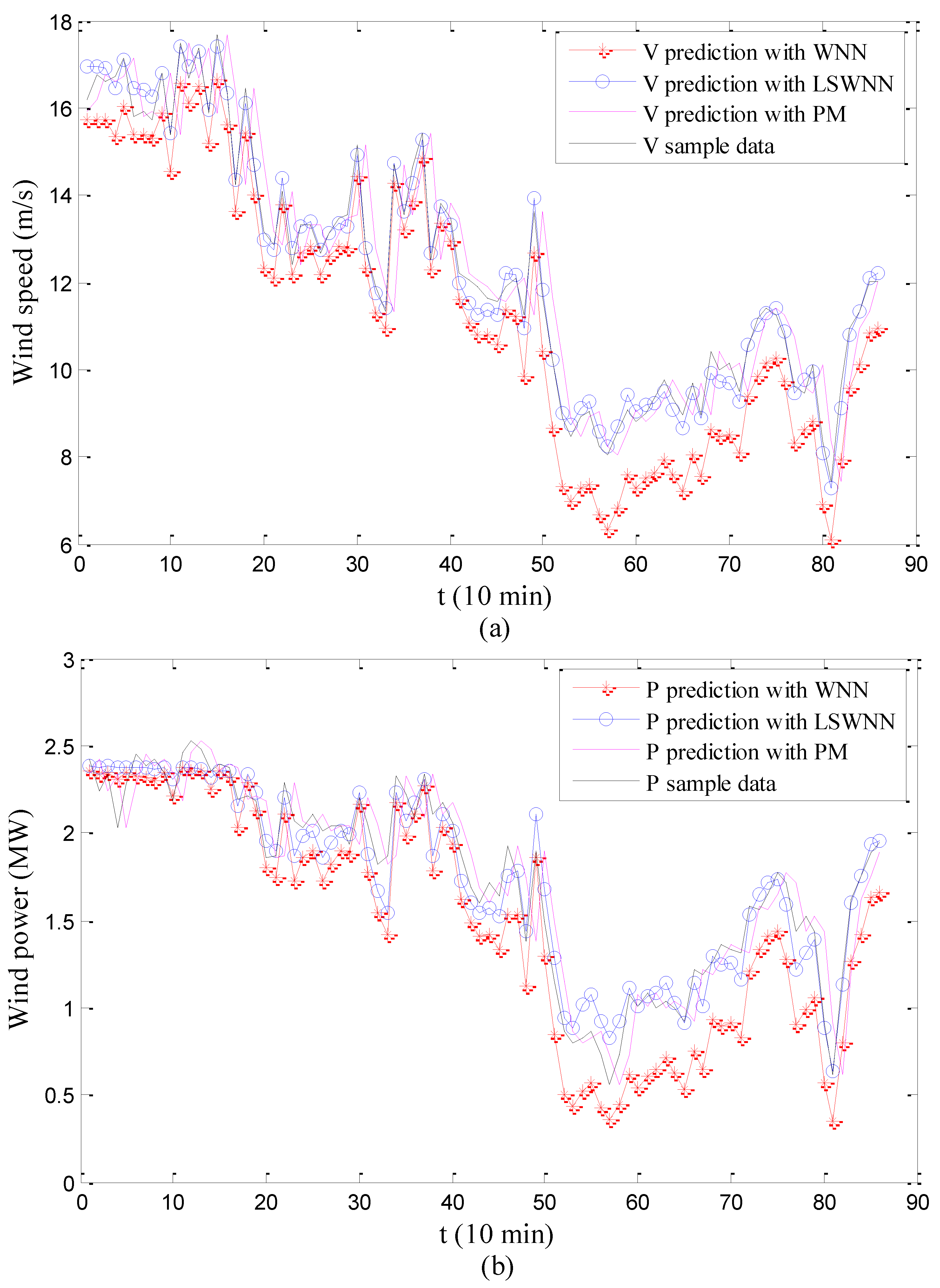
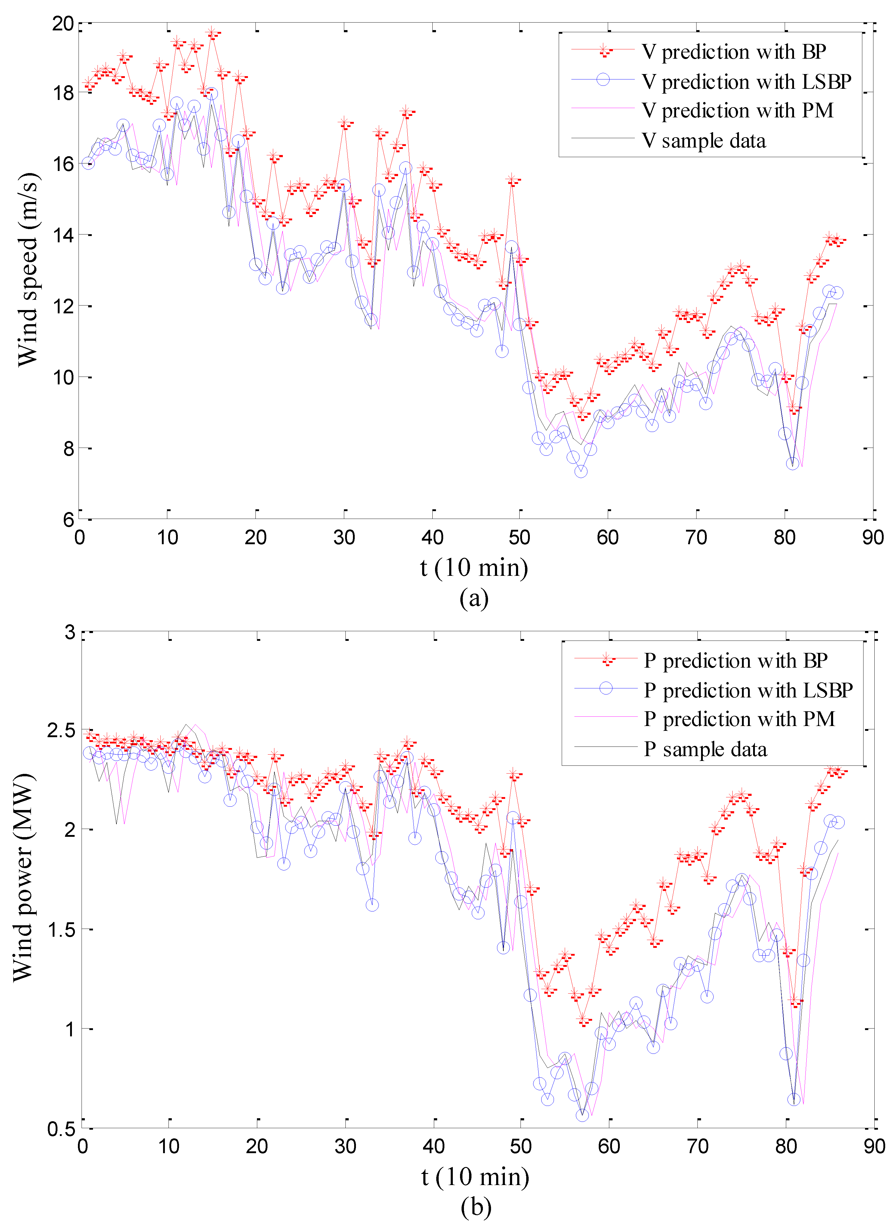
4. Wind Speed and Power Prediction Results and Error Analysis

In this paper, we analyze and evaluate the performance of various wind speed and power prediction models with the help of forecasting graphs and error statistics. We choose mean absolute error (MAE), mean squared error (MSE), and mean absolute percentage error (MAPE) as error indicators in this research. Error statistics of wind speed and power prediction in February 2014 are presented in Table 2 and Table 3. Formulas of these error criteria are given by:

$$MAE=\frac{1}{M}{\displaystyle \sum _{t=1}^M\left|y\left(t\right)-f\left(t\right)\right|}$$

(6)

$$MSE=\frac{1}{M}{\displaystyle \sum _{t=1}^M{\left(y\left(t\right)-f\left(t\right)\right)}^2}$$

(7)

$$MAPE=\frac{1}{M}{\displaystyle \sum _{t=1}^M\left|\frac{y\left(t\right)-f\left(t\right)}{y\left(t\right)}\right|}$$

(8)

wherein, y(t) and f(t) separately denote the observations and forecasts of wind speed or wind power at time t. M is sample size.

Table 2. MAE, MSE, and MAPE statistics of wind speed forecasting in the Sotavento wind farm in February 2014.

Wind speed prediction models (symbols)	Error
	MAE (m/s)	MSE (m2/s2)	MAPE (%)
WNN (Vf1)	1.0298	1.2635	9.4189
LSWNN (V1)	0.2123	0.0697	1.8209
BP (Vf2)	1.8030	3.3591	14.9113
LSBP (V2)	0.2902	0.1141	2.5353
SVM (Vf3)	0.6709	0.6751	5.5984
LSSVM (V3)	0.3778	0.2223	3.1729
PM	0.8694	1.2757	7.0925

Table 2. MAE, MSE, and MAPE statistics of wind speed forecasting in the Sotavento wind farm in February 2014.

Wind speed prediction models (symbols)	Error
	MAE (m/s)	MSE (m2/s2)	MAPE (%)
WNN (Vf1)	1.0298	1.2635	9.4189
LSWNN (V1)	0.2123	0.0697	1.8209
BP (Vf2)	1.8030	3.3591	14.9113
LSBP (V2)	0.2902	0.1141	2.5353
SVM (Vf3)	0.6709	0.6751	5.5984
LSSVM (V3)	0.3778	0.2223	3.1729
PM	0.8694	1.2757	7.0925

Table 3. MAE, MSE, and MAPE statistics of wind power forecasting in the Sotavento wind farm in February 2014.

Error	Wind power prediction models
	PM	WNN		BP		SVM
		Vf1	V1	Vf2	V2	Vf3	V3
MAE (MW)	0.1593	0.2476	0.0980	0.3147	0.0825	0.1475	0.0872
MSE (MW2)	0.0431	0.0819	0.0150	0.1320	0.0106	0.0309	0.0122
MAPE (%)	10.8252	18.3653	6.7683	24.3340	5.1664	9.7209	5.9801

Table 3. MAE, MSE, and MAPE statistics of wind power forecasting in the Sotavento wind farm in February 2014.

Error	Wind power prediction models
	PM	WNN		BP		SVM
		Vf1	V1	Vf2	V2	Vf3	V3
MAE (MW)	0.1593	0.2476	0.0980	0.3147	0.0825	0.1475	0.0872
MSE (MW2)	0.0431	0.0819	0.0150	0.1320	0.0106	0.0309	0.0122
MAPE (%)	10.8252	18.3653	6.7683	24.3340	5.1664	9.7209	5.9801

Table 2 shows that forecasting precisions of the three traditional models are greatly improved by the disturbance models. However, the LSWNN model has the best performance compared with any error indicator. The average error of the WNN model is reduced by 86% compared to the LSWNN model. The SVM model has better robustness than the BP and WNN networks. The LSSVM improvement is smaller than that of the other two models. The average error reduction of the SVM model is 50%. The initial wind speed forecasting errors of the BP model are worse than those of the other two models. However, the corrected results are much better than the LSSVM model. The average error reduction is about 88%, which is the largest improvement. Although the forecasting error of PM is better than the conventional WNN and BP models, it is much worse than the three disturbance models.

We take the wind speed sequences V and V_f as the input of wind power prediction models to verify the influence of atmospheric disturbance. All the comparison results are shown in Table 3. We can see that all of the improved wind speeds V achieve higher precision than V_f in wind power predictions. Compared with the result of V_f by WNN, BP and SVM, the average errors of V are reduced by 68%, 82% and 47%, respectively. Table 2 and Table 3 suggest that the performance of PM is much better than the conventional neural networks, except for SVM. However, the average errors of the three improved models in turn are reduced by 47%, 59% and 54% compared with PM. All of the above statistics prove the good properties and significance of applying Lorenz disturbances in wind speed and power forecasting.

Figure 4. (a) Wind speed forecasting graphs based on WNN, LSWNN, and PM; (b) Wind power forecasting graphs based on the output V and V_f of WNN, LSWNN, and PM.

Figure 4. (a) Wind speed forecasting graphs based on WNN, LSWNN, and PM; (b) Wind power forecasting graphs based on the output V and V_f of WNN, LSWNN, and PM.

Aside from error criteria, the forecasting graphs are also effective measurements to evaluate the performance of prediction models and results. Figure 4, Figure 5 and Figure 6 separately show the wind speed and power forecasting curves by various neural networks, PM, and improved wind disturbance models. The sample data of wind speed and power series are used as references. As we all know, the PM is very suitable for short-term wind forecasting. The forecasting curve of PM is used to determine + or – in the perturbation formula. As seen from Figure 4a, the forecasting curve by WNN model distributes lower than PM. Then we have to enhance the disturbance intensity to make the predicted result close to the actual one. On the contrary, in Figure 5a, the forecasting curve by the BP model distributes higher than PM so that the disturbance effect should be reduced. Figure 4a, Figure 5a and Figure 6a present a great improvement after introducing the Lorenz disturbance.

Figure 5. (a) Wind speed forecasting graphs based on BP, LSBP, and PM; (b) Wind power forecasting graphs based on the output V and V_f of BP, LSBP, and PM.

Figure 5. (a) Wind speed forecasting graphs based on BP, LSBP, and PM; (b) Wind power forecasting graphs based on the output V and V_f of BP, LSBP, and PM.

Figure 6. (a) Wind speed forecasting graphs based on SVM, LSSVM, and PM; (b) Wind power forecasting graphs based on the output V and V_f of SVM, LSSVM, and PM.

Figure 6. (a) Wind speed forecasting graphs based on SVM, LSSVM, and PM; (b) Wind power forecasting graphs based on the output V and V_f of SVM, LSSVM, and PM.

Then we continue to verify the effect of Lorenz disturbance on wind power forecasting. We separately use the original series V_f and the disturbed series V to do the wind power predictions. Figure 4b, Figure 5b and Figure 6b depict the corresponding wind power predictions. According to the statistics in Table 3 and the forecasting graphs in Figure 4b, Figure 5b and Figure 6b, the wind speed series which eliminate the nonlinear disturbance effect has a much better forecasting performance. This phenomenon applied to any forecasting models used in this study. The introduction of a nonlinear Lorenz disturbance actually exerts an important and positive impact on wind power prediction.

5. Conclusions

The atmospheric system is actually a complex nonlinear dynamic system, in which small changes of atmospheric state may lead to a dramatic variation on the subsequent atmospheric evolution. In this paper, we explore the impact of atmospheric perturbation on wind power forecasting by adopting a Lorenz system. In order to validate the feasibility and universality of the disturbance method, three different prediction models are applied in this research. As a result, it is feasible to introduce a Lorenz disturbance in wind power prediction, which could greatly improve the forecasting accuracy. Application of the perturbation method plays an extremely important role in wind power forecasting, to which more attention should be paid.

However, there are still some issues to be discussed. First, the value of the variable parameter $r$ is not determined. A chaotic Lorenz disturbance series can be obtained when $r$ is larger than 24.74. We have to establish a criterion to ensure the accurate selection of the values of $r$ according to different features of the sample wind data. Besides, in order to test the universality of the disturbance method, various prediction models and large amounts of sample data should be employed. It is promising to work out much more accurate wind forecasting results after introducing these refinements.

References

1. Global Wind Energy Council (GWEC). Available online: http://www.gwec.net/global-figures/graphs/ (accessed on 9 March 2014).
2. Hu, J.M.; Wang, J.Z.; Zeng, G.W. A hybrid forecasting approach applied to wind speed time series. Renew. Energy 2013, 60, 185–194. [Google Scholar] [CrossRef]
3. Zhang, W.Y.; Wang, J.J.; Wang, J.Z.; Zhao, Z.B.; Tian, M. Short-term wind speed forecasting based on a hybrid model. Appl. Soft. Comput. 2013, 13, 3225–3233. [Google Scholar] [CrossRef]
4. Wang, X.C.; Guo, P.; Huang, X.B. A review of wind power forecasting models. Energy Proced. 2011, 12, 770–778. [Google Scholar] [CrossRef]
5. Foley, A.M.; Leahy, P.G.; Marvuglia, A.; Mckeogh, E.J. Current methods and advances in forecasting of wind power generation. Renew. Energy 2011, 37, 1–8. [Google Scholar] [CrossRef] [Green Version]
6. Chen, Z.H.; Xu, Y.; Xu, P.H.; Yang, H.Q.; Xiong, S.Q. Principle of Wind Power Prediction Technology and Business Systems, 1st ed.; China Meteorological Press: Beijing, China, 2013; pp. 18–41. [Google Scholar]
7. Bouzgou, H.; Benoudjit, N. Multiple architecture system for wind speed prediction. Appl. Energy 2011, 88, 2463–2471. [Google Scholar] [CrossRef]
8. Yesilbudak, M.; Sagiroglu, S.; Colak, I. A new approach to very short term wind speed prediction using k-nearest neighbor classification. Energy Convers. Manag. 2013, 69, 77–86. [Google Scholar] [CrossRef]
9. Liu, H.; Tian, H.Q.; Chen, C.; Li, Y.F. A hybrid statistical method to predict wind speed and wind power. Renew. Energy 2010, 35, 1857–1861. [Google Scholar] [CrossRef]
10. Tascikaraoglu, A.; Uzunoglu, M. A review of combined approaches for prediction of short-term wind speed and power. Renew. Sustain. Energy Rev. 2014, 34, 243–254. [Google Scholar] [CrossRef]
11. Gan, M.; Ding, M.; Huang, Y.Z.; Dong, X.P. The effect of different state sizes on Mycielski approach for wind speed prediction. J. Wind Eng. Ind. Aerodyn. 2012, 109, 89–93. [Google Scholar] [CrossRef]
12. Martinez-Morales, J.D.; Palacios, E.; Velazquez-Carrillo, G.A. Wavelet neural networks for predicting engine emissions. Proced. Technol. 2013, 7, 328–335. [Google Scholar] [CrossRef]
13. Zhou, J.Y.; Shi, J.; Li, G. Fine tuning support vector machines for short-term wind speed forecasting. Energy Convers. Manag. 2011, 52, 1990–1998. [Google Scholar] [CrossRef]
14. Monfared, M.; Rastegar, H.; Kojabadi, H.M. A new strategy for wind speed forecasting using artificial intelligent methods. Renew. Energy 2008, 34, 845–848. [Google Scholar] [CrossRef]
15. Liu, H.; Tian, H.Q.; Li, Y.F. Comparison of two new ARIMA-ANN and ARIMA-Kalman hybrid methods for wind speed prediction. Appl. Energy 2010, 98, 415–424. [Google Scholar] [CrossRef]
16. Sheela, K.G.; Deepa, S.N. Neural network based hybrid computing model for wind speed prediction. Neurocomputing 2013, 122, 425–429. [Google Scholar] [CrossRef]
17. Liu, H.; Tian, H.Q.; Pan, D.F.; Li, Y.F. Forecasting models for wind speed using wavelet, wavelet packet, time series and artificial neural networks. Appl. Energy 2013, 107, 191–208. [Google Scholar] [CrossRef]
18. Zhang, Y.; Wang, J.X.; Wang, X.F. Review on probabilistic forecasting of wind power generation. Renew. Sustain. Energy Rev. 2014, 32, 255–270. [Google Scholar] [CrossRef]
19. Guo, Z.H.; Chi, D.Z.; Wu, J.; Zhang, W.Y. A new wind speed forecasting strategy based on the chaotic time series modelling technique and the Apriori algorithm. Energy Convers. Manag. 2014, 84, 140–151. [Google Scholar] [CrossRef]
20. Zhang, Y.G.; Yang, J.Y.; Wang, K.C.; Wang, Y.D. Lorenz wind disturbance model based on grey generated components. Energies 2014, 7, 7178–7193. [Google Scholar] [CrossRef]
21. Liu, B.Z.; Peng, J.H. Nonlinear Dynamics, 1st ed.; Higher Education Press: Beijing, China, 2007; pp. 120–143. [Google Scholar]
22. Lorenz, E.N. The Butterfly Effect; Premio Felice Pietro Chisesi e Caterina Tomassoni award lecture; University of Rome: Rome, Italy, 2008. [Google Scholar]
23. Lorenz, E.N. Deterministic nonperiodic flow. J. Atmos. Sci. 1963, 20, 130–141. [Google Scholar] [CrossRef]
24. Algaba, A.; Fernandez-Sanchez, F.; Merino, M.; Rodriguez-Luis, A.J. Comments on ‘Global dynamics of the generalized Lorenz systems having invariant algebraic surfaces’. Phys. D Nonlinear Phenom. 2014, 266, 80–82. [Google Scholar] [CrossRef]
25. Moghtadaei, M.; Hashemi Golpayegani, M.R. Complex dynamic behaviors of the complex Lorenz system. Sci. Iran. D 2012, 19, 733–738. [Google Scholar] [CrossRef]
26. Lorenz, E.N. The Essence of Chaos, 1st ed.; China Meteorological Press: Beijing, China, 1997; pp. 127–137. [Google Scholar]
27. Saltzman, B. Finite amplitude free convection as an initial value problem-I. J. Atmos. Sci. 1962, 19, 329–341. [Google Scholar] [CrossRef]