1. Introduction
Wind turbines (WT) are influenced strongly by the atmosphere’s natural variability, including thermal stratification and wind conditions. In fact, the surrounding turbulent atmospheric boundary-layer structure significantly impacts the turbulent wakes generated by the WT. When deployed as large arrays in wind farms, fatigue, power losses and reduced life expectancy are caused by the wakes generated by the turbines and their potential interactions with neighboring turbines. Such issues have created a bottleneck, limiting wind power as an accessible source of renewable energy. Turbulence generated by the rotating turbine rotors interacts with the turbulent ABL, resulting in a highly mixed region behind the wind turbine, which spans several turbine diameters downstream of the WT [
1,
2]. Streamwise and transverse transport of momentum by turbulence results in horizontal wake expansion [
3]. Consequently, downstream WTs encounter the wake turbulence of the upstream WTs. Knowledge of turbulence and flow conditions in the wake region of the upstream WTs are essential for realistically predicting the power output, fatigue, and life cycle of the WTs placed behind the originals [
4,
5,
6]. Moreover, when the WTs are in a cluster, ABL-induced wake effects lead to wake-wake interactions between neighboring WTs, resulting in enhanced turbulence over the entire wind farm. In fact, research has demonstrated that wake interactions between turbines are important aerodynamic factors affecting the overall performance of wind farms [
5].
Unfortunately, the interaction of ABL turbulence with wind turbine wakes is poorly understood due to the complex structure of ABL. Stable ABL regimes are present when the underlying land surface is cooler than the air above, such as during the nighttime. Field measurements from the Cooperative Atmospheric-Surface Exchange Study 99 (CASES-99) have clearly demonstrated the presence of jet-like structures known as low-level jets (LLJs) in the nocturnal boundary-layer [
7]. In stable ABL, turbulence is the resultant balance between turbulence shear generation and damping due to buoyancy. Increasing stability results in shallower ABL with lower turbulence. Further, it reduces the downward momentum transfer from the top of the ABL [
8]. Stable ABL is topped by the LLJs [
8]; strong shear due to LLJ and the vertical transport of momentum towards the surface enhances the turbulence and mixing in the boundary layer [
9,
10].
Experimental and numerical studies have revealed that WT wake structure is complicated. Strong swirling motions have been observed in the near-wake region resulting in the wake’s rotational structure. Recent studies have demonstrated strong counter-rotating (opposite to rotor rotation) downstream wakes [
11,
12]. The WT wake region is defined by a combination of spiraling tip vortices from the blades of the WT—which follow a helical path—and the corresponding root vortices. To date, the vortex behavior in the wake region remains unclear. Idealized models have observed the root vortices to be unstable, and hence, ceasing to exist beyond 3
D downstream distance (where
D is rotor diameter), whereas tip vortices persist far into the wake [
2]. Meanwhile, research has shown the helical structure of the tip vortices to be unstable to small perturbations [
13]. Experimental visualizations of Felli, Camussi, and Di Felice [
14] and Sherry
et al. [
15], as well as the numerical simulations of Sorensen and Shen [
16] and Ivanell
et al. [
13] have shown that tip vortices undergo pairing which results in the merging of vortices. Windnall [
17] has hypothesized vortex merging to be one of the modes of instability of a helical vortex filament, appearing as the pitch of the helix decreases and resulting in the interaction of neighboring filaments. Adding complexity to the wake structure, Medici and Alfredsson have observed an additional low-frequency wake instability resulting in meandering motions of the wake [
18]. More recently, Kang, Yang, and Sotiropoulos [
19] attributed the lateral meandering of the wake to the interaction of the spiraling hub vortex with the shear layer. However, these studies have been limited to idealistic wind conditions where the wake structure is symmetric and the wind shear and wind angle are assumed to be constant. In reality, height-dependent wind characteristics influence the wake quite differently.
The significance of atmospheric stability is gaining recognition with recent efforts focused on realistic flow conditions. Bhaganagar and Debnath [
20] isolated the role of low-level jets (LLJ) on the turbulence developed in wind turbine wake. This study is promising as it is one of the first to rigorously demonstrate the influence of large-scale mean forcings, including LLJs, on the turbine wake structure. It revealed that, in addition to shear-generated turbulence from the tip and root vortices, other factors produce turbulence, including interactions between root and tip vortex and vortex merging. Using an experimental wind tunnel facility on scaled WTs, Hu, Yang, and Sarkar [
21] demonstrated that dynamic loading on wind turbines is a factor higher for realistic conditions than uniform flow conditions. Using the weather model, Mirocha
et al. [
22] demonstrate the enhanced turbulence caused by realistic atmospheric conditions. This study represents the first time atmospheric turbulence and WT wake interactions have been pursued, a critical step towards predicting accurate wind turbine life cycle and fatigue.
The current research is a fundamental study undertaken to address a critical need in the wind turbine industry: to numerically simulate WT wakes subjected to a realistic ABL environment using large-eddy-simulations. Our work is an important contribution, providing one of the first detailed wake structures due to ABL and WT interactions. We limit our study to stable nighttime ABL conditions. The manuscript has two primary focuses: to understand the turbines’ turbulent wake structure and to determine the ABL metrics that influence the turbine wake.
Our primary question is as follows: How do the metrics of the ABL—stability, wind direction, wind shear and turbulence-affect the wind turbines’ wake structure? We conducted our analysis for WT subjected to ABL under low- and moderately—stable regimes and simulated two distinct idealized ABL regimes in order to understand how atmospheric structures influenced the wake of the wind turbines. The low-stable ABL regime is similar to the one described in Kosovic and Curry [
23], imposing a steady surface-cooling rate of −0.25 K/h. and a surface temperature of 263 K. The conditions selected by Kosovic and Curry [
23] matched the Beaufort Sea Arctic Stratus Experiment (BASE), resembling a clear-air stable ABL driven by a low surface cooling rate. We imposed a moderate surface cooling rate of −1.0 K/h. and a surface temperature of 256 K to generate a moderately stable ABL regime. As Zhou and Chow [
24] demonstrated, a surface cooling rate up to −1.25 K/h. generates continuous turbulence without intermittency, with the LLJ occurring at a height of 80–100 m. The low-state ABL regime corresponds to a deeper ABL with stronger and continuous turbulence where the LLJs occur at a height of 180–200 m and surface temperature of 263 K. The peak LLJ velocity is 10 m/s. The moderately stable ABL regime corresponds to a shallower ABL, but one that is still in a continuous turbulent state where LLJs move closer to the surface and occur at a height of 80–100 m with a peak velocity of 12 m/s and surface temperature of 256 K.
2. Large Eddy Simulation (LES) and Validation
The LES tool used in this study is similar to code used [
25,
26] and validated for stable ABL by Bhaganagar and Debnath [
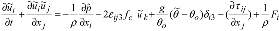
20]. For sake of continuity the details are repeated. The governing equations used are the filtered Navier-Stokes equations (momentum and potential temperature transport Equations) with Boussinesq approximation as follows:
where, a tilde denotes the spatially resolved filtered component at scale ∆,
![]()
denotes the modified pressure. The spatial gradient of the mean pressure term acts to drive the flow convection, (
u1,
u2,
u3) = (
u,
v,
w) are the components of the velocity field (
u is the axial component;
v is the lateral or
y-component; and
w is the vertical component).
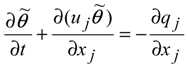
![]()
is the resolved potential temperature; θ
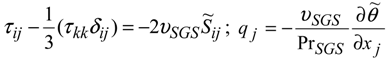
0 is the reference temperature. The subgrid stresses (SGS) are included in the τ term along with the fluid stress tensor. The SGS flux and SFS temperature flux are parameterized, respectively as follows:
where D is the deviatoric SGS stress tensor;
vSGS is the SGS eddy viscosity; and Pr
SGS is the SGS Prandtl number. The SGS flux is computed using the Moeng’s model [
27] which is an improvement over the Smagorinsky model, where the turbulent viscosity and turbulent kinetic energy are modeled as follows:
![]()
and
![]()
, Δ = (Δ
xΔ
yΔ
z)
1/3 using the mesh cells in x, y and z directions, the resolved strain-rate tensor is, and Pr
SGS is constant (ref dependent on stratification level).
The Coriolis parameter is defined as fc = 2ω[0,cos(φ),sin(φ)]; φ is the latitude; and ɷ is the planetary rotation rate. The last term Fi in the momentum equation is the wind-turbine induced forces generated by the actuator line model.
Wall models are specified for the surface shear stress and surface heat flux. The surface shear stress model is that of Schumann [
28]. At the surface, the stress tensor components are zero expect for τ
13 and τ
23. They are specified as:
where, u
τ is the friction velocity; z
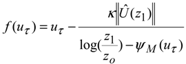
1 denotes the height of the center of the cells adjacent to the wall, brackets denote horizontal average. The friction velocity is determined by solving the Monin-Obukhov scaling, which is an implicit function of u
τ given as follows:
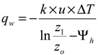
Similarly, the surface heat flux (
qw) is specified as follows:
where κ is the von-Karman constant; z
o is the aerodynamic roughness height; and ψ
M and ψ
H are the stability parameters that are functions of various quantities including μ
τ.
For stable ABL simulation, we specify the surface cooling rate and the surface heat flux is determined using the Monin-Obhukov scaling laws for velocity and potential temperature, which account for the difference between surface temperature and temperature at cell center adjacent to the wall. At each time step, the surface temperature flux is specified uniformly over the lower surface similar to work of Basu
et al. [
29].
Table 1 shows the validation of the LES model with LES inter-comparison study [
23] and study of Basu
et al. [
29].
Table 1.
Grid convergence of surface buoyancy flux, surface momentum flux, ABL height (Hδ), Richardson’s number at hub-height (Ri (hub)) and friction velocity (uτ) conducted with grid spacing of 3.125 m and 6.25 m.
Table 1.
Grid convergence of surface buoyancy flux, surface momentum flux, ABL height (Hδ), Richardson’s number at hub-height (Ri (hub)) and friction velocity (uτ) conducted with grid spacing of 3.125 m and 6.25 m.
Low Stratification
(Validation) | Cs × ∆ (m) | Surface Buoyancy
Flux (K-m/s) | Surface Momentum Flux (m2/s2) | Hδ (m) | Ri (hub) | uτ (m/s) |
|---|
| ∆ = 6.25 m | 0.1 × 6.25 | −4.2 × 10⁻⁴ | 0.068 | 162.5 | 0.17 | 0.24 |
| ∆ = 3.125 m | 0.132 × 3.125 | −3.2 × 10⁻⁴ | 0.058 | 156 | 0.169 | 0.22 |
| Inter-comparison study [23] | Dynamic × (1–6.25) | 3.5–5.5 × 10⁻⁴ | 0.06–0.08 | 158–211 | - | 0.22–0.28 |
| Basu
et al. [29] | Dynamic × (3.31–6.25) | −4.0–4.7 × 10⁻⁴ | 0.068–0.076 | 173–187 | 0.17 | 0.26–274 |
Mesh refinements have been performed by refining the wake region with a grid size of 1 m. The time step used for the simulation is 0.5 s. At initialization, we applied a random perturbation of 0.1 K to the bottom 100 m of the domain to trigger turbulence. Simulations are carried out for a total of 40,000 s (refer to Bhaganagar and Debnath [
20] for validations of the stable ABL simulations).
Following the work of Sorensen and Shen [
16], the rotor is approximated using an actuator line model (ALM), where the force field generated by the rotor is approximated as a body force term in the momentum equation. The individual blade loads are modeled through a suitable distribution of body forces along the blade, with strengths determined from inflow conditions. We used a Gaussian-shaped projection function to project body forces on a finite volume surrounding the actuator line while preventing numerical instabilities. Similar methodology has been used successfully by Lu and Porte-Agel [
30]. The root and tip vortices are captured well. Based on the recommendation of Zahle and Sorensen [
31], we have used fine resolution in the wake region, up to 10 rotor diameters, in order to accurately capture the near-wake vortex structures.
The stable ABL simulations have been performed for the following conditions: (a) south-east Kansas night-time conditions during the month of October based on CASES-99 field experiment with surface temperature in range of (275 K–287 K) [
7]; (b) wind turbine locations at sweet-water, Texas with surface temperature in range of (288 K–293 K) [
32]; (c) arctic stratus base experiments (256 K–269 K) [
23]. The conclusions from these simulations is that low-level jets exist in stable ABL, with increasing surface temperature the height of LLJ increases for a given surface cooling rate. Increasing the cooling rate lowers the LLJ height. Further, we observed that with higher surface temperatures, the time to reach equilibrium state increases; hence care has to be taken to monitor surface heat-flux, surface buoyancy-flux and LLJ height for the simulation to reach a statistical equilibrium state.
3. Structure of Atmospheric Boundary Layer: ABL Metrics of Relevance to WT Wakes
Low- and moderate-stability ABL regimes were generated by simulating the precursor ABL for 40,000 s. The statistics were computed when ABL reached a quasi-equilibrium state, which is defined as the state of ABL when there were relatively fewer changes in the height of that layer, the surface fluxes of momentum, and heat change with time. Thus ensuring turbulence is in an equilibrium state.
Table 2 specifies the ABL parameters for both the cases that are considered in the present study.
Table 2.
ABL parameters cooling rate, surface temperature, heat flux, friction velocity, Monin-Obhukov (MOB) length (L) and Richardson number at hub height for low and moderate stratified cases.
Table 2.
ABL parameters cooling rate, surface temperature, heat flux, friction velocity, Monin-Obhukov (MOB) length (L) and Richardson number at hub height for low and moderate stratified cases.
Case
(Stratification) | Cooling rate
(K/h) | Surface temperature (K) | Heat flux
(K·m/s) | Friction velocity (m/s) | MOB length L (m) | Ri (hub) |
|---|
| Low | −0.25 | 263.1 | 0.012 | 0.22 | 82 | 0.17 |
| Moderate | −1.0 | 257.3 | 0.02 | 0.175 | 24 | 0.22 |
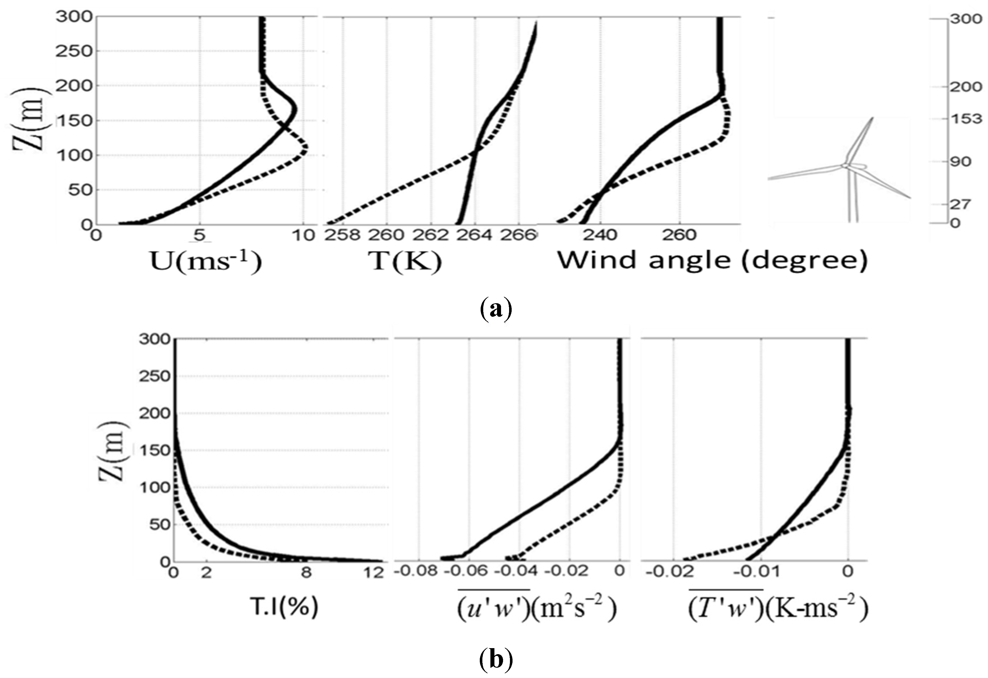
Profiles of time-averaged streamwise velocity (
U), temperature (
T), and wind angle are shown in
Figure 1. The relative position of the WT also is shown in the figure. The hub-height of the WT is 90 m and the rotor diameter is 126 m. The lower tip of the blade is at 27 m and the upper tip of the blade is at 153 m. For the low-stability ABL regime, LLJs with a peak velocity of 9.5 m/s occur between
z is 150–200 m. In comparison, the LLJs occur much lower in height and with a higher peak velocity of 10 m/s for the moderate-stability ABL regime. This finding is consistent with field observations that increasing atmospheric stability increases the LLJ strength and decreases the height of their occurrence.
It is interesting to note that the wind angle changes with height and also with atmospheric stability. The wind angle changes significantly across the atmospheric boundary height and reaches a geostrophic condition of 270 wind angles at the edge of the ABL (west facing wind). At the surface, the higher the atmospheric stability, the higher is the wind angle. As expected, the height variation in the wind angle for the moderate stability ABL regime stable is more drastic.
Figure 1.
ABL metrics that are of significant to WT wake dynamics: (a) mean streamwise velocity, mean temperature and wind angle (degrees); (b) turbulence intensity (T.I.), shear stress and buoyancy flux. Solid line represents the low-stable ABL regime and the dashed line represents the moderately-stable ABL regime.
Figure 1 also shows the variation of root-mean-square of streamwise velocity fluctuations, Reynolds shear stress, and buoyancy flux with height (
Figure 1b). Increasing atmospheric stability lowers the turbulence intensity and Reynolds stresses, whereas it increases the buoyancy flux. Due to the shear and turbulence damping by the buoyancy, the depth of the stable boundary layer is dictated by the turbulence production. Increasing stability lowers the depth of the stable boundary layer due to increased buoyancy-induced damping.
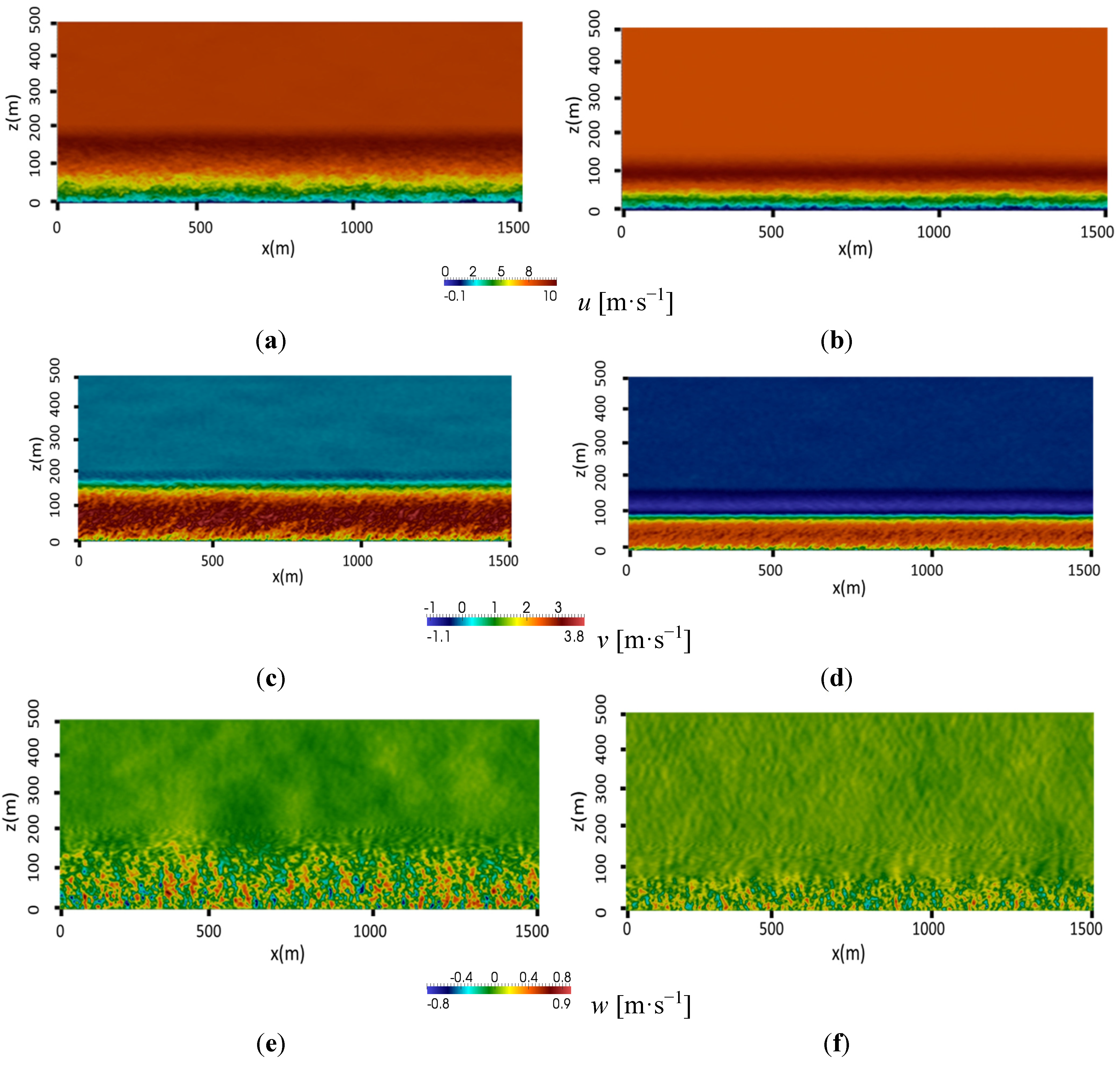
We next present the structure of the instantaneous velocity in the
x-z plane in
Figure 2.
Figure 2a,b show the streamwise (
u) structures for the low- and moderate-stability regimes, respectively. The corresponding spanwise (
v) and wall normal (
w) structures for the two regimes are shown in
Figure 2c–e. Dominant LLJs marking the edge of the boundary layer are seen clearly in the velocity structures. The
u structures are significantly large-scale motions. Regions of high shear are present close to the surface and near the LLJs due to strong velocity gradients for both the low- and moderate-stability regimes. However, as the LLJs move closer to the surface with increasing stability, the resultant wind shear increases greatly for the higher-stability ABL regime. The
v structures are also significantly dominant and characterized by large-scale motions similar to the
u structures. The
w structures are oriented predominantly in the vertical direction. It is important to note that, for ABL flows, the horizontal pressure gradient is a balance of the Coriolis force and Reynolds stresses (from the momentum Equations).
Figure 2.
Structure in the x-z plane of instantaneous (a) streamwise velocity for low-stability; (b) streamwise velocity for moderate-stability; and (c) spanwise velocity for low-stability; (d) spanwise velocity for moderate-stability; (e) wall-normal velocity for low-stability; (f) wall-normal velocity for moderate-stability ABL regimes.
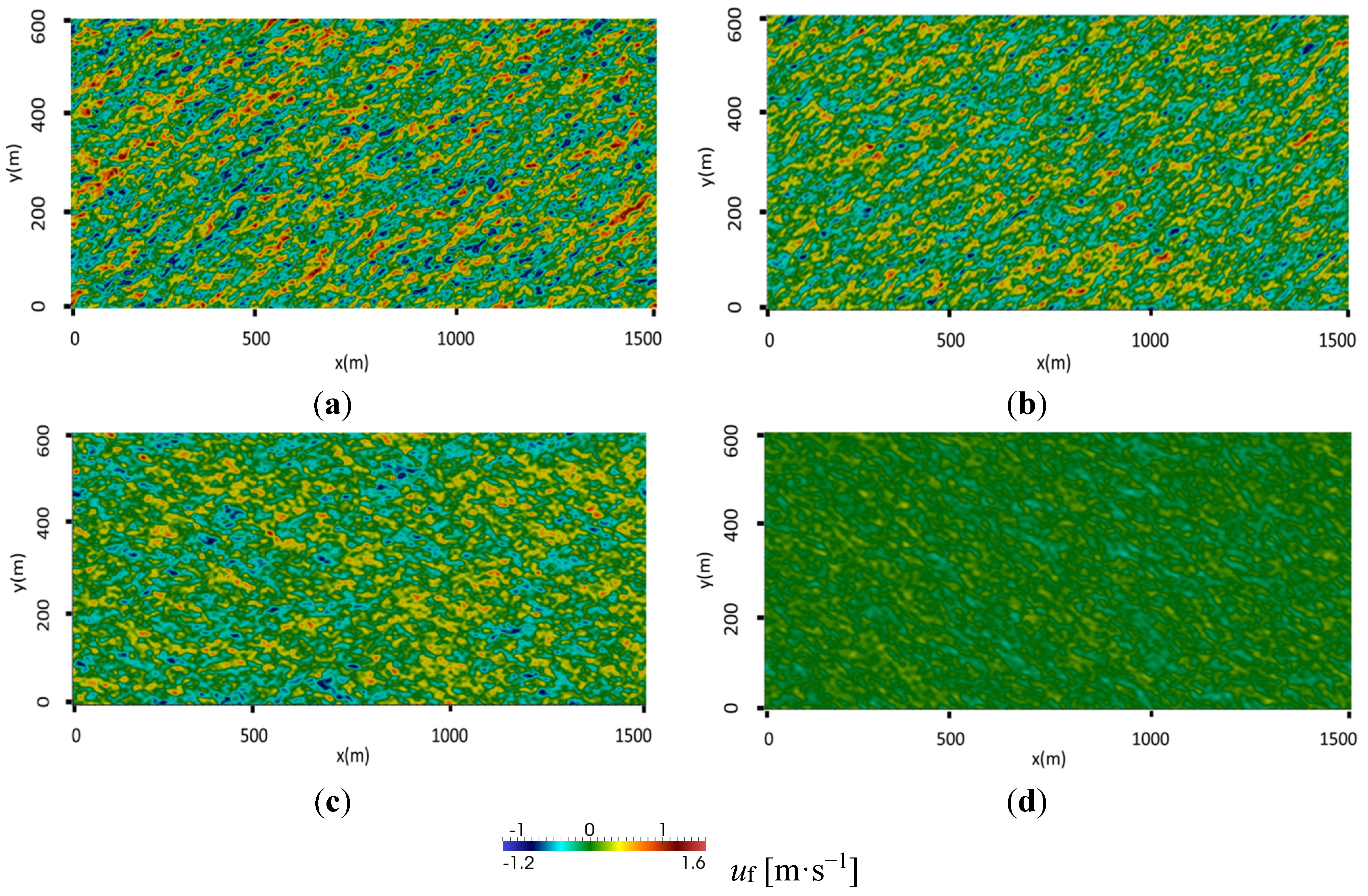
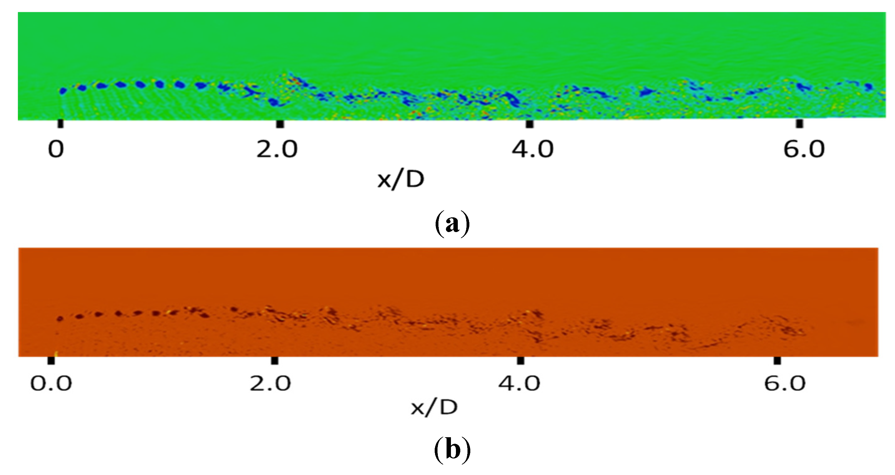
Figure 3 shows the streamwise velocity fluctuations (time-averaged streamwise velocity subtracted from the instantaneous streamwise velocity), which represent the streaks in the horizontal plane at various heights above the surface.
Figure 3a,b show the streaks at height
z = 30 m above the surface for low- and moderate-stability cases, respectively. At this height, the streamwise streak spacing is much smaller for the low-stability regime than for the moderate-stability regime, thus indicating higher turbulence for the low-stability regime. The streaks at
z = 90 m (hub-height) are presented in
Figure 3c and
Figure 3d for low- and moderate-stability ABL regimes, respectively. As expected with increasing height, turbulence decreases for both regimes. At the hub-height, the turbulence for the low-stability regime is still strong, whereas turbulence practically has vanished for the moderate-stability regime, as the LLJs occur around this height, which corresponds to the edge of the ABL.
Figure 3.
Streamwise fluctuating velocity (uf) (a) low-stable at z = 30 m; (b) moderate-stability at z = 30 m; (c) low-stability at z = 90 m; (d) moderate-stability at z = 90 m (hub-height) ABL regimes.
Figure 3.
Streamwise fluctuating velocity (uf) (a) low-stable at z = 30 m; (b) moderate-stability at z = 30 m; (c) low-stability at z = 90 m; (d) moderate-stability at z = 90 m (hub-height) ABL regimes.
In summary, turbulence structures are significantly different between the ABL under low- and moderate-stability regimes, and these differences are of significant consequence to WT wake evolution and dynamics. With increasing stability, the LLJs move towards the surface, resulting in a shallower boundary layer. The resultant turbulence kinetic energy in the ABL results from the balance of turbulence shear production and buoyancy damping. The wind shear governs the resultant turbulence shear production in the ABL; however, the mean temperature gradient and the buoyancy flux govern the net turbulence damping. The variation of the wind angle with height not only changes the wind shear, but also the Reynolds stresses and buoyancy flux with height. Wind shear, wind angle, mean temperature gradient, Reynolds stresses, and buoyancy flux, T'w' are the ABL metrics that are strongly dependent on atmospheric stability for stable ABL, which plays an important role in dictating the near-wake dynamics of WT.
4. Interactions of Atmospheric Boundary Layer and Wind Turbines
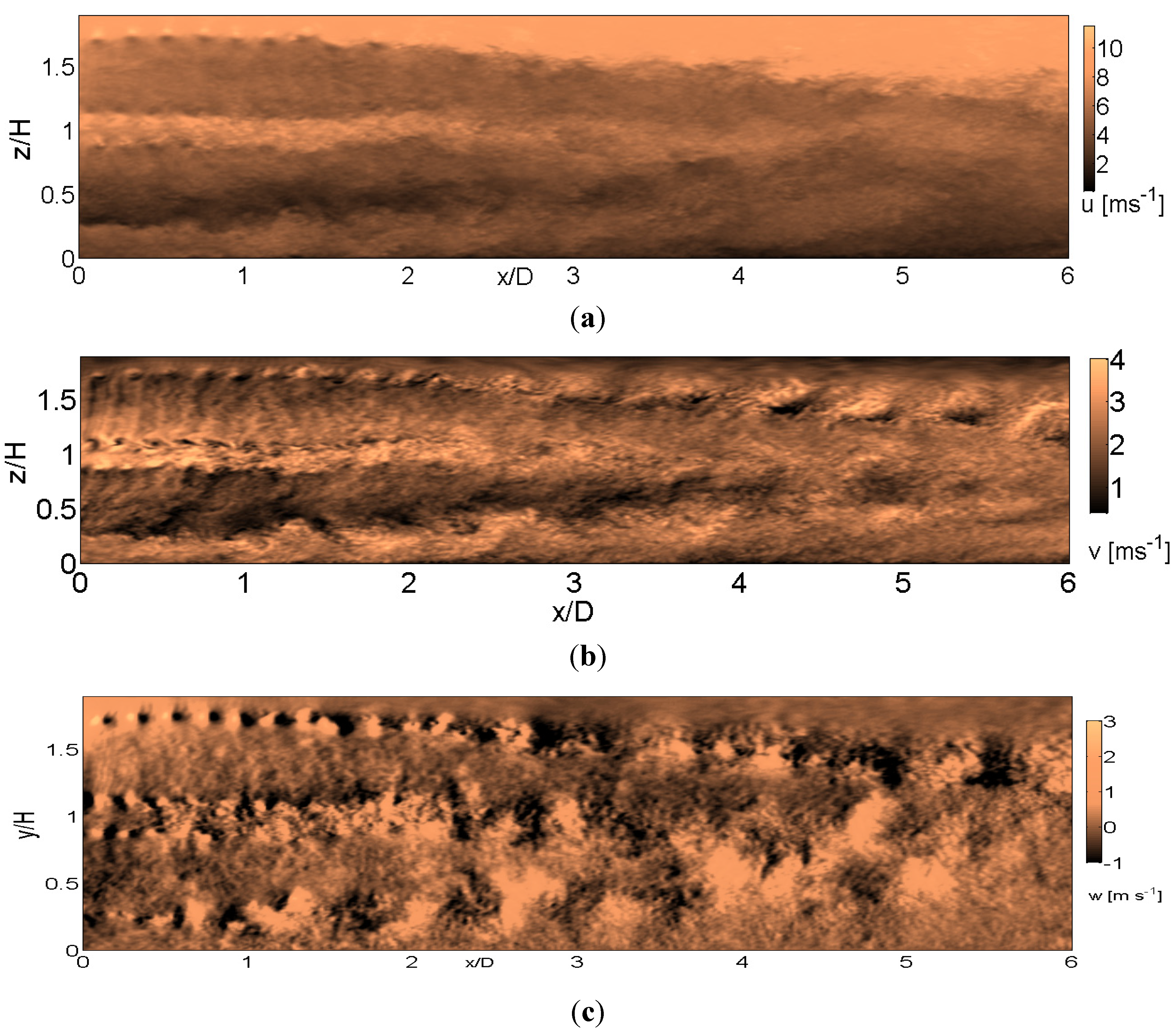
After performing the initial precursor ABL simulations for 50,000 s, the final state of ABL is used as the initial condition for the WT simulations. It should be noted that, in addition to ABL mean flow, the state of ABL turbulence also needs to be introduced in the WT simulations by accurately representing all the components of Reynolds stresses, turbulence mixing coefficients, and heat flux coefficients. The WT simulations are performed for 200 s with boundary conditions and surface cooling rates identical to the ABL simulations. The simulations are performed with a much-refined grid spacing of 0.75 m to resolve the wake structure. The statistics are averaged for the last 100 s after the initial transience passes.
4.1. Wake Structure of Wind Turbine in a Low-Stable ABL Regime
We present streamwise (
u), spanwise (
v), and wall-normal (
w) velocity structures in
Figure 4. The large-scale features of the wake structure are clearly evident. LLJ observed in the ABL at a height of 2
H persist in the near-wake region as well.
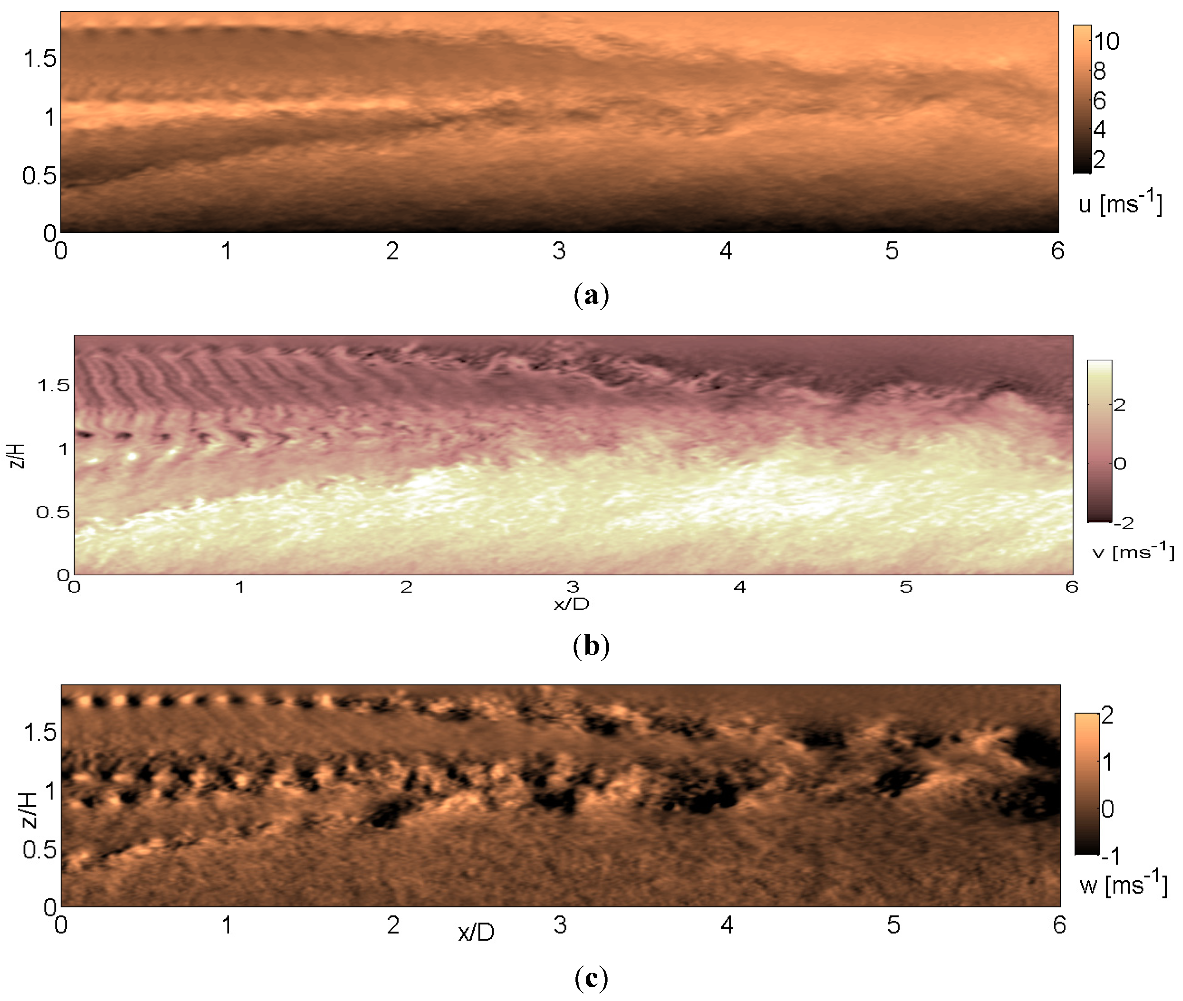
Figure 4.
Velocity structure of the (a) streamwise velocity; (b) spanwise velocity; (c) wall-normal velocity, at the center plane, y/D = 0 for WT in low-stable ABL regime.
Figure 4.
Velocity structure of the (a) streamwise velocity; (b) spanwise velocity; (c) wall-normal velocity, at the center plane, y/D = 0 for WT in low-stable ABL regime.
We present streamwise (
u), spanwise (
v), and wall-normal (
w) velocity structures in
Figure 4. The large-scale features of the wake structure are clearly evident. LLJ observed in the ABL at a height of 2
H persist in the near-wake region as well.
Figure 4a shows distinct tip vortices at the blade tips (
z = 0.2
H &
z = 1.7
H) and root vortices at the hub-height in the
u velocity contours. Similar helical tip vortices and root vortices have been revealed in the particle image velocimetry (PIV) measurements [
33,
34] and the hot-wire anemometer measurements [
35,
36]. Strong shear layer is generated at the lower tip, which interacts with root vortex in the region of
x/D = 2–3 (striking location varies depending on the
y location). The root vortex follows a linear trajectory to
x = 0.9
D and beyond, meandering in the
y–z plane. Significant mixing initiates from
x/D = 2 in the region between the blade tips. The spanwise- structures are characterized by alternate positive and negative values, which are signatures of the tip vortex up to
x/D= 2.0 (
Figure 4b). Large-scale, well-defined coherent motions are evident further downstream, indicating large-scale mixing. Similar coherent patterns have been observed in turbulent mixing layers. As pockets of clear large-scale entrainment at the upper-blade tip become evident due to coherent mixing, the vertical structures show significant change in flow characteristics from
x/D = 2 (
Figure 4c).
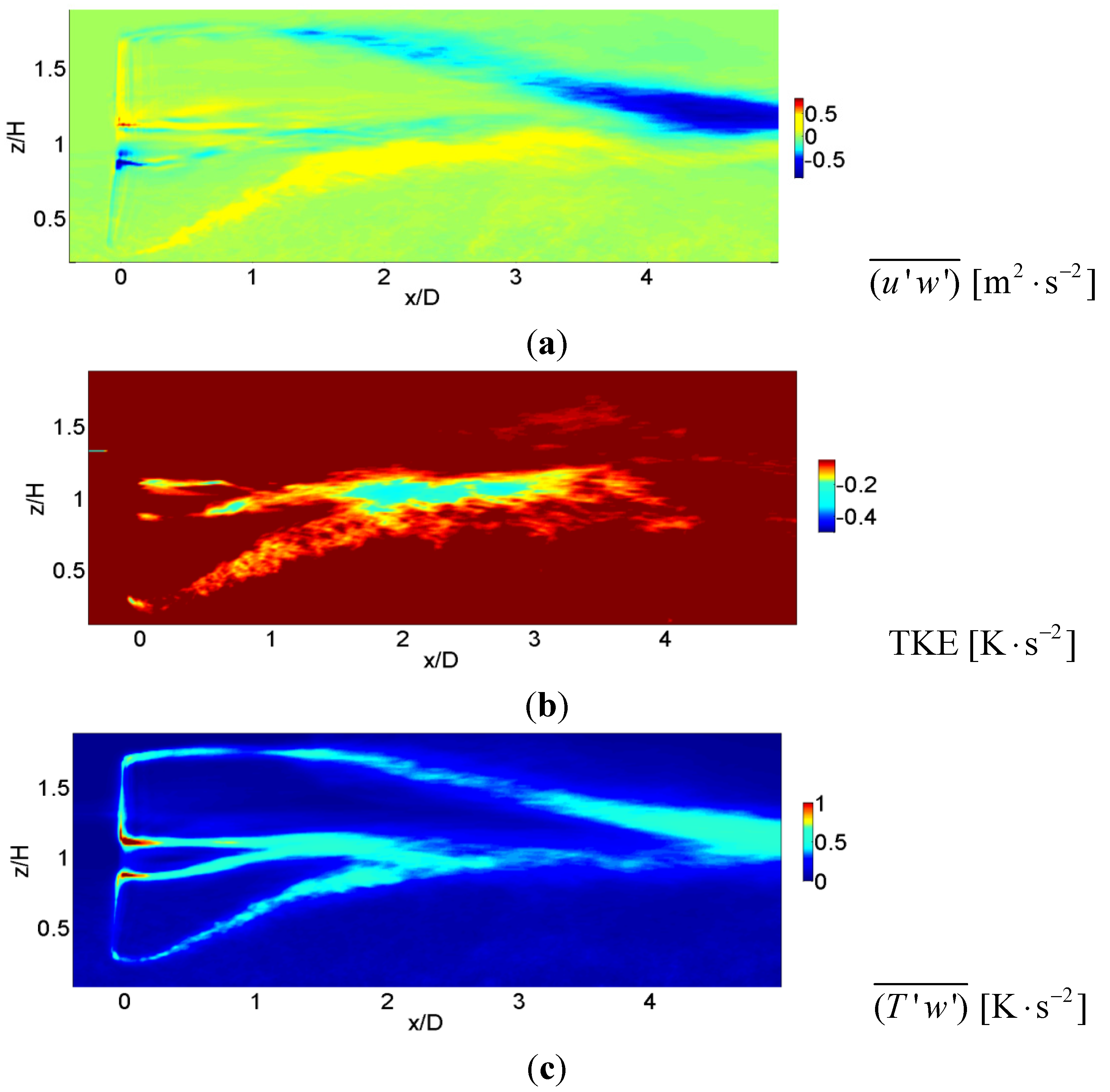
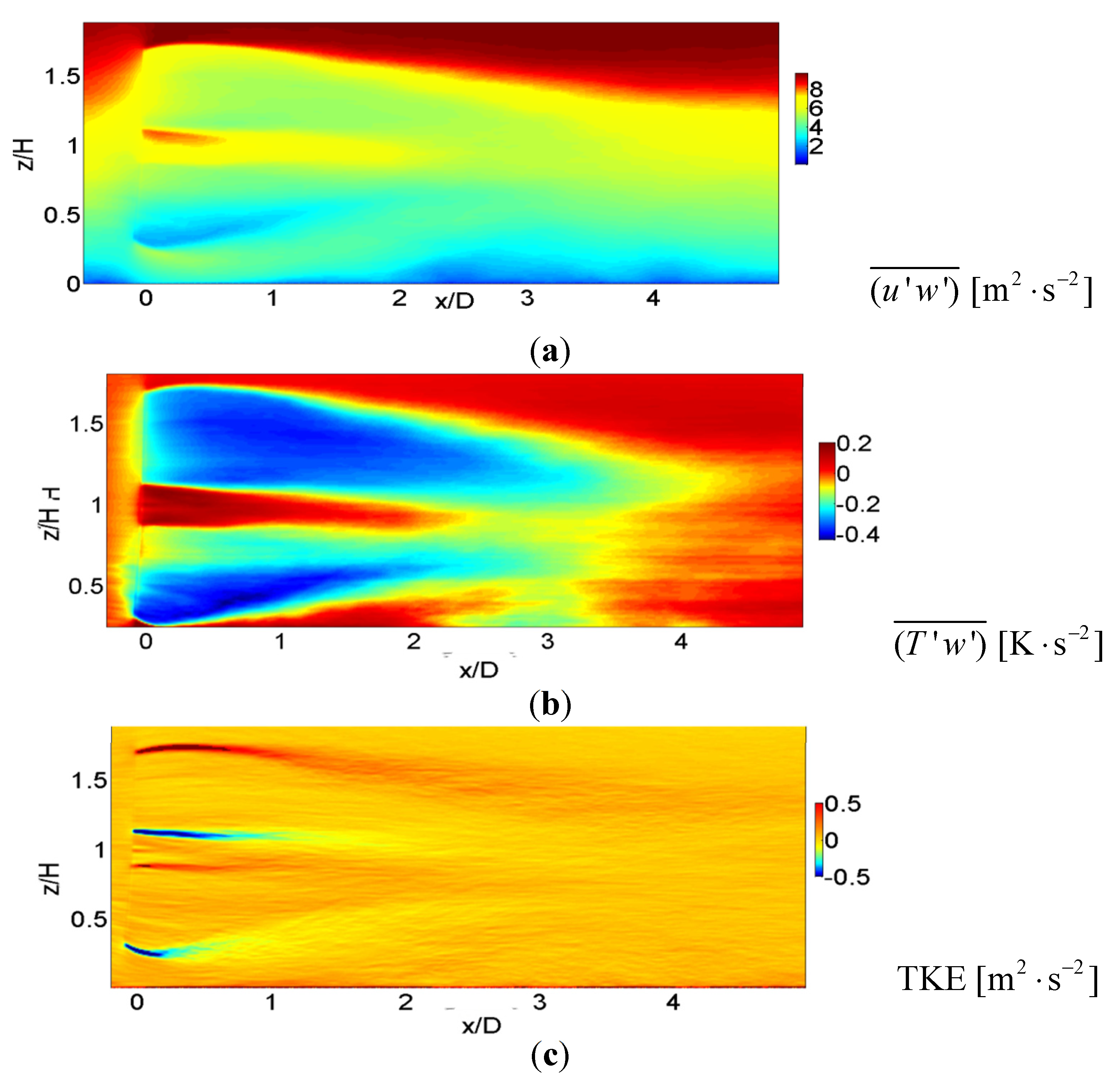
Figure 5.
Contours of time-averaged (a) Reynolds shear stress (u'w'); (b) T'w'; (c) TKE at the center plane, y/D = 0 of WT in low-stable ABL regime.
Figure 5.
Contours of time-averaged (a) Reynolds shear stress (u'w'); (b) T'w'; (c) TKE at the center plane, y/D = 0 of WT in low-stable ABL regime.
Figure 5a illustrates the contour plot of time-averaged Reynolds shear stress (
u'w') at the center plane. At the inlet of the WT, the wind is in the ABL state, wherein high shear stress is generated near the wall. Reynolds shear stress is generated due to the tip and root vortices. At the upper tip, higher shear stress is present downstream of
x/D = 1.
Figure 5b shows the contours plot of time-averaged. Strong buoyancy damping is present in the mixing layer.
Figure 5c shows the contour plot of time-averaged TKE at the center plane. High TKE is present up to
x/D = 1.5 due to the root vortices.
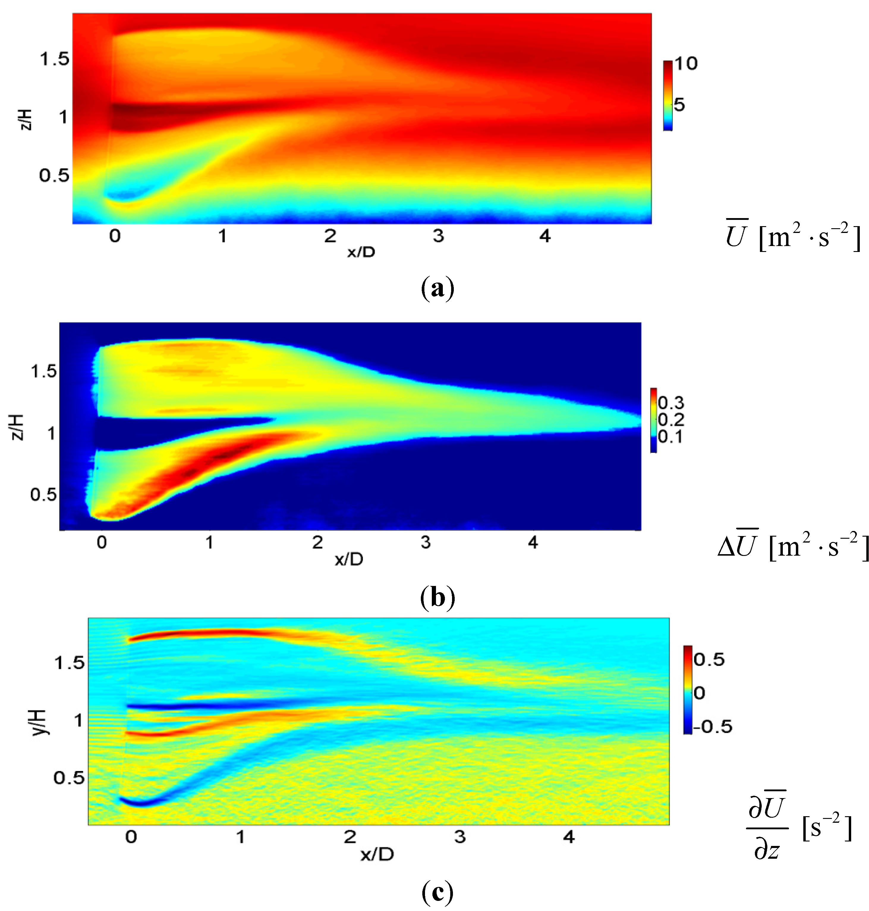
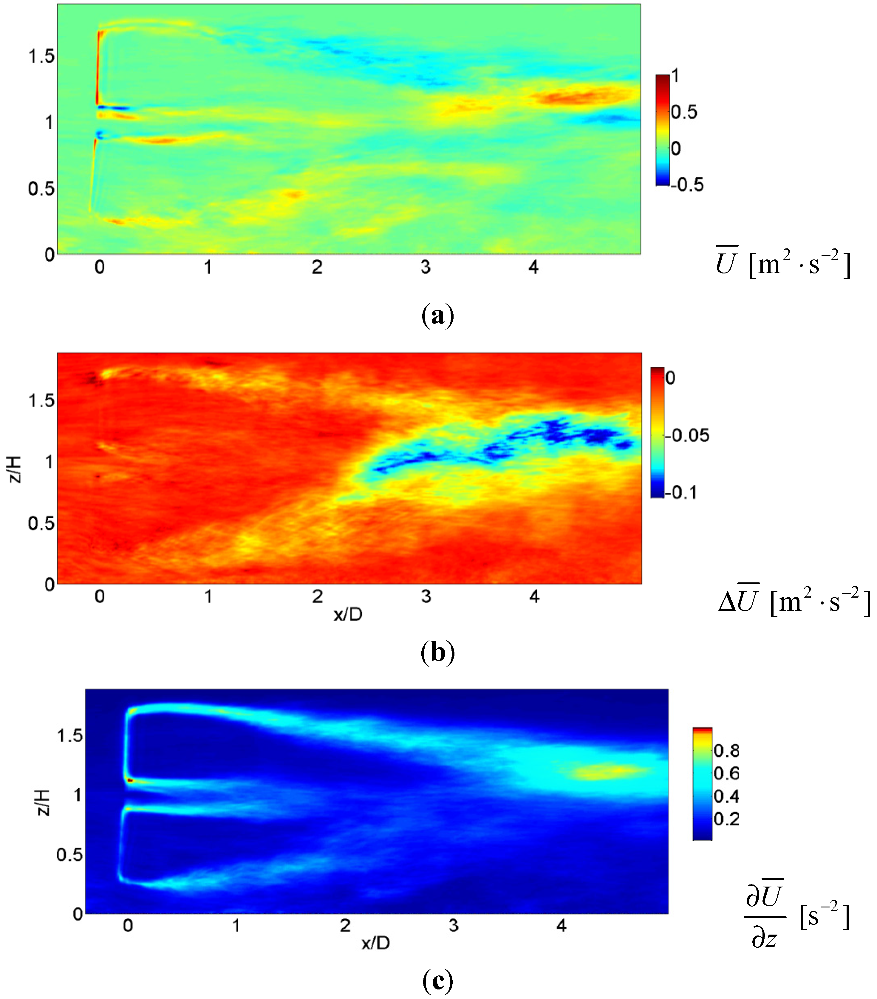
The time-averaged streamwise velocity and the velocity deficit next are presented in
Figure 6a,b, respectively. The velocity deficit is defined as follows ∆
U/
U0 = (
U −
U0)/
U0: where
U0 is the ABL velocity at the inlet of the domain. WT rotor rotation extracts the momentum from the incoming ABL flow, resulting in regions of low momentum fluid near the blade tips. Velocity deficits generated in the upper and lower regions of the wake are commensurable, resulting in a symmetric wake structure. Strong deficits of 40% of the inlet ABL velocity develop near the blade tips. The wake recovers with 10% deficit by
x/D = 4. The wake recovery is fast due to high turbulence, which is consistent with the observations of Troldborg
et al. [
37,
38]. The flow in the wake region begins to mix due to the presence of ABL turbulence.
Figure 6.
Contours of (a) time-averaged streamwise velocity; (b) deficit of time-averaged streamwise velocity; (c) mean wind shear at center plane, y/D = 0 in low-stable ABL regime.
Figure 6.
Contours of (a) time-averaged streamwise velocity; (b) deficit of time-averaged streamwise velocity; (c) mean wind shear at center plane, y/D = 0 in low-stable ABL regime.
4.2. Wake Structure of a Wind Turbine in a Moderately Stable ABL Regime
A similar analysis now is performed for the WT in the moderate-stability ABL regime.
Figure 7.
Velocity structure of the (a) Streamwise velocity; (b) Spanwise velocity; (c) wall-normal velocity, at the center plane, y/D = 0 for WT in moderately-stable ABL regime.
Figure 7.
Velocity structure of the (a) Streamwise velocity; (b) Spanwise velocity; (c) wall-normal velocity, at the center plane, y/D = 0 for WT in moderately-stable ABL regime.
The velocity structures are presented in
Figure 7. As evident from the
u velocity structures in
Figure 7a, a strong shear layer at the lower tip advects the tip vortex vertically from
z/H = −0.2 to the hub-height, where it strikes the root vortex at
x/D = 2.0. High velocity jets occur near the hub-height, which mixes with the low momentum fluid near the lower tip. Mixing is confined to the narrow hub region between the upper (from upper blade tip) and lower (from lower blade tip) shear layers. Interestingly, formed mixing layer shrinks for the moderate stability regime and it is confined to the narrow hub region (e.g., see
Figure 4). Hence, indicating the size of the mixing layer decreases with increasing stability. Further, the spanwise velocity (
Figure 7b structures) shows braid-type structures (starting at
x/D = 2.0) that differ from the large-scale coherent motions present for the WT under the low-stable ABL regime. Distinct upper-tip vortices are present up to
x/D = 2. At the same location where the lower-tip vortex strikes the root vortex, the distinct upper-tip vortices undergo a change in the stability, as demonstrated by the appearance of coherent motions. Strong shearing motion near the lower-tip is evident in
v and
w structures as well. Pockets of entraining fluid entering the WT domain from above is evident from
x/D = 2. The entraining fluid creates large-scale regions of negative velocity extending to the hub height.
Time-averaged streamwise velocity and their deficits are presented in
Figure 8a,b, respectively. Upstream of the WT, strong jets are present close to the hub-height. Due to WT rotor rotation, there is a loss of momentum at the blade tips. An asymmetric wake is created due to higher velocity deficits of 40% of the inflow velocity in the lower half of the wake (below the hub height), as well as reduced wake deficits of around 20% in the upper half of the wake. Mixing high velocity jets with low momentum fluid creates a mixing layer, and velocity deficits create a strong shear layer at the blade tips, as seen in
Figure 8c. The mixing is confined to a narrow region around the hub-height, which shrinks the shear layer downstream of the WT. The mixed layer persists up to 7D with 10% deficits, beyond which deficits decay slowly (domain not shown). It is interesting to note that upstream of the WT, the wind shear is present up to edge of the ABL (
z/H = 1.2), and above this height, the wind shear is negligible. At the same time shear now is generated at both blade tips.
Figure 8.
Time-averaged contours of (a) streamwise velocity; (b) streamwise velocity deficit; (c) wind shear (dU/dz), in the x-z plane for WT in moderate-stable ABL regime.
Figure 8.
Time-averaged contours of (a) streamwise velocity; (b) streamwise velocity deficit; (c) wind shear (dU/dz), in the x-z plane for WT in moderate-stable ABL regime.
Time-averaged Reynolds shear stress and TKE are presented in
Figure 9a,b, respectively. Reynolds stress generated at the blade tips extracts the momentum from the mean flow, creating turbulence. Additional Reynolds shear stress also is generated due to the root vortex. Further downstream, the Reynolds stress intensifies. TKE production is
![]()
; the high Reynolds shear stress region and high shear result in TKE production. However, turbulence damping occurs due to negative buoyancy production
![]()
.
Figure 9.
Time-averaged contours of (a) Reynolds shear stress; (b) TKE; (c) T'w' in the x-z plane for WT in moderate -stable ABL regime.
Figure 9.
Time-averaged contours of (a) Reynolds shear stress; (b) TKE; (c) T'w' in the x-z plane for WT in moderate -stable ABL regime.
Figure 9b shows that buoyancy flux is strong only in the lower region of the wake. The resultant TKE in the domain is a balance of the shear production and buoyant damping. Generated by the tip and root vortex, high Reynolds shear stresses create high TKE, as seen in
Figure 9c. Similar to the low-stable ABL regime, a sudden increase in the Reynolds shear stresses and TKE occurs at
x/D = 3.0. To understand the cause of this behavior, it is necessary to consider the structure of the tip vortex in detail.
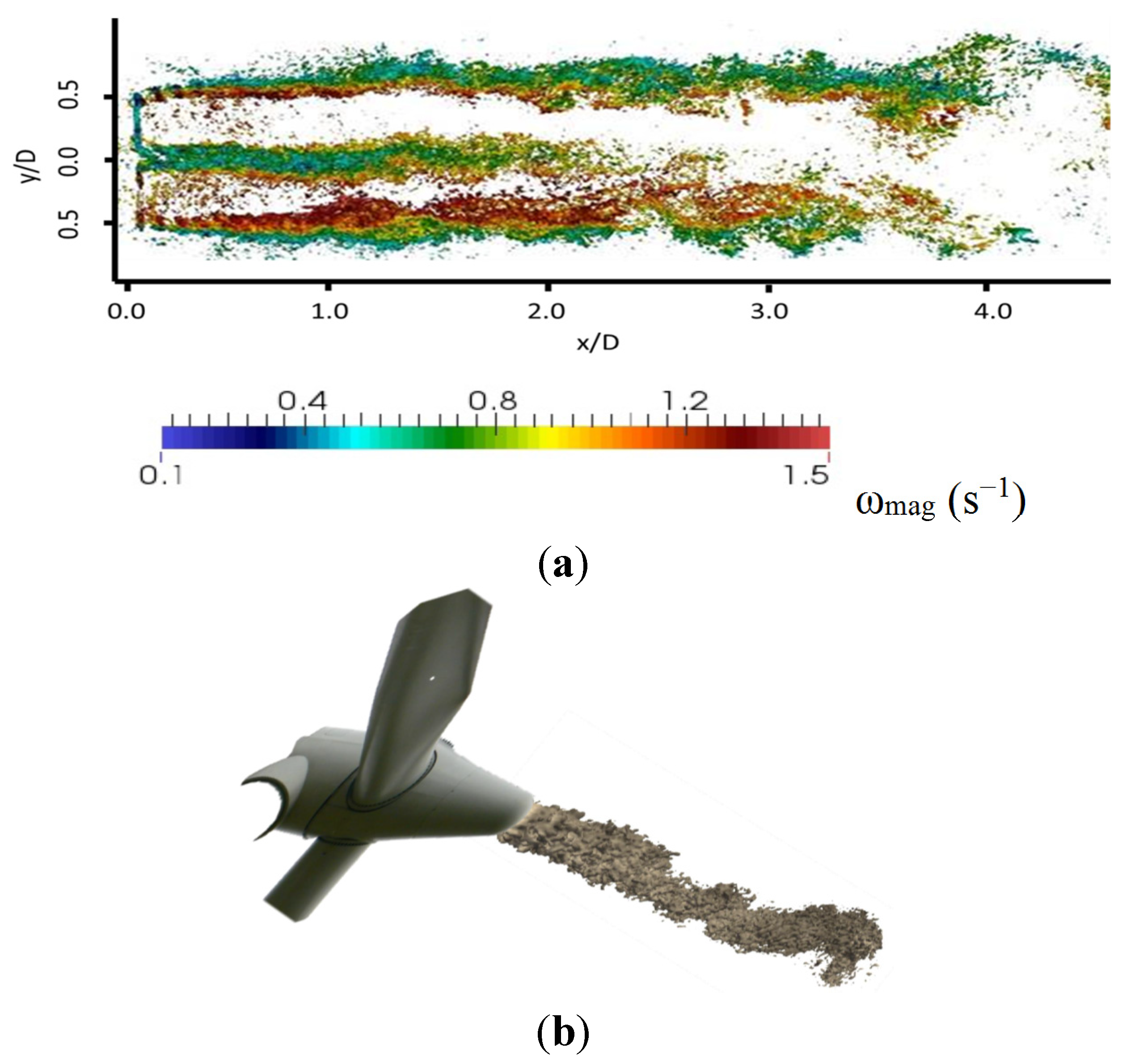
4.3. 3-D Structure of the Near-Wake Expansion: Role of ABL Wind Angle
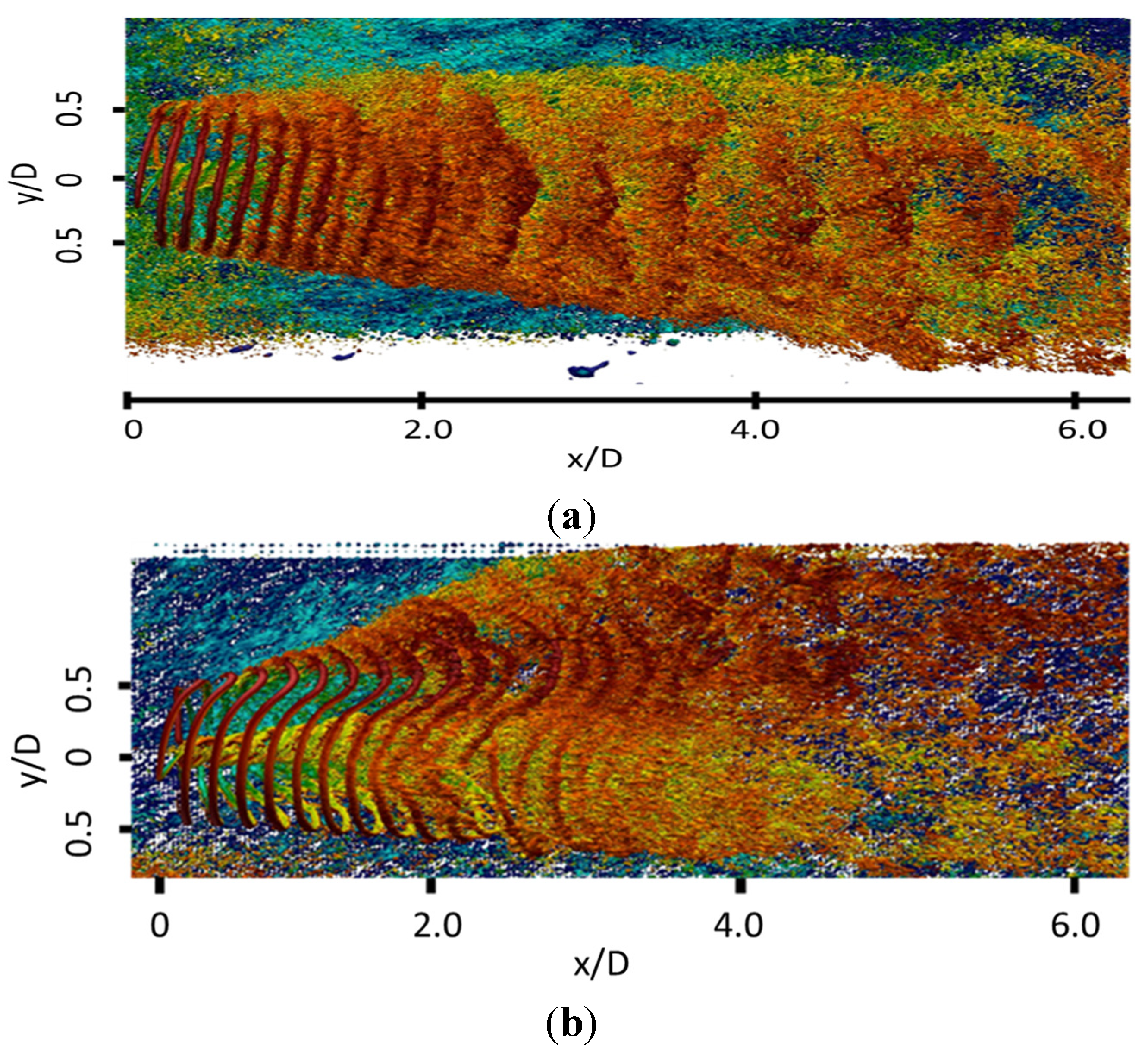
Figure 10 presents the top-view of the 3-D wake structures extracted using the λ
2 vortex detection criterion of Jeong and Hussain [
39]. The three WT blades create tip and counter-rotating root vortices, one for each blade. The tip vortex filament follows a helical trajectory. The wake structure at different ABL regimes is influenced by the height-varying wind angle, ABL inlet turbulence levels, and wind shear. The system of helical tip vortex filaments is one of the key features of WT wake structure. The tip vortices are generated due to the continuous release of vorticity at the blade tips. In the low-stable ABL regime, uniform shear and ABL turbulence act on both blade tips. The moderate stability ABL regime has non-uniform vertical shear and lower turbulence levels, which results in significant stretching of the vortex filaments, as shown in
Figure 10b. At that height, the lateral wake expansion depends on the wind angle.
Figure 10.
Structure of the wake in the horizontal plane (top-view) from the λ2 criterion (low positive values) for (a) low-stable; (b) moderate -stable ABL regimes.
Figure 10.
Structure of the wake in the horizontal plane (top-view) from the λ2 criterion (low positive values) for (a) low-stable; (b) moderate -stable ABL regimes.
Figure 11 illustrates the wake expansion with the wake at heights corresponding to
z = 30 m, 60 m, 90 m (hub-height), 120 m and 150 m. Also shown in the figure is the wind angle at that height. The WT has been placed such that it faces the wind from the west at the hub-height (θ = 270°). The corresponding wake angles have been computed with respect to the WT axis. For the low-stable ABL regime, the wind angles varies from θ = 261.75° to θ = 282.8° between the blade tips with respect to the WT axis, and the wake angle varies in a comparable manner from φ = 263° at lower tip to φ = 280.5° at upper tip of the WT blade. For the moderate-stable ABL regime, the wind angle varies from θ = 237.5°–270° with respect to the WT axis; the wake angle varies in a way comparable to φ = 238.2°–270°, thus suggesting that the approaching wind angle dictates lateral expansion at that height. Assuming a constant wind angle significantly underestimates the lateral wake expansion. Some insightful conclusions can be drawn from this figure. For the low-stable regime, the mixing layer develops downstream of the WT, and large-scale coherent structures form in the mixing layer.
Figure 11.
Velocity in the horizontal plane at heights corresponding to (a,b) z = 30 m; (c,d) z = 60 m; (e,f) 90 m; (g,h) 120 m; and (i,j) z = 150 m. (Left): low-stratified ABL and (Right): moderately-stratified ABL regimes. Shown are the wind angle and the resultant wake angle with respect to the WT.
At each of these heights, significant velocity variations exist in the transverse direction within the mixing layer. Meanwhile, velocity variations along the transverse direction are insignificant above the hub-height for the moderate stability regime.
4.4. Tip Vortex: Vortex Merging and Mutual Inductance
To further clarify the nature of the tip-vortex interactions, we present the vorticity at the upper tip for both regimes. Due to mutual induction, the spirals approach each other, resulting in a merging of the vortices with the presence of characteristic wake meandering. As two vortex filaments undergo mutual inductance, the merging process occurs, which results in both tip vortices being off-set from the idealized helical path. Numerically, the existence of vortex merging due to mutual induction was first revealed by Sorensen [
40]. Recently, Sherry
et al. [
15] studied the wake dynamics of WT in idealized uniform flow (without ABL) and demonstrated that the merging process drives the mutual inductance mode suggested by Widnall [
17].
Figure 12a,b (side view) clearly shows the upper-tip vortex, the roll up, and subsequent vortex-pairing for low-stable and moderately stable cases, respectively.
Figure 11a shows that distinct tip vortices are present close to the WT. At
x/D = 1.8, downstream of the WT, they come close together and merge. Downstream of the merge, instabilities increase, enhancing the instability of the tip vortex. For the moderate stability regime, as seen in
Figure 11b, similar vortex merging is evident around
x/D = 2.0. Downstream of the merge, strong vertical movement of the tip vortex is evident. Vortex merging generates high TKE at
x/D = 3.0 (
Figure 9) and results in entraining the flow from above (
Figure 7c).
Figure 13 shows the top view of the vorticity contours of the upper-tip vortex. The spacing between vortex number
n = 1–7 is fixed and depends on the tip-speed ratio. Mutual induction occurs between vortex number 8 & 9 and 10 & 11 as the spacing between them decreases, eventually resulting in vortex merging (see
Figure 13a). For the low stable regime, the background ABL is strong, and strong shearing motion acts on the helical spiral. For the moderately stable regime, a similar vortex merging process occurs for vortex number
n = 8 & 9, resulting in the vortex merging between
n = 10 & 11 and 12 & 13.
Figure 12.
Spanwise slice of isocontours of the vorticity field of the upper tip-vortex has been isolated for WT in (a) low-stable; (b) moderately-stable ABL regime. The distinct upper-tip vortices merge to form vortex blobs and they evolve downstream. The contour levels correspond to (0.5–2.0 1/s).
Figure 13.
Top view of iso-contours of the vortex field that has been isolated near the tip vortex for the WT in (a) low-stable; (b) moderate -stable ABL regime. Iso-contour levels corresponding to (0.5–2.0 1/s) have been presented.
Figure 13.
Top view of iso-contours of the vortex field that has been isolated near the tip vortex for the WT in (a) low-stable; (b) moderate -stable ABL regime. Iso-contour levels corresponding to (0.5–2.0 1/s) have been presented.
4.5. Wake Meandering: Role of ABL Turbulence and Wind Shear
Downstream of the WT, significant spanwise variation of the velocity (from
Section 4.2) and the existence of vortex merging due to mutual inductance (from
Section 4.3) clearly suggest the possibility of lateral meandering of the wake. For this purpose, we isolate the region from
z/D = 0.8–1.1 and
y/D = ±0.5 from the central plan (statistics have revealed spanwise variations are insignificant beyond this transverse distance from the central plane). The velocity contours are shown in
Figure 14a. Further, from
Figure 14a, we isolate the hub region to reveal the meandering of the root vortex in
Figure 14b. The velocity contours clearly indicate meandering of the wake. Interestingly, the root vortex begins swirling and meandering motions occur from
x/D = 0.9. The hub vortex deviates by
y/D = ±0.5 from the central plane (
y/D = 0) (measured as the distance at which spanwise gradients are less than 1% of peak gradients). Kang, Wang and Sotiropoulos [
19] observed similar wake meandering behavior and attributed it to the onset of the spiral mode of vortex breakdown at the hub region.
In the mixing layer that develops behind the WT, the tip vortex filaments undergo roll up, leading to large-scale coherent structures. The distinct tip vortices undergo vortex merging and roll up around x/D = 0.9, causing Reynolds shear stress to increase. Further increases in Reynolds stresses arises when the shear layer from the lower-tip vortex strikes the root vortex between x/D = 2–3 (depending on y/D location), suggesting enhanced meandering motions. For the moderate stability regime, the large-scale instabilities that develop from the roll-up of the tip-vortices are different. Enhanced Reynolds shear stress due to striking of the lower-tip vortex on the root vortex is evident; however, no significant meandering has been observed (figure not shown).
Figure 14.
Wake meandering of the root vortex in low-stable regime: (a) magnitude of vorticity at the hub-height; (b) iso-contours of velocity in the region x/D = 0–3.5, z/H = 0.8–1.1, y/D= −0.5 to 0.5 velocity contours in the range of (2–5 m/s) have been isolated.
Figure 14.
Wake meandering of the root vortex in low-stable regime: (a) magnitude of vorticity at the hub-height; (b) iso-contours of velocity in the region x/D = 0–3.5, z/H = 0.8–1.1, y/D= −0.5 to 0.5 velocity contours in the range of (2–5 m/s) have been isolated.
5. Conclusions
We have conducted an LES-based numerical study in order to understand the near-wake structure of full-scale WTs subjected to stably stratified ABL under low- and moderate stability regimes. The study is one of the first to account for real time atmospheric conditions, including atmospheric mean state, turbulence, wall stresses, and heat flux. In a stable ABL, the structure of the atmosphere is complicated by the existence of LLJs in the mean flow, height-varying wind angle, wind shear, and turbulence levels. ABL conditions significantly govern lateral wake expansion. The resultant turbulence in the ABL is a balance of the shear-generated turbulence and buoyancy damping. Increasing stability influences the wind characteristics by altering both the shear production and buoyancy dissipation of turbulence. The study has isolated the wind characteristics relevant to turbine wake structure, ABL metrics including height-varying wind shear, wind angle and turbulence, and LLJs.
WT blade rotation causes a momentum deficit at the blade tips, resulting in low momentum fluid near the tips. Shear layers are developed at the lower- (lower shear layer) and upper-blade (upper shear layer) tips due to the root vortex. In the low-stable ABL regime, uniform wind shear and buoyancy damping create a symmetric wake. High ABL turbulence develops a mixing layer downstream of the WT. The wake recovery is fast due to high turbulence. In the moderate stability ABL regime, asymmetric wake is created due to non-uniform ABL wind shear. A mixing layer forms between the upper- and lower-shear layers in a narrow region around the hub-height. High TKE due to upper shear layer persists up to 7D downstream, whereas TKE is damped at the lower shear layer because of buoyancy damping. Hence, wake decay is slow with an asymmetric wake persisting further downstream in the far wake region. In the wake region, additional source of Reynolds shear stress production occurs as a result of the following: (i) vortex merging, (ii) striking of tip and root vortices due to ABL mean shear. The resultant TKE generated from the augmented Reynolds shear stress depends on the mean wind shear at that height.
Lateral wake expansion is significant for stable ABL flows. For the low-stable ABL regime, the wind angles vary from θ = 261.75°–282.8°; with respect to the WT axis between z = 30 m–150 m, the wake angle varies in a comparable manner from φ = 263°–280.5°. For the moderate-stable ABL regime, the wind angle varies from θ = 237.5°–270° with respect to the WT axis; the wake angle varies in a way comparable to φ= 238.2°–270°, thus suggesting that the approaching wind angle dictates the lateral expansion at that height.
For WT under stable ABL conditions, tip and root vortices that are generated due to blade vorticity undergo two distinct regimes: (i) tip vortices are essentially unstable in stratified ABL and undergo mutual induction, resulting in vortex merging. Vortex merging augments the exiting Reynolds shear stress; and (ii) the stratified mixing layer that forms downstream of the vortex merging undergoes an instability, forming large-scale coherent structures. The low-stable and moderately stable ABL regimes differ in that the low-stable regime Reynolds stress generated due to vortex merging enhances the TKE production due to uniform wind shear (note that TKE production =
![]()
). However, the tip vortex is outside the ABL for moderately-stable regime; hence, the vortex merging process does not generate additional TKE. Further, as the strength of the mixing length reduces with increasing stability, the well-defined coherent structures of the mixing layer formed in the low-stable ABL regime disappear in the moderate stability regime. Instead, braided and connected forms of structures become evident. This study is one of the first to confirm vortex merging due to mutual inductance form of instability and the instability of the mixing layer together play an important role in wake meandering.
The study is offered as an important contribution to our understanding of ABL-driven WT wakes in a stably-stratified atmosphere. The stratified turbulent mixing layer formed downstream of the WT is influenced by ABL metrics, thus dictating the wake dynamics, including lateral wake expansion, tip/root vortex instabilities, instability of the mixing layer, and wake recovery. Future studies in wake effects of WT should account for realistic atmospheric turbulence and wind angle in addition to wind shear and mean forcing conditions. In atmospheric flows, the pressure gradient is a balance of the Coriolis forcing and Reynolds shear stress; hence, idealistic studies with specified pressure gradients grossly underestimate the lateral wake expansion. We strongly recommend that future studies account for realistic pressure gradients obtained from momentum balance equations.

 denotes the modified pressure. The spatial gradient of the mean pressure term acts to drive the flow convection, (u1, u2, u3) = (u, v, w) are the components of the velocity field (u is the axial component; v is the lateral or y-component; and w is the vertical component).
  is the resolved potential temperature; θ0 is the reference temperature. The subgrid stresses (SGS) are included in the τ term along with the fluid stress tensor. The SGS flux and SFS temperature flux are parameterized, respectively as follows:
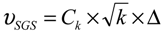 and
and 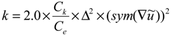 , Δ = (ΔxΔyΔz)1/3 using the mesh cells in x, y and z directions, the resolved strain-rate tensor is, and PrSGS is constant (ref dependent on stratification level).
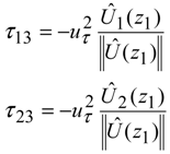


 ; the high Reynolds shear stress region and high shear result in TKE production. However, turbulence damping occurs due to negative buoyancy production
  .
.


 ). However, the tip vortex is outside the ABL for moderately-stable regime; hence, the vortex merging process does not generate additional TKE. Further, as the strength of the mixing length reduces with increasing stability, the well-defined coherent structures of the mixing layer formed in the low-stable ABL regime disappear in the moderate stability regime. Instead, braided and connected forms of structures become evident. This study is one of the first to confirm vortex merging due to mutual inductance form of instability and the instability of the mixing layer together play an important role in wake meandering.