A Model-Free Approach for Maximizing Power Production of Wind Farm Using Multi-Resolution Simultaneous Perturbation Stochastic Approximation

Abstract
:
1. Introduction
2. Problem Formulation
3. Multi-Resolution Simultaneous Perturbation Stochastic Approximation
3.1. Standard Simultaneous Perturbation Stochastic Approximation
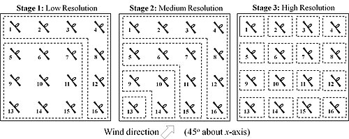
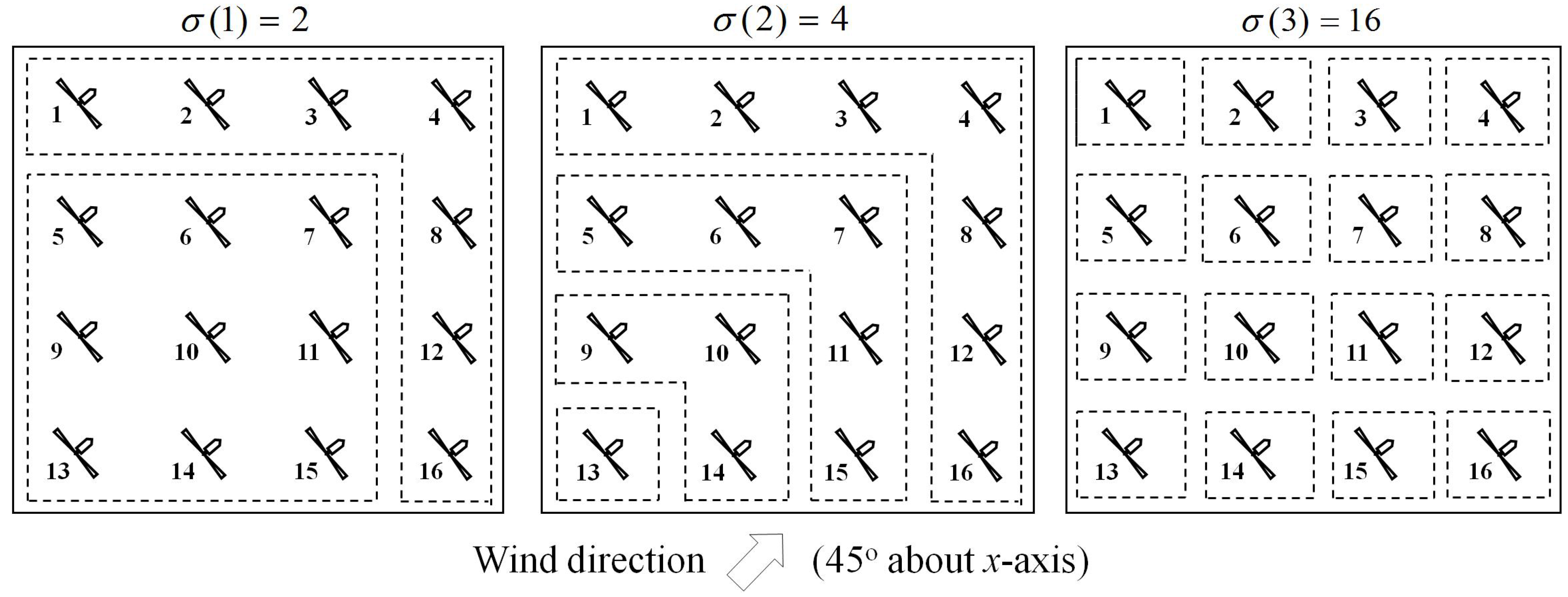
3.2. Multi-Resolution Simultaneous Perturbation Stochastic Approximation
- (i)
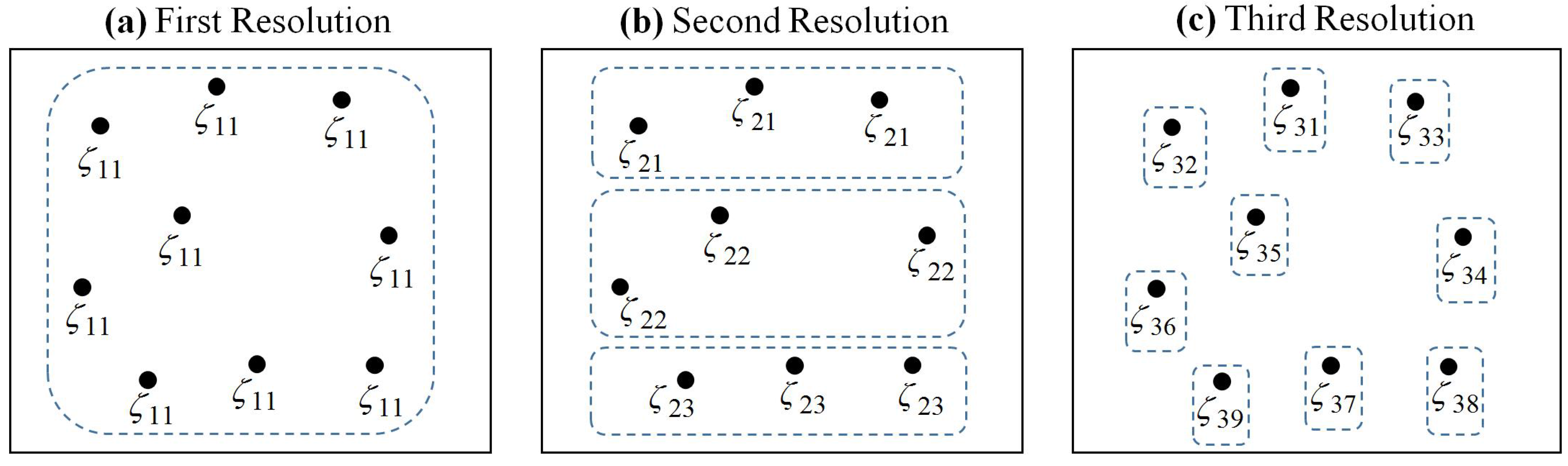
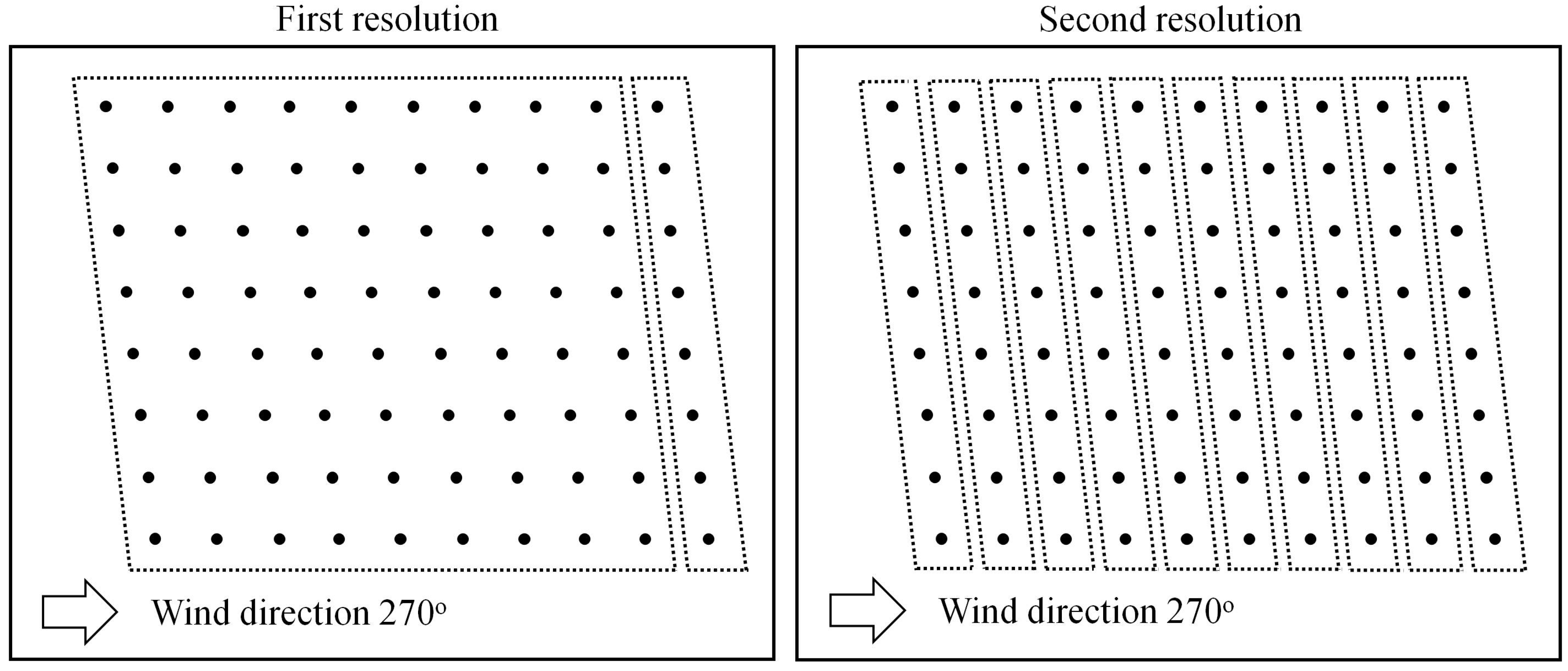
- First Resolution (j = 1):for h(1)(ζ1) = [ζ11 ζ11 · · · ζ11]T ∈ ℝ9, where ζ1 = ζ11 ∈ ℝ is shown in Figure 1a and ζ1(0) ∈ ℝ is the given initial condition. Note that the design parameters, which are grouped in the box with a dashed line, have the same value.
- (ii)
- Second Resolution (j = 2):for h(2)(ζ2) = [ζ21 ζ21 ζ21 ζ22 ζ22 ζ22 ζ23 ζ23 ζ23]T ∈ ℝ9, where ζ2 = [ζ21 ζ22 ζ23]T ∈ ℝ3 is shown in Figure 1b and ζ2(0) = []T.
- (iii)
- Third Resolution (j = 3):for h(3)(ζ3) = [ζ31 ζ32· · · ζ39]T ∈ ℝ9, where ζ3 = [ζ31 ζ32· · · ζ39]T ∈ ℝ9 is shown in Figure 1c and ζ3(0) = []T. After obtaining , the optimal solution is given by θ∗ := .
4. Model-Free Design for Maximizing Total Power Production of Wind Farm

5. Simulation Results
5.1. Wind Farm Model
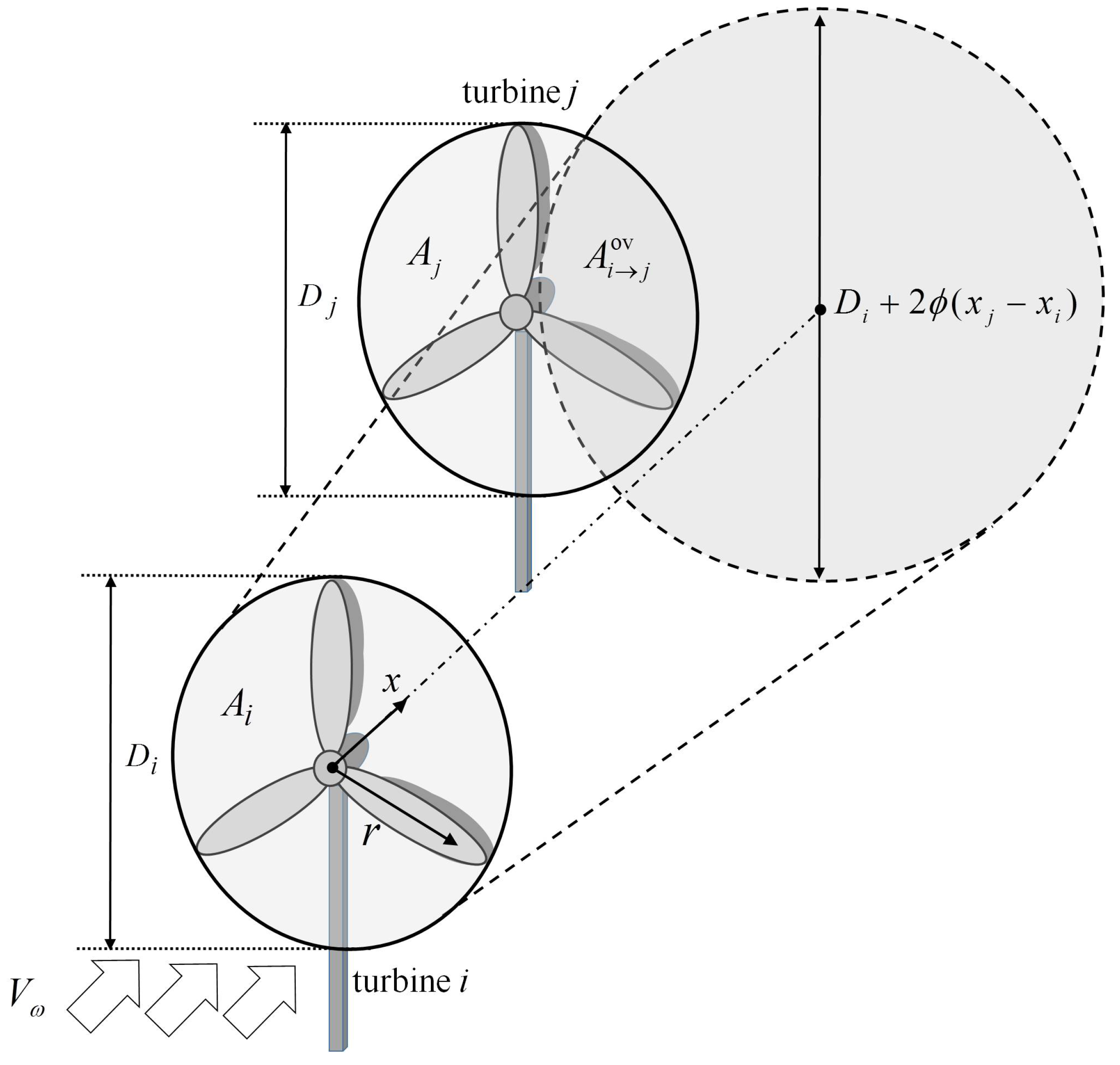
 = {1, 2, ..., p} be the set of p wind turbines in the wind farm, Vω be the incoming wind speed, Di be the rotor diameter of the turbine i, Aj be the rotor swept area of turbine j, be the overlap area between the wake generated by an upstream turbine i and rotor swept area of turbine j, and ø is a roughness coefficient that represents the slope of wake expansion. Let also (x, r) be a point in the wake of the turbine, where x is the distance to the rotor disk plane of the turbine and r is the distance to the centerline of the wind turbine rotor axis. Then, the aggregate wind velocity is given by:
 is evaluated based on the aggregation of the wind velocity deficit created by each upstream turbine. We also assume that the diameter of the wake has a circular cross-section and expands proportionally to the distance x. Further, the power of each turbine can be represented as:


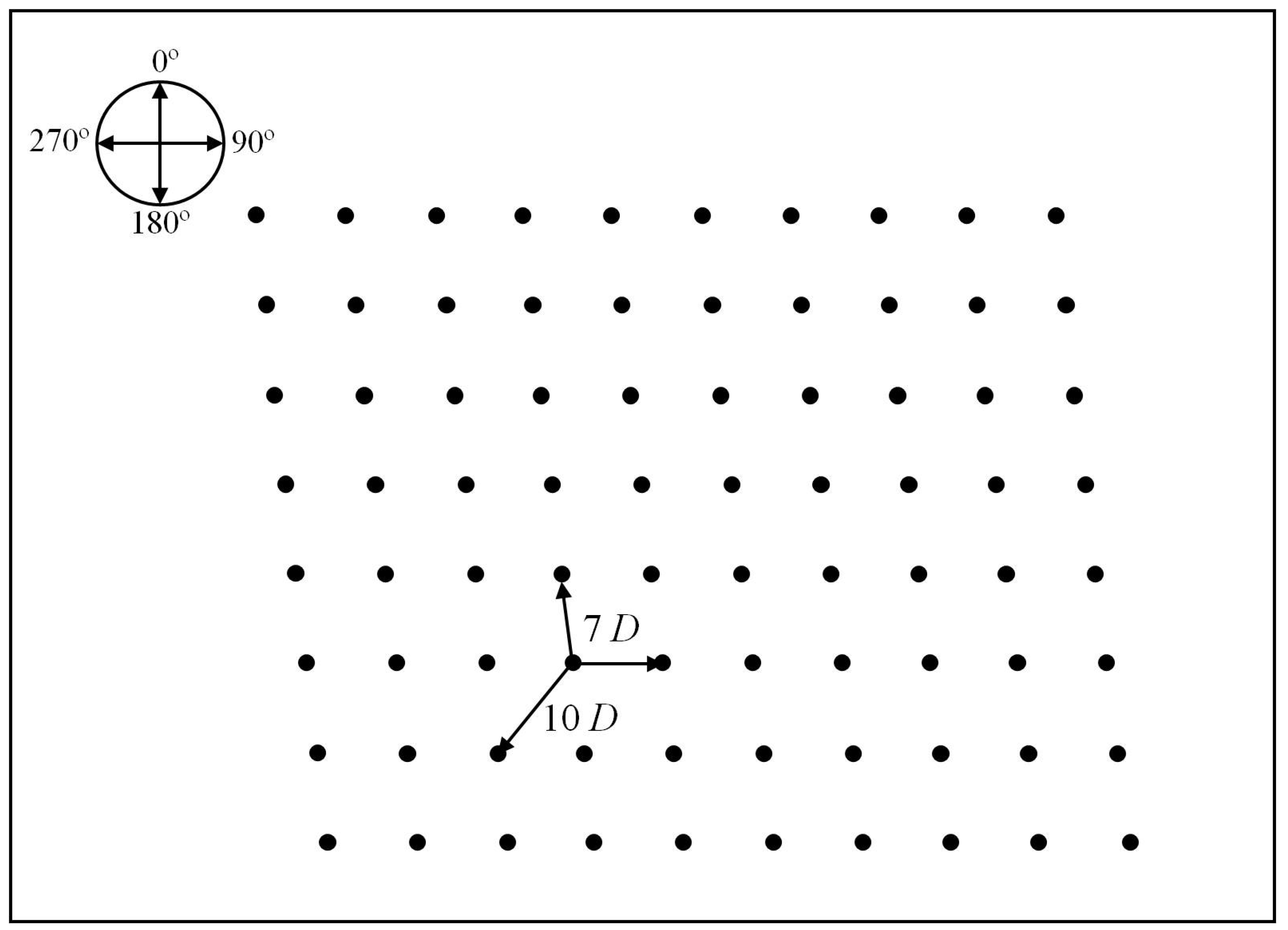
5.2. Horns Rev Example
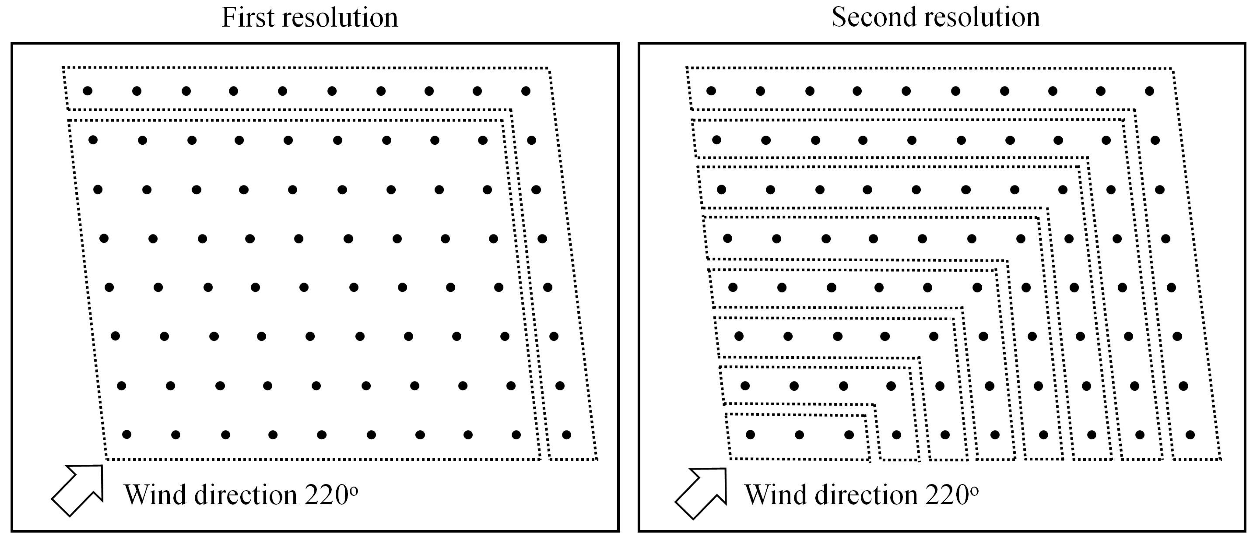
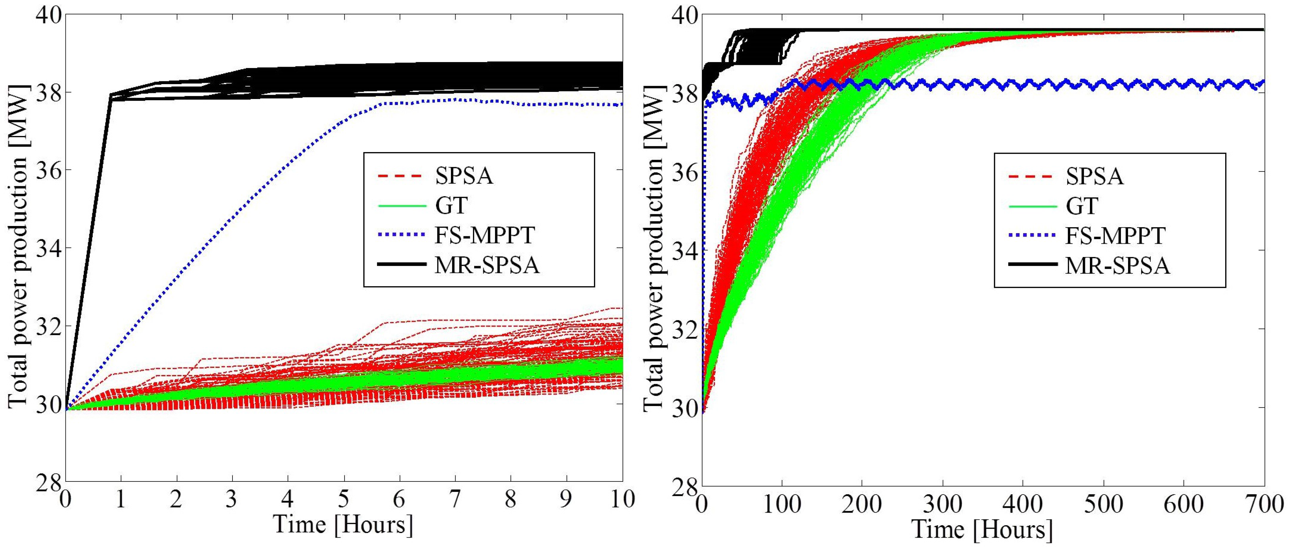
5.2.1. Performance of the MR-SPSA-Based Algorithm with Different Wind Directions


| Wind Direction | SPSA | GT | FS-MPPT | MR-SPSA | |
|---|---|---|---|---|---|
| 170° | Mean | 39.5909 | 39.5814 | - | 39.6056 |
| Best | 39.6010 | 39.5897 | 38.3153 | 39.6056 | |
| Worst | 39.5701 | 39.5678 | - | 39.6056 | |
| Std. (×10–3) | 6.1145 | 3.7439 | - | 0.0042 | |
| 200° | Mean | 57.8567 | 57.8436 | - | 57.8582 |
| Best | 57.8576 | 57.8494 | 57.7861 | 57.8582 | |
| Worst | 57.8546 | 57.8393 | - | 57.8582 | |
| Std. (×10–3) | 0.6113 | 2.1246 | - | 0.0071 | |
| 220° | Mean | 48.2179 | 48.2022 | - | 48.2246 |
| Best | 48.2236 | 48.2129 | 47.7155 | 48.2260 | |
| Worst | 48.2083 | 48.1914 | - | 48.2194 | |
| Std. (×10–3) | 3.8714 | 3.9699 | - | 1.1286 | |
| 240° | Mean | 57.1734 | 57.1622 | - | 57.1788 |
| Best | 57.1769 | 57.1679 | 57.0917 | 57.1788 | |
| Worst | 57.1668 | 57.1544 | - | 57.1786 | |
| Std. (×10–3) | 1.9807 | 2.3574 | - | 0.0346 | |
| 250° | Mean | 63.6910 | 63.6780 | - | 63.6931 |
| Best | 63.6923 | 63.6837 | 63.6818 | 63.6931 | |
| Worst | 63.6889 | 63.6704 | - | 63.6931 | |
| Std. (×10–3) | 0.7166 | 2.6241 | - | 0.0064 | |
| 270° | Mean | 38.0758 | 38.0867 | - | 38.1187 |
| Best | 38.1038 | 38.0986 | 37.0026 | 38.1187 | |
| Worst | 37.9935 | 38.0733 | - | 38.1182 | |
| Std. (×10–3) | 20.5476 | 5.5781 | - | 0.0517 |
| Wind Direction | SPSA | GT | FS-MPPT | MR-SPSA | |
|---|---|---|---|---|---|
| 170° | Mean | 178.9725 | 225.4735 | - | 11.7518 |
| Best | 124.1333 | 185.3833 | 5.3333 | 4.9000 | |
| Worst | 227.8500 | 265.9611 | - | 29.4000 | |
| Std. | 19.8712 | 13.7529 | - | 5.5497 | |
| 200° | Mean | 145.5825 | 107.6600 | - | 3.2025 |
| Best | 113.2500 | 87.0000 | 5.6669 | 2.2500 | |
| Worst | 200.2500 | 127.2500 | - | 6.7500 | |
| Std. | 18.8706 | 7.9725 | - | 1.0437 | |
| 220° | Mean | 236.8800 | 227.2239 | - | 7.5950 |
| Best | 180.8333 | 185.5000 | 5.5600 | 4.6667 | |
| Worst | 318.5000 | 266.0000 | - | 19.8333 | |
| Std. | 27.3979 | 14.2829 | - | 3.0688 | |
| 240° | Mean | 195.2800 | 147.8800 | - | 4.3800 |
| Best | 141.0000 | 124.3333 | 5.7500 | 3.0000 | |
| Worst | 263.0000 | 177.0000 | - | 12.0000 | |
| Std. | 22.0097 | 10.8787 | - | 2.0090 | |
| 250° | Mean | 199.3845 | 122.1185 | - | 4.0740 |
| Best | 145.9500 | 85.7500 | 5.6000 | 3.1500 | |
| Worst | 240.4500 | 155.0500 | - | 10.5000 | |
| Std. | 22.1671 | 14.6361 | - | 1.4101 | |
| 270° | Mean | 228.8895 | 293.1180 | - | 6.3000 |
| Best | 152.2500 | 261.1000 | 4.9400 | 2.1000 | |
| Worst | 318.1500 | 350.7000 | - | 18.9000 | |
| Std. | 28.6038 | 17.3374 | - | 4.0101 |
| Performance | H1 | H2 | H3 | H4 | |
|---|---|---|---|---|---|
| Total power production (MW) | Mean | 48.2240 | 48.2249 | 48.2244 | 48.2247 |
| Best | 48.2260 | 48.2262 | 48.2261 | 48.2266 | |
| Worst | 48.2168 | 48.2224 | 48.2209 | 48.2195 | |
| Std. (×10−3) | 1.4639 | 0.8374 | 0.9187 | 0.9688 | |
| Convergence time (h) | Mean | 7.3383 | 7.7467 | 8.2017 | 7.4200 |
| Best | 4.6667 | 4.6667 | 4.6667 | 4.6667 | |
| Worst | 15.1667 | 17.5000 | 16.3333 | 17.5000 | |
| Std. | 2.8253 | 2.9872 | 3.2045 | 2.8020 |
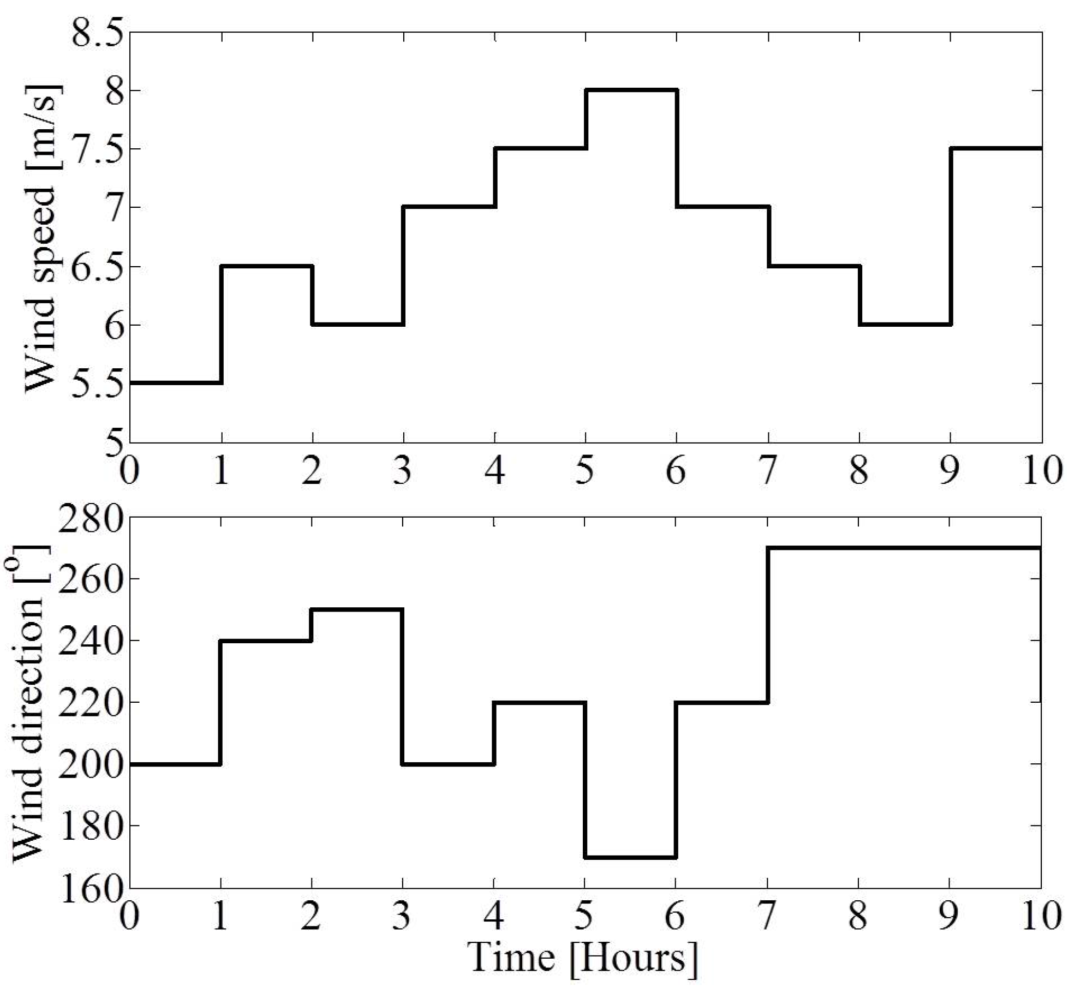
5.2.2. Performance of the MR-SPSA-based Algorithm with Non-Static Incoming Wind

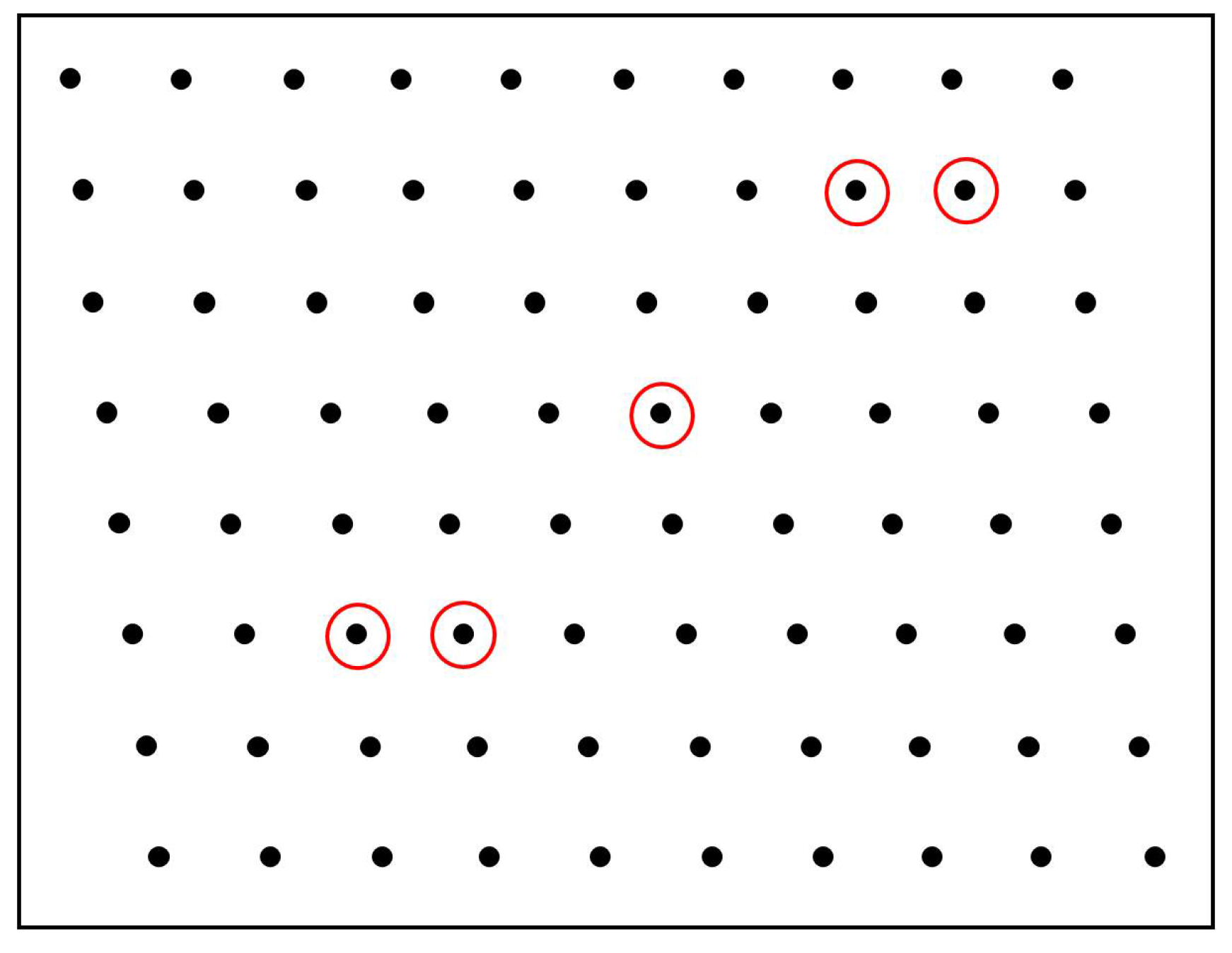
5.2.3. Performance of the MR-SPSA-based Algorithm with Turbine Failures

| Performance | SPSA | GT | FS-MPPT | MR-SPSA | |
|---|---|---|---|---|---|
| Total power production (MW) | Mean | 36.3817 | 36.3902 | - | 36.4134 |
| Best | 36.4065 | 36.3971 | 35.6525 | 36.4141 | |
| Worst | 36.3381 | 36.3791 | - | 36.4113 | |
| Std. (×10−3) | 13.0305 | 4.1416 | - | 0.5158 | |
| Convergence time (h) | Mean | 216.5100 | 272.4295 | - | 3.0555 |
| Best | 155.4000 | 245.0000 | 5.0167 | 2.1000 | |
| Worst | 285.6000 | 307.6500 | - | 8.4000 | |
| Std. | 28.2459 | 14.8820 | - | 1.7346 |
6. Conclusions
Acknowledgments
Author Contributions
Notation
| p | Number of wind turbines in the wind farm |
| ai | Control parameter of turbine i |
| a | Control parameter vector of the turbines in the wind farm |
| Pi | Power production of turbine i |
Total power production of the wind farm | |
| n | Number of design parameters |
| f | Objective function for ℝn → ℝ |
| θ, θ∗ | Design parameter vector |
| ã, c, Ã, α, γ | Nonnegative coefficients of SPSA parameter |
| △(k) | Random perturbation vector at k-th step |
| △i(k) | i-th component of △(k) |
| ε | Small number |
| q | Resolution step |
| σ(j) (j = 1, 2, ..., q) | Number of design parameters at each resolution j |
| h(j)(j = 1, 2, ..., q) | Function for ℝσ(j)→ℝn at each resolution j |
| ζj, (j = 1, 2, ..., q) | Design parameter vector at each resolution j |
| ζjk (j = 1, 2, ..., q) | k-th component of ζj |
| Gjk (k = 1, 2, ..., σ(j)) | Groups of the wind turbine at each resolution j |
| nk | Number of turbines in the group |
| | Set of p wind turbines in the wind farm |
| Vω | Incoming wind speed |
| Di | Rotor diameter of the turbine i |
| Aj | Rotor swept area of turbine j |
Overlap area between the wake generated by an upstream turbine i and Aj | |
| ø | Roughness coefficient |
| x | Distance to the rotor disk plane of the turbine |
| r | Distance to the centerline of the wind turbine rotor axis |
Aggregate wind velocity | |
| ρ | Air density |
| m(i) (i = 1, 2, ..., p) | Index of the nearest neighbor downstream turbine of turbine i |
| (i) (i = 1, 2, ..., p) | Set of turbine i and other downstream turbines in a row that are affected by turbine i |
| Tw | Time interval for the wake to travel to the whole wind farm |
| KF | Scaling factor for the size of the design parameter step in the FS-MPPT-based method |
| KG | Size of interval for random step on the design parameter in the GT-based method |
| E | Probability of using a new random setting in the GT-based method |
Conflicts of Interest
References
- Laks, J.H.; Pao, L.Y.; Wright, A.D. Control of wind turbines: Past, present, and future. In Proceedings of the American Control Conference, St. Louis, MO, USA, 10–12 June 2009; pp. 2096–2103.
- Pao, L.Y.; Johnson, K. Control of wind turbines. IEEE Control Syst. Mag. 2011, 31, 44–62. [Google Scholar]
- Johnson, K.; van Wingerden, J.W.; Balas, M.J.; Molenaar, D.-P. Special issue on “Past, present and future modeling and control of wind turbines”. Mechatronics 2011, 21. [Google Scholar] [CrossRef]
- Hansen, A.; Sorensen, P.; Iov, F.; Blaabjerg, F. Centralised power control of wind farm with doubly fed induction generators. Renew. Energy 2006, 31, 935–951. [Google Scholar]
- Spudic, V.; Baotic, M.; Jelavic, M.; Peric, N. Hierarchical wind farm control for power/load optimization. In Proceedings of the Conference Science of Making Torque from Wind, Crete, Greece, 28–30 June 2010; pp. 681–692.
- Spudic, V.; Jelavic, M.; Baotic, M. Wind Turbine Power Control for Coordinated Control of Wind Farms. In Proceedings of the 18th International Conference on Process Control, Tatranska Lomnica, Slovakia, 14–17 June 2011; pp. 463–468.
- Soleimanzadeh, M.; Wisniewski, R. Controller design for a wind farm, considering both power and load aspects. Mechatronics 2011, 21, 720–727. [Google Scholar]
- Soleimanzadeh, M.; Wisniewski, R.; Kanev, S. An optimization framework for load and power distribution in wind farms. J. Wind Eng. Ind. Aerodyn. 2012, 107–108, 256–262. [Google Scholar]
- Madjidian, D.; Rantzer, A. A stationary turbine interaction model for control of wind farms. In Proceedings of the 18th IFAC World Congress, Milano, Italy, 28 August 2011; pp. 4921–4926.
- Bitar, E.; Seiler, P. Coordinated control of a wind turbine array for power maximization. In Proceedings of the American Control Conference, Washington, DC, USA, 17–19 June 2013; pp. 2898–2904.
- Marden, J.R.; Ruben, S.D.; Pao, L.Y. Surveying game theoretic approaches for wind farm optimization. In Proceedings of the AIAA Aerospace Sciences Meeting, Nashville, TN, USA, 6–9 January 2012; pp. 1–10.
- Marden, J.R.; Ruben, S.D.; Pao, L.Y. A model-free approach to wind farm control using game theoretic methods. IEEE Trans. Control Syst. Technol. 2013, 21, 1207–1214. [Google Scholar]
- Park, J.; Kwon, S.; Law, K.H. Wind farm power maximization based on a cooperative static game approach. In Proceedings of the SPIE 8688, Active and Passive Smart Structures and Integrated Systems, San Diego, CA, USA, 10 March 2013.
- Gebraad, P.M.O.; van Dam, F.C.; van Wingerden, J.-W. A model-free distributed approach for wind plant control. In Proceedings of the American Control Conference, Washington, DC, USA, 17–19 June 2013; pp. 628–633.
- Ahmad, M.A.; Azuma, S.I.; Baba, I.; Sugie, T. Switching controller design for hybrid electric vehicles. SICE J. Control Meas. Syst. Integr. 2014. Accepted for publication. [Google Scholar]
- Bianchi, F.; Battista, H.D.; Mantz, R. Wind Turbine Control Systems; Principles, Modelling and Gain Scheduling Design; Springer-Verlag: London, UK, 2007. [Google Scholar]
- Spall, J.C. Multivariate stochastic approximation using a simultaneous perturbation gradient approximation. IEEE Trans. Autom. Control 1992, 37, 332–341. [Google Scholar]
- Spall, J.C.; Hill, S.D.; Stark, D.R. Theoretical comparisons of evolutionary computation and other optimization approaches. In Proceedings of the Congress on Evolutionary Computation, Washington, DC, USA, 6–9 July 1999; pp. 1398–1405.
- Scholbrock, A. Optimizing wind farm control strategies to minimize wake loss effects. Master’s Thesis, University of Colorado Boulder, Boulder, CO, USA, July 2011. [Google Scholar]
- Sorensen, T.; Thogersen, M.L.; Nielsen, P.; Grotzner, A.; Chun, S. Adapting and Calibration of Existing Wake Models to Meet the Conditions Inside Offshore Wind Farms; EMD International A/S: Aalborg, Denmark, 2008. [Google Scholar]
- Katic, I.; Højstrup, J.; Jensen, N.O. A simple model for cluster efficiency. In Proceedings of the European Wind Energy Conference, Rome, Italy, 7–9 October 1986; pp. 407–410.
- Porté-Agel, F.; Wu, Y.T.; Chen, C.H. A numerical study of the effects of wind direction on turbine wakes and power losses in a lar ge wind farm. Energies 2013, 6, 5297–5313. [Google Scholar]
© 2014 by the authors; licensee MDPI, Basel, Switzerland. This article is an open access article distributed under the terms and conditions of the Creative Commons Attribution license (http://creativecommons.org/licenses/by/4.0/).
Share and Cite
Ahmad, M.A.; Azuma, S.-i.; Sugie, T. A Model-Free Approach for Maximizing Power Production of Wind Farm Using Multi-Resolution Simultaneous Perturbation Stochastic Approximation. Energies 2014, 7, 5624-5646. https://doi.org/10.3390/en7095624
Ahmad MA, Azuma S-i, Sugie T. A Model-Free Approach for Maximizing Power Production of Wind Farm Using Multi-Resolution Simultaneous Perturbation Stochastic Approximation. Energies. 2014; 7(9):5624-5646. https://doi.org/10.3390/en7095624
Chicago/Turabian StyleAhmad, Mohd Ashraf, Shun-ichi Azuma, and Toshiharu Sugie. 2014. "A Model-Free Approach for Maximizing Power Production of Wind Farm Using Multi-Resolution Simultaneous Perturbation Stochastic Approximation" Energies 7, no. 9: 5624-5646. https://doi.org/10.3390/en7095624
APA StyleAhmad, M. A., Azuma, S.-i., & Sugie, T. (2014). A Model-Free Approach for Maximizing Power Production of Wind Farm Using Multi-Resolution Simultaneous Perturbation Stochastic Approximation. Energies, 7(9), 5624-5646. https://doi.org/10.3390/en7095624