Article

An Acceleration Slip Regulation Strategy for Four-Wheel Drive Electric Vehicles Based on Sliding Mode Control

National Engineering Laboratory for Electric Vehicles, Beijing Institute of Technology, Beijing 100081, China
*
Author to whom correspondence should be addressed.
Energies 2014, 7(6), 3748-3763; https://doi.org/10.3390/en7063748
Submission received: 28 January 2014 / Revised: 15 May 2014 / Accepted: 3 June 2014 / Published: 17 June 2014
(This article belongs to the Special Issue Advances in Hybrid Vehicles)

Abstract

:
This paper presents an acceleration slip regulation (ASR) system for four-wheel drive (4WD) electric vehicles, which are driven by the front and rear axles simultaneously. The ASR control strategy includes three control modes: average distribution of inter-axle torque, optimal distribution of inter-axle torque and independent control of optimal slip rate, respectively, which are designed based on the torque adaptive principle of inter-axle differential and sliding mode control theory. Furthermore, in order to accurately describe the longitudinal tyre force characteristic, a slip rate calculation formula in the form of a state equation was used for solving the numerical problem posed by the traditional way. A simulation was carried out with the MATLAB/Simulink software. The simulation results show that the proposed ASR system can fully use the road friction condition, inhibit the drive-wheels from slipping, and improve the vehicle longitudinal driving stability.

1. Introduction

Although the dynamic performance of four-wheel drive (4WD) conventional vehicles is improved compared with that of two-wheel drive vehicles, the fuel economy is relatively poor. It’s worth noting that a purely electric vehicle can completely ignore the impact of fuel economy [1,2]. Considering the motor has the characteristics of low speed and high torque, a pure electric vehicle that employs the 4WD scheme can not only improve the vehicle’s acceleration and climbing performance, but also have a positive impact for reducing emissions and air pollution [3,4,5]. However, the chassis layout of a high power motor is usually difficult due to its large volume, but a good distribution layout scheme can divide one high power and large volume size motor into several small motors, thus realizing a flexible chassis layout and improving the vehicle’s dynamic performance reliability [6,7,8,9].
Electric vehicles have several advantages such as a drive wheel torque that can be acquired easily, sensitive motor response, and motor torque that can be controlled accurately, etc. Therefore, the advantages of acceleration slip regulation (ASR) application in an electric vehicle are incomparable to those seen in a conventional vehicle. Not only PID (Proportion Integration Differentiation) control, but also several techniques based on nonlinear control have been applied to ASR research [10,11]. A fuzzy logic control was introduced in ASR control in [12]. Nakakuki et al. [13] proposed the linearization feedback control for the ASR function. Sliding mode control enables the system architecture having the switching characteristics changes over time, forces the system into doing the small amplitude and high frequency movement along a predetermined state trajectory with a certain characteristic, and the control theory was studied by many scholars due to its good robustness [14,15,16,17,18]. The key technology of ASR is how to balance the relationship between the driver demand torque, the tyre characteristics and the road friction conditions [19]. This paper undertakes a specific analysis of these three elements, and an ASR strategy which contains three control modes is designed for good roads, slippery roads and bad roads, and the motor output torque is controlled based on sliding control theory. The simulation results show that the proposed ASR system can choose the suitable control mode according to the different road friction conditions and take full advantage of the road friction, thus improves the vehicle’s longitudinal driving stability.

2. System Model

In this paper, the 4WD electric vehicle ASR system layout was as shown in Figure 1. The power battery pack provides power to the two identical power and volume motors, and the ASR controller sends the control command in the form of torque control to the two motors, thus the two motors simultaneously output power externally by directly connecting to the differentials of the front and rear axles.
Figure 1. The four-wheel drive (4WD) electric vehicle acceleration slip regulation (ASR) system layout.
Energies 07 03748 g001

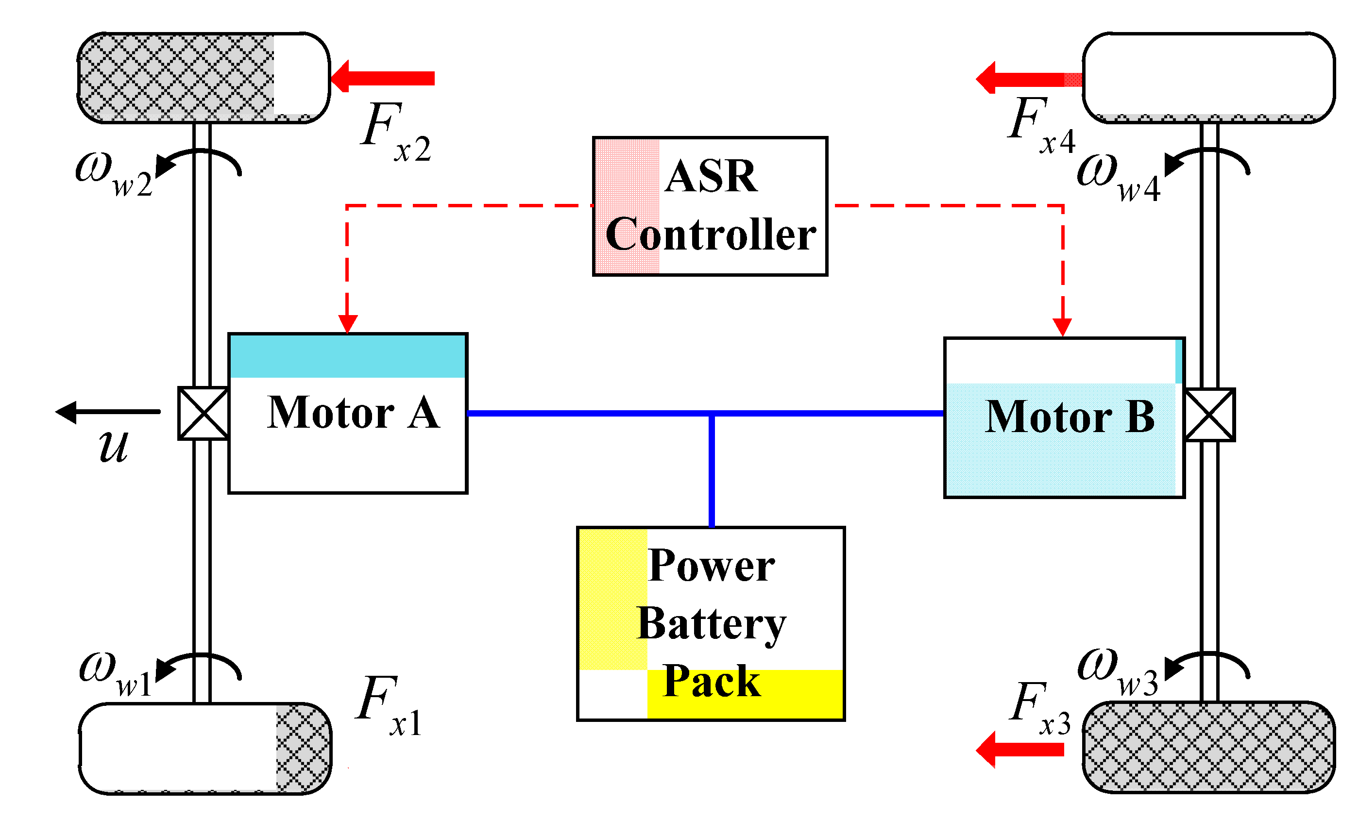
2.1. Vehicle Dynamics Model

Since this paper focuses on the influence of ASR on the vehicle’s longitudinal dynamic performance, the vehicle dynamics model adopted here contains five degrees of freedom as seen in Figure 1, the five degrees of freedom include the vehicle longitudinal motion and the rotational movement of the four wheels. According to the Newton’s law, the motion equations of the vehicle are derived as follows [20]:
(1) Vehicle longitudinal movement:
Energies 07 03748 i001
where u is longitudinal velocity of vehicle, m is vehicle mass, Fxi is tyre longitudinal force.
(2) Four wheel’s rotation movement:
Energies 07 03748 i002
where ωwi is wheel angular velocity, Iwi is wheel rotation inertia, rw is rolling radius of the tyre, Tmi is motor driving torque.

2.2. Tyre Model

The tyre dynamics are usually modeled with the “Magic Formula” developed by Pacejka et al. [21] which employs combinations of trigonometric functions to describe the tyre forces exactly. In this model, the tyre longitudinal force is described as the complex nonlinear function of the slip rate and tyre vertical load. Thus, the tyre longitudinal force model can be expressed as the following equation:
Fxi = D sin{C arctan[BXE(BX − arctan BX)]}
where B, C, D, E are the stiffness, shape, peak, curvature factor, respectively. X is the input vector for this model. All of them are described as the function of the tyre vertical load Fz, tyre slip rate λ and relevant fitting coefficient bi, the fitting coefficients are shown in Table 1 and the specific description can be shown as follows:
Energies 07 03748 i003
Table 1. “Magic Formula” fitting coefficients.
No.012345
bi1.0231621.80968526.23360.09624250.331460.00906
No.678910
bi−0.002550.037260.87693−0.00009−0.00033

2.3. Motor Model

In this paper, permanent magnet synchronous motors were chosen for constructing the dual-motor drive system. The motor’s rated torque is 270 Nm and the rated power is 90 kW. Motor models are usually mainly divided into the theoretical model and the quasi- steady-state model. This paper adopted the latter one and plotted the motor external characteristic curve according to the characteristic motor parameters, and acquired the motor speed and peak torque according to the load signal namely the accelerator open degree, then adopted one-order inertia to complete the dynamic correction on the motor output torque as the following equation:
Energies 07 03748 i004
where Tm is the motor’s output torque, Tmax is the motor’s peak torque, α is the degree of openness of the accelerator, τm is the motor’s responsive time constant, n is the motor speed, nN is the inflection point speed of the motor’s external curve.

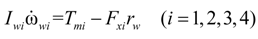
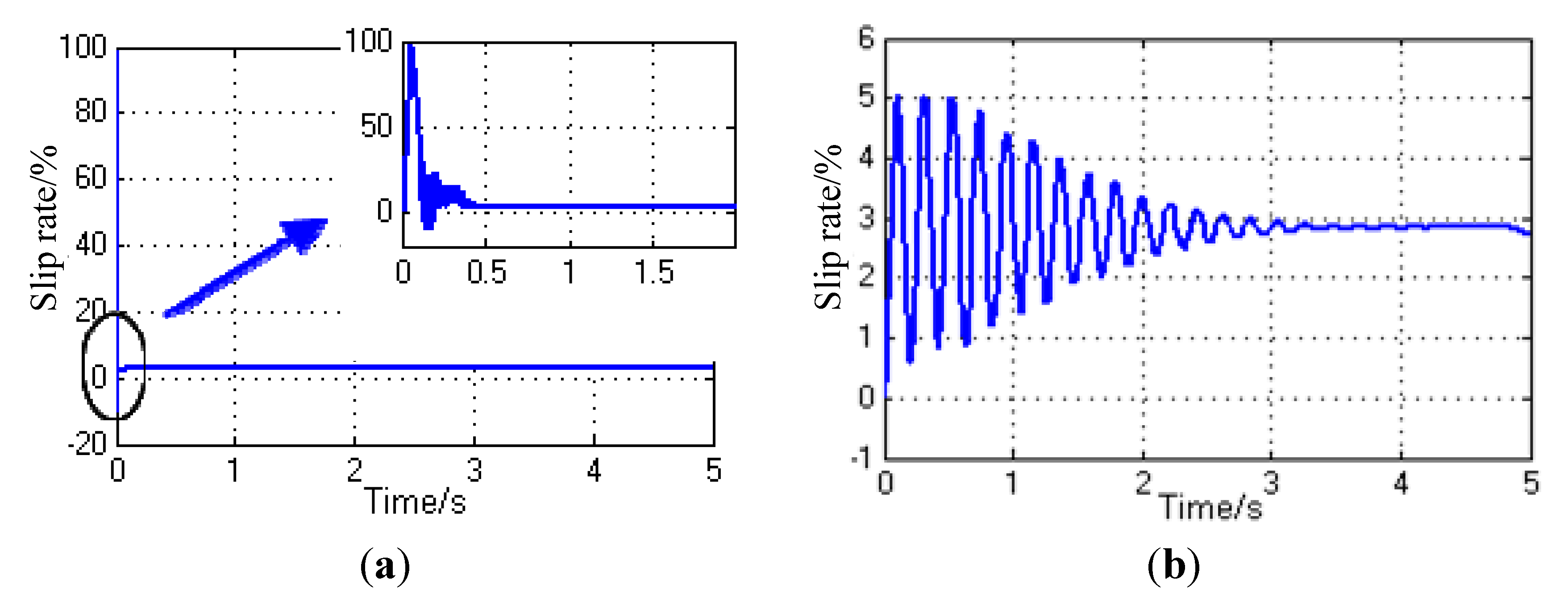
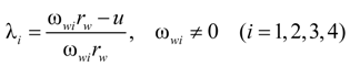
2.4. Slip Rate Calculation Model

The tyre slip rate is the key factor for tyre longitudinal force calculation, the relationship among slip rate, wheel speed and vehicle velocity can be expressed as follows:
Energies 07 03748 i005
The wheel speed ωwi and vehicle velocity u are very small when the vehicle is in transient starting, and a numerical problem such as λi → ∞ is likely to occur when using Equation (5), it is evidently inconsistent with the force characteristics of tyre contact points. To solve this problem, this paper adopts a modified slip rate calculation method which was proposed by Bernard [22]. Hence the Equation (6) can be changed into a state Equation (7) of ωwi and u:
Energies 07 03748 i006
where σx = Cs/Cx, Cs is the tyre longitudinal slip stiffness, Cx is tyre shear stiffness.
The simulation results of tyre slip rate are shown in Figure 2, which are calculated by Equations (5) and (6) respectively. Obviously, using the state equation to describe slip rate is more in line with the vehicle real starting process.
As shown in Figure 2b, the tyre slip rate fluctuates significantly in the initial stage, this is because |rrωi|/σx in the Equation (6) can be regarded as small spring damping coefficient when the vehicle velocity is low, namely the description of tyre slip rate is similar to that of a circular spring. Therefore, it is necessary to modify Equation (7) as follows [15]:
Energies 07 03748 i007
Energies 07 03748 i008
where ∆λi is the modifying factor for slip rate, λi is the modified slip rate, ulow is the low vehicle velocity threshold.
Figure 2. Comparison of two methods for tyre slip rate calculation: (a) Simulation results of Equation (6); (b) Simulation results of Equation (7).
Energies 07 03748 g002
The simulation result of the modified tyre slip rate is shown in Figure 3, where we can see that the curve fluctuation in the initial stage was effectively smoothed, proving that the Equation (8) can better describe the tyre slip rate, especially at low vehicle velocity.
Figure 3. The modified tyre slip rate at a low vehicle velocity.
Energies 07 03748 g003

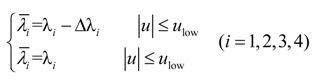
3. Control Strategies

The cause of tyre slip phenomena is that the wheel drive torque exceeds the torque which is provided by the road adhesion limitation, and its essence is the balanced relationships between maximum drive torque, road adhesion conditions and the driver-desired torque. For the 4WD electric vehicle in this paper, the maximum drive torque is the motor’s maximum torque, the road adhesion conditions are expressed by the product of the road drive force and wheel radius, namely Troad = Fx × Rw, and the driver desired torque Td was obtained from the acceleration pedal signal αpedal (0–1), namely Tdesire = αpedal × (Tf_max + Tr_max), where Tf_max and Tr_max are the maximum torque values of the front and rear motors, and both of them are equal due to their identical characteristic parameters, namely Tf_max = Tr_max = Tmax. So it can be simplified that Td = αpedal ×2 × Tmax and evidently Td ≤ 2 × Tmax. The specific analysis of the balance relationships between maximum drive torque, road adhesion conditions and driver-desired torque is given as follows:
(1)
Td ≤ 2 × TmaxTroad, generally corresponds to a condition of high road adhesion. In this case, the drive wheel slip will not happen over the entire range of the accelerator pedal, and it’s not necessary to perform a complex torque distribution for the front and rear axles, just let αf = αr = αpedal. Although the slip rates of the front and rear axles will be different with the same drive torque due to the different vertical loads of front and rear axles, the vehicle dynamic performance and driving stability will not be influenced.
(2)
TdTroad ≤ 2 × Tmax, generally corresponds to the condition of middle road adhesion. In this case, although the driver-desired torque Td is smaller than Troad, the slip phenomenon may happen on the driving shaft with a smaller axle load due to the bad road conditions. So a reasonable allocation of the drive torque of the front and rear axles is required to ensure Tf + Tr = Td, thereby avoiding slipping under the condition of avoiding vehicle dynamics loss.
(3)
2 × TmaxTdTroad, generally corresponds to the condition of low road adhesion. In this case, the driver-desired torque Td is bigger than Troad, and the inter-axle torque distribution will cause an unavoidable slip phenomenon. In order to make full use of the road adhesion, the independent control for front and rear axles is the best control plan, thus the slip rates of the front and rear axles can be controlled to be equal to the optimal rate slip. In this way Tf + Tr = Troad, and the vehicle can acquire the biggest power at this moment.
In a word, the control flow of acceleration slip regulation strategy is as shown in Figure 4.
Figure 4. The acceleration slip regulation strategy.
Energies 07 03748 g004
The specific control algorithm is mainly divided into three control modes as follows.

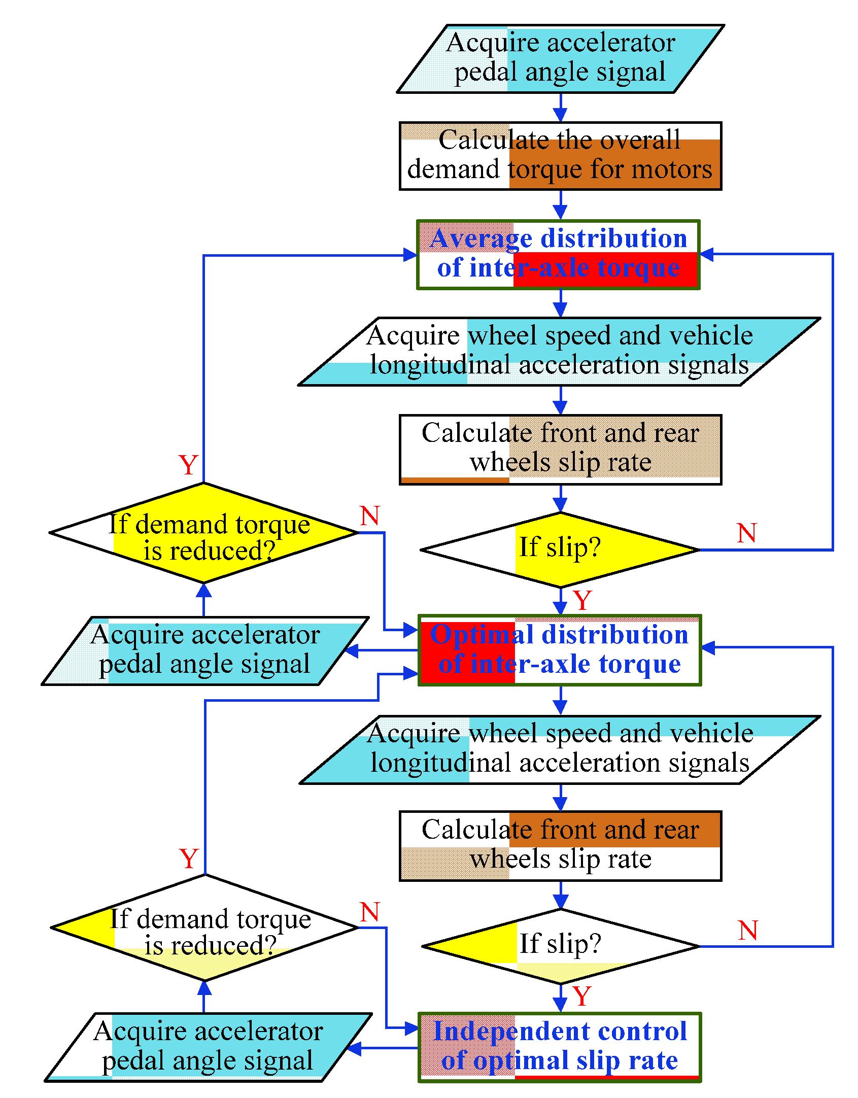
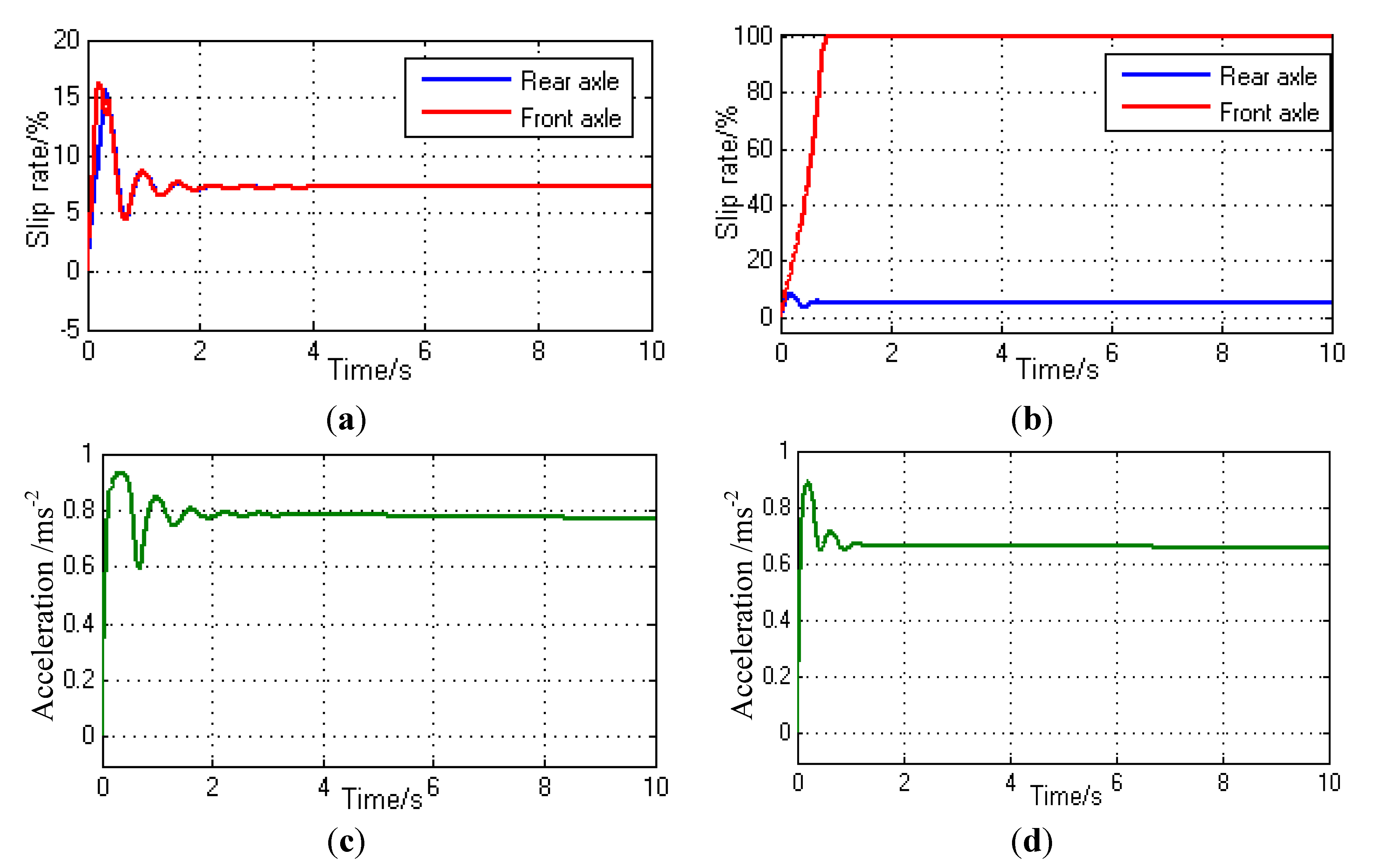
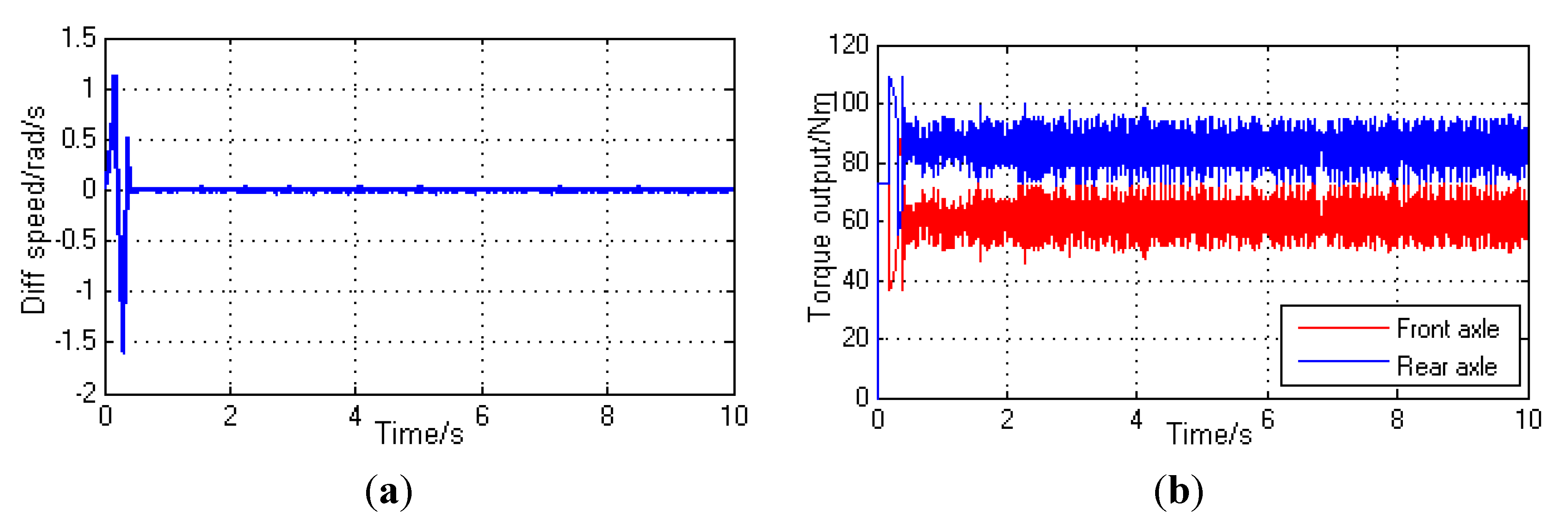
3.1. Mode 1: Average Distribution of Inter-Axle Torque

This control mode equally assigns the demand torque into the front and rear axle:
Tfa = Tra = Tdesire / 2
where Tfa and Tra are the torque of the front and rear motors with the Mode 1 control, respectively.

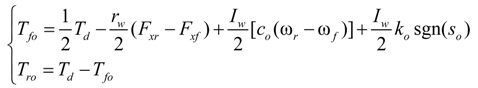
3.2. Mode 2: Optimal Distribution of Inter-Axle Torque

If the slip phenomenon occurred, this control mode will be adopted. The slip phenomenon determining condition is as follows: the front axle slip rate λf > a or the rear axle slip rate λr > a, where a is the slip threshold and its range is [0.1, 0.2]. Sliding model theory was used here to design the output torque of motors, the switching function So and reaching law o were defined in the Equations (11) and (12), respectively:
Energies 07 03748 i009
o = −ko sgn(So)
where co is the constant switching function coefficient with Mode 2 control, ko is the non-negative reaching coefficient with Mode 2 control, ωf and ωr are the front and rear axle angular velocity, respectively.
It can be found by substituting Equations (2) and (12) into Equation (11) after derivation:
Energies 07 03748 i010
where Tfo and Tro are the torque of the front and rear motors with the Mode 2 control, respectively.

3.3. Mode 3: Independent Control of Optimal Slip Rate

If the slip phenomenon still occurred after Mode 2 control was adopted, this control mode will be adopted here to control the two motors independently and ensure the slip rate of front and rear axle are equal. The switching functions sfi, sri and reaching laws fi, ri were defined in Equations (14) and (15), respectively:
Energies 07 03748 i011
Energies 07 03748 i012
where λo is the optimal slip rate and its range is [0.15, 0.2], cfi and cri are the constant switching function coefficients with Mode 3 control, kfi and kri are the reaching coefficients of non-negative with Mode 3 control.
It can be found using the same reasoning that:
Energies 07 03748 i013

4. Simulation Results and Analysis

Under the premise of ensuring the vehicle’s longitudinal stability, acceleration slip regulation is proposed to improve the vehicle’s dynamic performance. To verify the validity and accuracy of the control strategy, first, different control modes for fixed conditions were subjected to separate simulation analyses, then the effective switching between different control modes for variable condition were verified by simulation. The simulation experiments were carried out using the MATLAB/Simulink (MathWorks, Natick, MA, USA) environment, and the model parameters are as listed in Table 2.
Table 2. Simulation parameters.
ParametersValuesParametersValues
co500kri80
cfi50m5000 kg
cri500nN4000
Cs1.81 kg·m2rw0.447 m
Cx1.65 kg·m2ulow1.83 m/s
Iw2.035 kg·m2τm200
ko−100σx0.91
kfi−200

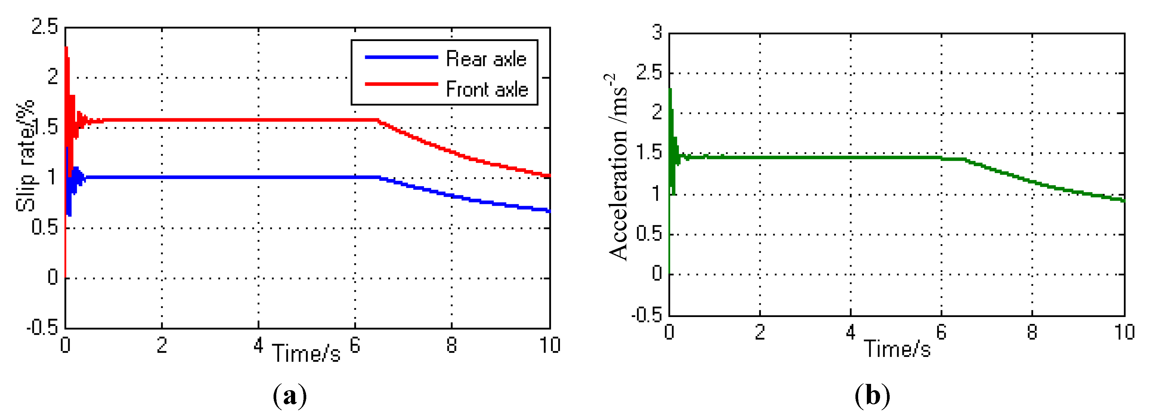
4.1. Simulation on Average Distribution of Inter-Axle Torque

When the vehicle is traveling on a high adhesion road, the average distribution of inter-axle torque model is used to control the load signal of the front and rear axle drive motor αf = αr = αpedal. The simulation results are shown in Figure 5 when the signal of the accelerator pedal αpedal = 0.5 and the peak road adhesion coefficient μH = 0.80.
As Figure 5a shows, the front and rear axle tyre slip rate varies around different stable values because of the axle loads, but they were all in a stable slip zone, Figure 5b shows that the vehicle acceleration began to stabilize at around 1.48 m/s2 under these conditions, then due to the motor speed increase, the vehicle acceleration will be reduced gradually when the motor workspace transforms from the constant torque to the constant power region.
Figure 6 shows the simulation of the distribution of the front and rear axle drive torque by axle load under these conditions. Figure 6a shows that the driver-demanded torque is distributed to the front and rear axles by the axle load so that the front and rear axle tyre slip rate can be equal. However, by comparing Figure 6b and Figure 5b, it can be known that vehicle acceleration is consistent under both torque distribution modes, and the vehicle dynamics aren’t affected.
Although the slip rate can be guaranteed to be a constant based on the torque distribution by the front and rear axle loads, in the view of the project realization, the accurate estimation of dynamic load of the front and rear axle when the vehicle is running requires a large number of external sensors, so the controller cost is expensive. In contrast, the average distribution of inter-axle torque control is simple and low cost, etc., although inconsistent tyre slip rate will lead to different front and rear tyre wear, but as long as there is enough road adhesion ability, the vehicle’s dynamic performance can’t be affected.
Figure 5. Simulation results of average distribution of inter-axle torque on good roads: (a) The front and rear axle tyre slip rate; (b) Vehicle acceleration.
Energies 07 03748 g005
Figure 6. Simulation results of torque distribution by axle load on good roads: (a) The front and rear axle tyre slip rate; (b) Vehicle acceleration.
Energies 07 03748 g006

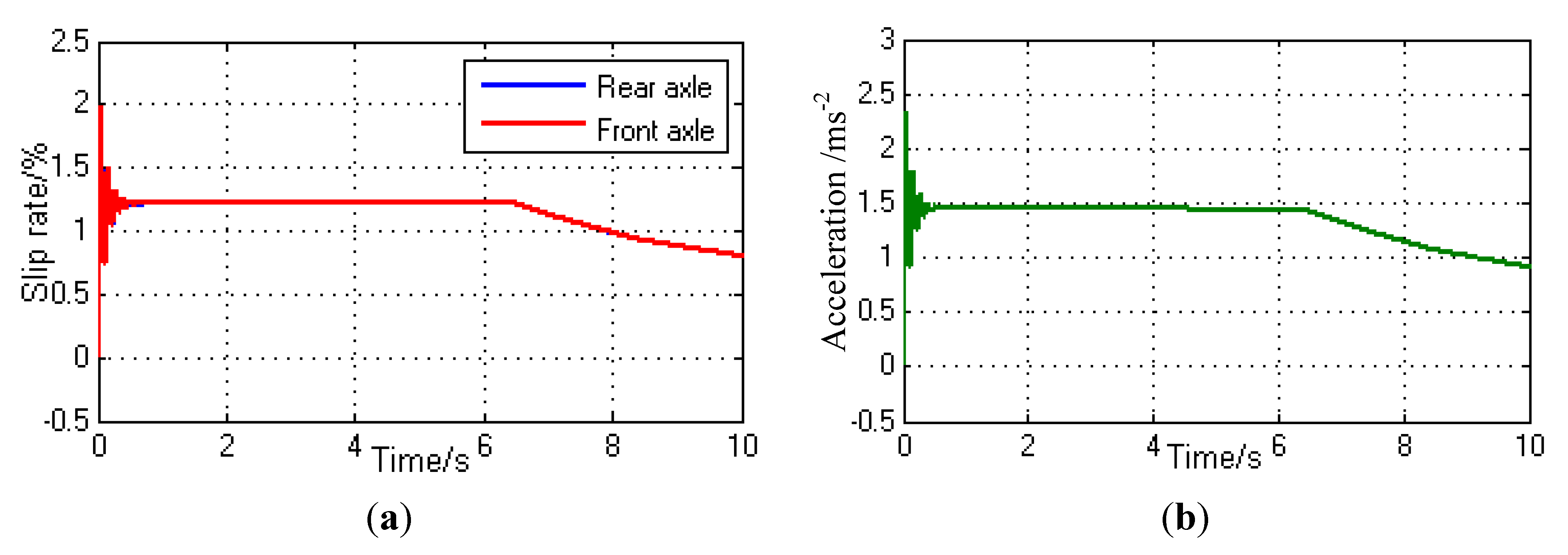
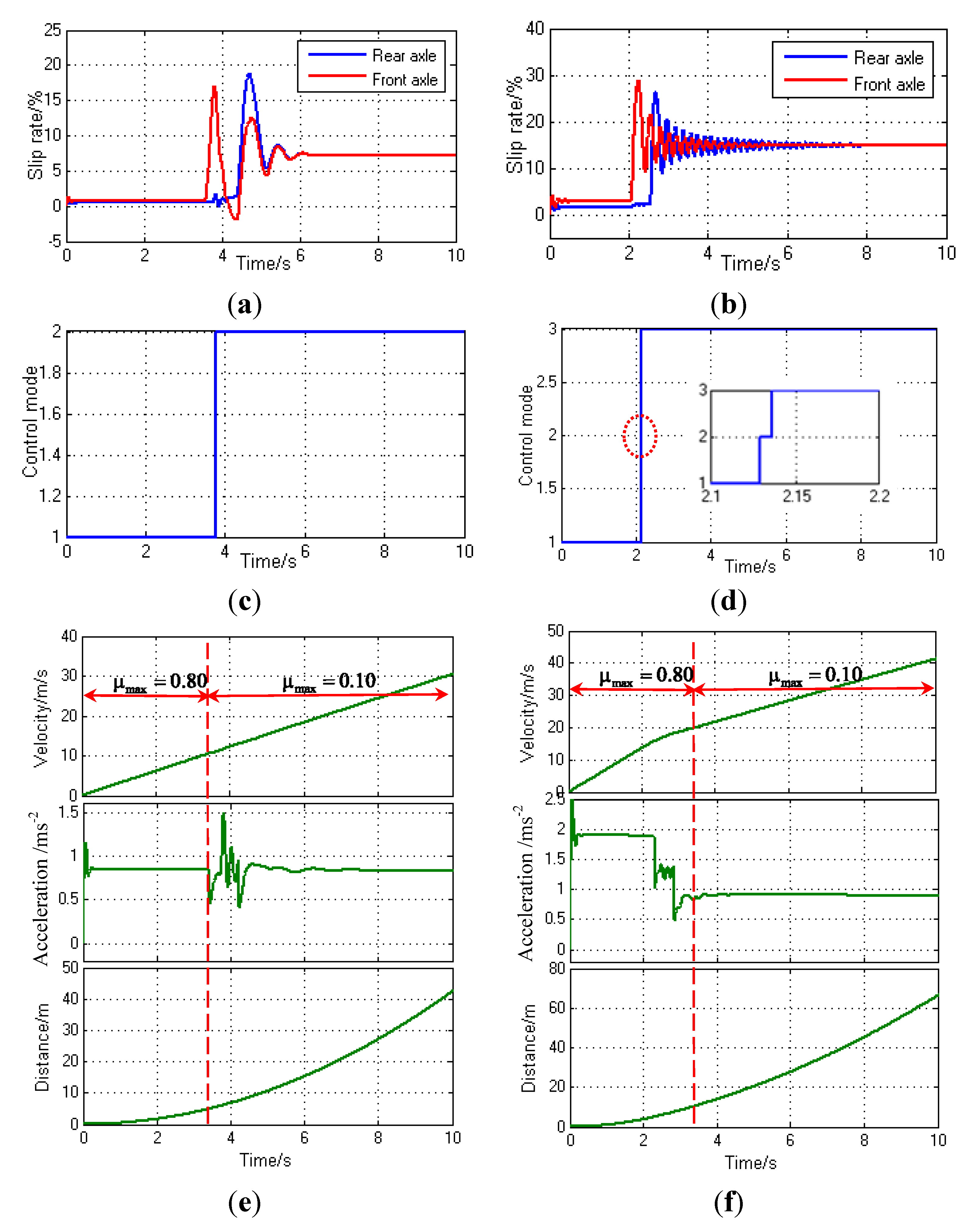
4.2. Simulation of Optimal Distribution of Inter-Axle Torque

When the driver steps on the acceleration pedal lightly on a mid-adhesion road, although the driver demanded torque is less than the total road adhesion at that time, if the average distribution of inter-axle torque control is still used, the drive axle which has the smaller axle load suffers a smaller ground tangential force, and the corresponding road adhesion is smaller, which may seriously slip due to its relatively large driving torque. Similarly, the drive axle which has smaller axle load has smaller road adhesion, and the corresponding drive torque is smaller, resulting in it being unable to take full advantage of the road adhesion conditions. Therefore, the design is based on an optimal distribution of inter-axle torque to have a reasonable distribution of the drive torque between the front and rear axles. The simulation results of slip rate between front and rear axle under the optimal distribution of inter-axle torque control and without torque control are shown in Figure 7, which shows the simulation results of the slip rate with control and without control for the driver accelerator pedal signal αpedal = 0.30 and peak road friction coefficient μH = 0.10.
Figure 7b shows that, if torque are distributed equally between the axles, the front axle with less axle load seriously slips, and the rear axle with large axle load maintains a slip rate λ = 5%, then the vehicle fails to make full use of the road adhesion for the axle. Figure 7a shows that after using the optimal distribution of inter-axle torque control, the slip rate of the front and rear axles remains the same in 0.5 s and the slip rate stabilized at around λ = 7.4% finally. Figure 7c,d are under the vehicle acceleration control corresponding to Figure 7a,b respectively, and in can be known that the vehicle acceleration is finally stabilized at 0.78 m/s2 under the optimal distribution of inter-axle torque control based on SMC (Slip Mode Control), while the vehicle acceleration eventually stabilizes at 0.65 m/s2 under the average torque distribution control. In poor road conditions, the optimal distribution of inter-axle torque control based on SMC was significantly better than the average torque distribution control, not only ensuring the vehicle’s longitudinal driving stability, but also improve the vehicle’s dynamic performance.
Figure 7. Simulation of stepping on the pedal lightly to accelerate on a mid-adhesion road: (a) Optimal torque of inter-axle distribution control; (b) Average torque distribution control; (c) Acceleration under optimal torque of the inter-axle distribution control; (d) Acceleration under the average torque distribution control.
Energies 07 03748 g007
The sliding mode control process under these conditions is shown in Figure 8. Figure 8a shows the change of the speed deviation of the front and rear axle tyres, and a deviation close to zero can be seen at around 0.4 s. Figure 8b shows the change of front and rear axle motor control torque output basically fluctuating at a stable value within ±10 Nm.
Figure 8. The change of sliding mode surface and controlled variables in the sliding mode control process: (a) Convergence process of the front and rear axle speed deviation; (b) Output torque of the front and rear axle motor under sliding mode control.
Energies 07 03748 g008

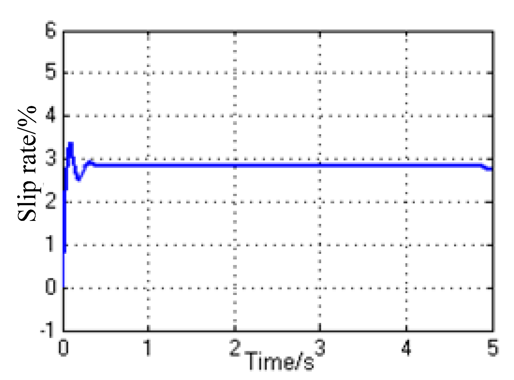
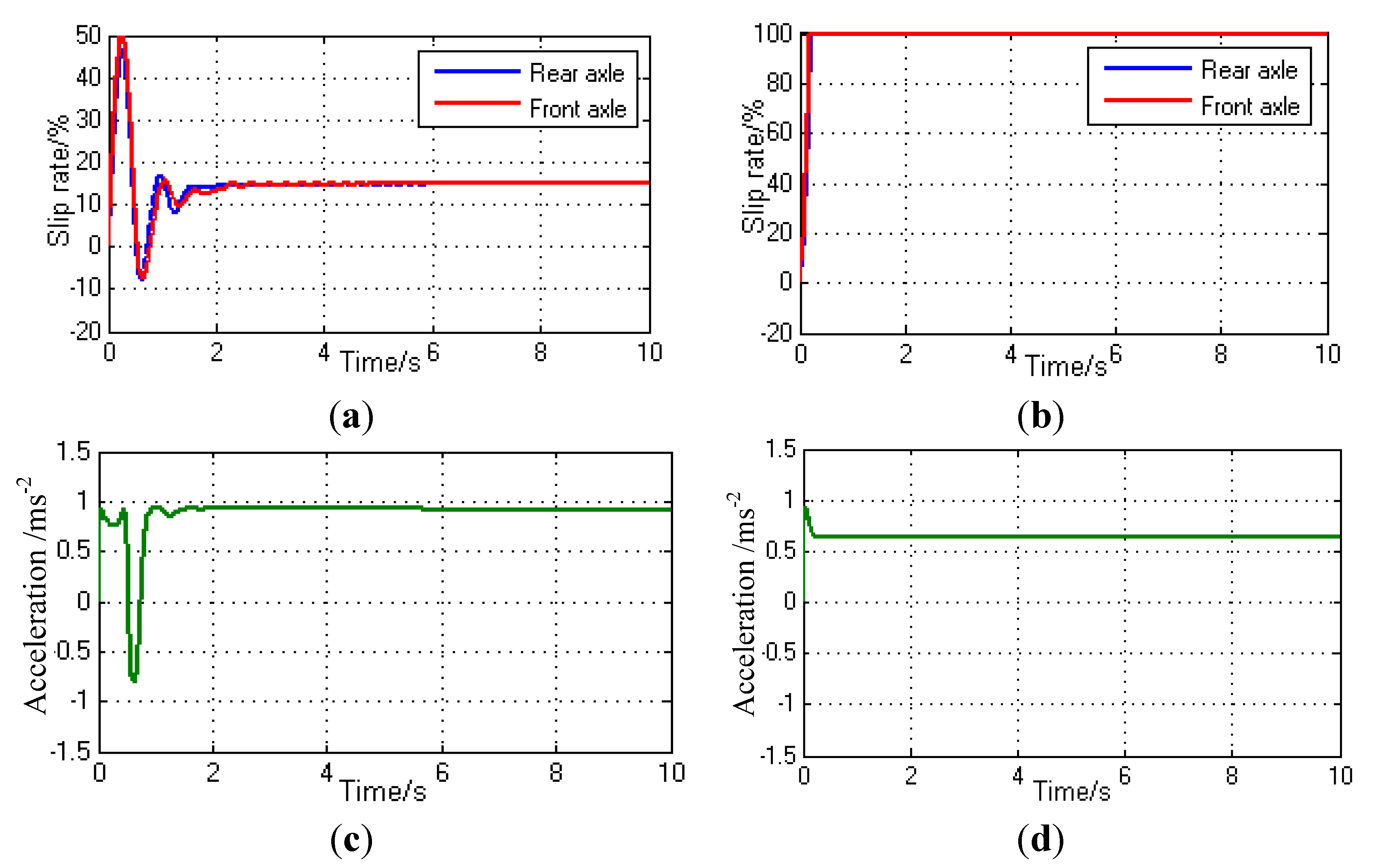
4.3. Simulation of Independent Control of Optimal Slip Rate

When the vehicle drives on s bad road and the driver-demanded torque is large, Tdesire > Troad, tyre slip can’t be avoided with the torque distribution between the axis based on optimal distribution of inter-axle torque control, so independent control of the optimal slip rate is required, the front and rear axle slip rate remains the best slip rate (referred to herein λopt = 15%), in order to fully use the road adhesion conditions and get maximum power. The signal of the driver accelerator pedal is set at αpedal = 0.8, and the peak road adhesion coefficient is set at μH = 0.10, and the independent control of optimal slip rate and the optimal distribution of inter-axle torque control results are shown in Figure 9.
Figure 9. Simulation results of stepping on the pedal heavily on snowy roads: (a) Independent control of the optimal slip rate; (b) Optimal distribution of inter-axle control; (c) Acceleration under independent control of optimal slip rate control; (d) Acceleration under optimal distribution of inter-axle torque control.
Energies 07 03748 g009
Figure 9b shows that the front and rear tyres seriously slip under optimal distribution of inter-axle torque control, the driver-demanded torque is much greater than road adhesion at this time, and the vehicle reaches an acceleration of 0.64 m/s2 in this mode, as shown in Figure 9d. As shown in Figure 9a, independent control of the optimal slip rate control can not only stabilize the front and rear axle tyres at the best slip point (λopt = 15%), but also maximize use of the road adhesion, to obtain an acceleration of 0.98 m/s2 which was shown in Figure 9c.
The front and rear axle independent control process under this condition is shown in Figure 10. Figure 10a,b are the deviation change of the drive axles tyres slip rate and optimum slip rate, respectively, which are basically within 0.4 s, the two axles tyres can be controlled in a stable slip area. Figure 10c shows front and rear axle output torque of the drive motor controls.
Figure 10. Front and rear axle input torque under different control modes: (a) Front axle slip rate control deviation; (b) Rear axle slip rate control deviation; (c) Output torque under independent control of the optimal slip rate mode.
Energies 07 03748 g010

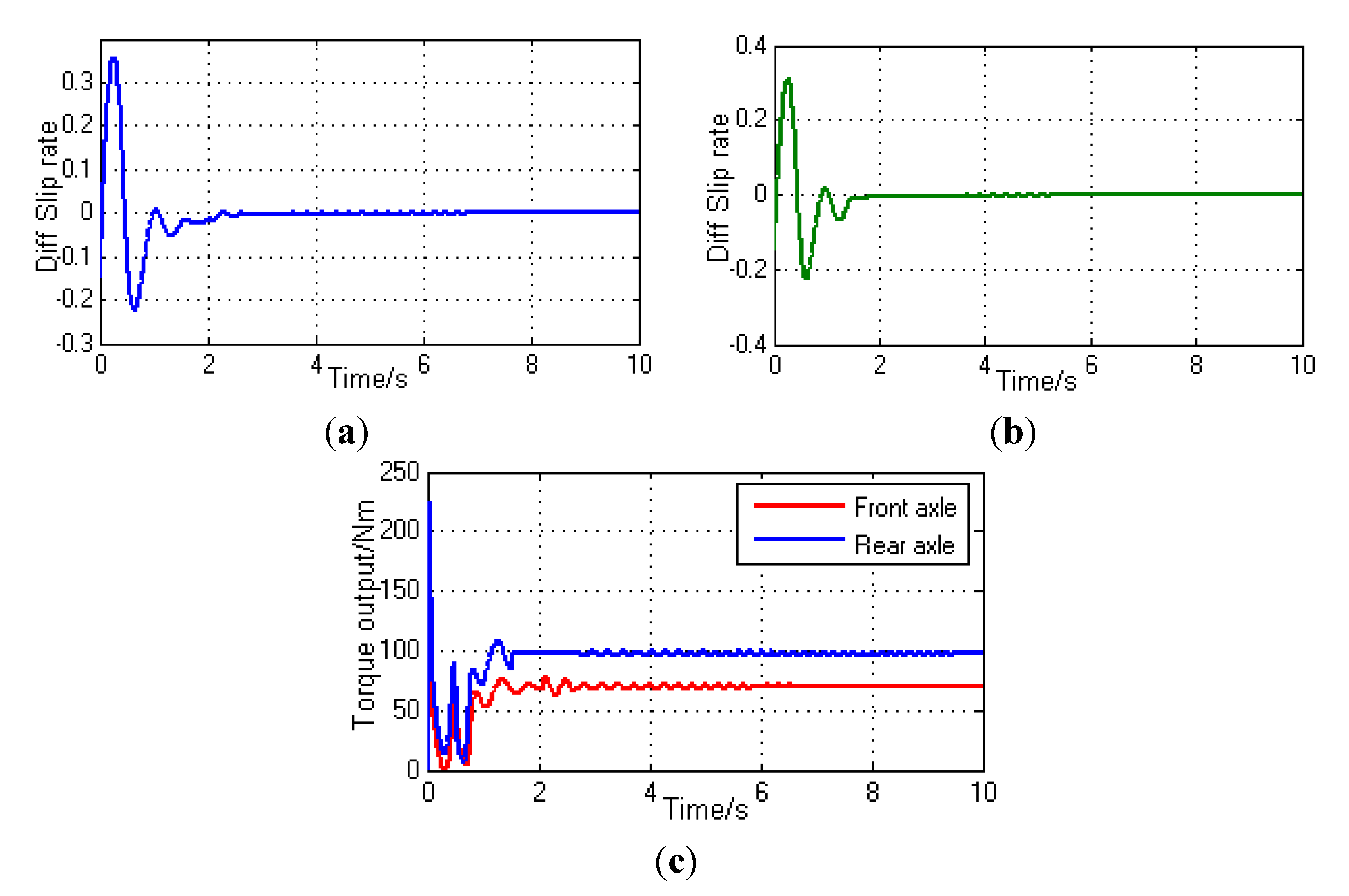
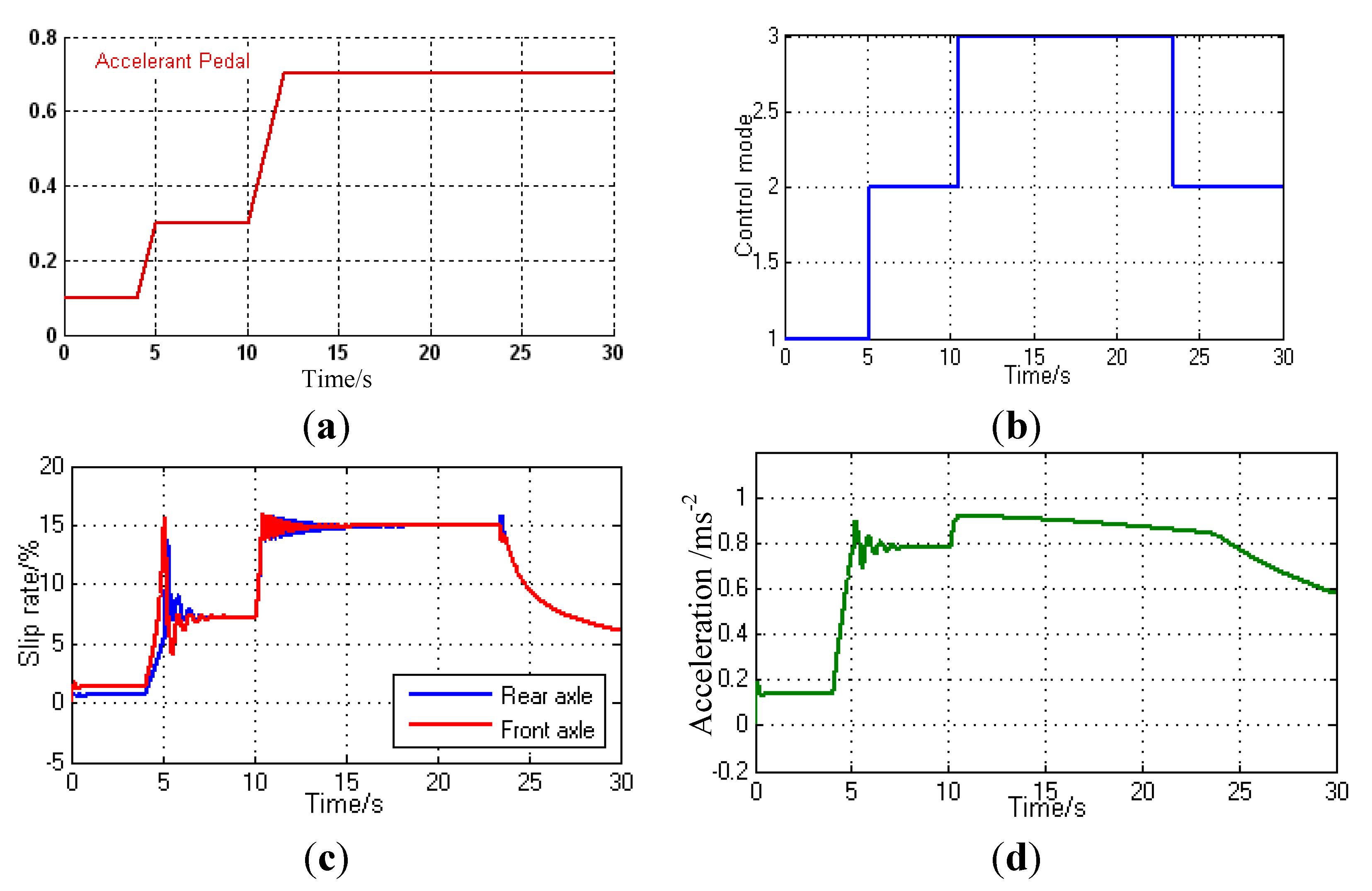
4.4. Comprehensive Simulation and Analysis of the Acceleration Slip Regulation Control Strategy

To further verify that the ASR control strategy can be effective for three different conditions to switch under constant driver-demanded torque, changing road conditions, and driver demanded torque changes, the road conditions remain unchanged to simulate two conditions. The simulation results are shown in Figure 11 and Figure 12. Where Figure 11c–f correspond to the vehicle driving characteristics under the conditions of Figure 11a,b, respectively.
Figure 11a shows that when the driver steps on the pedal lightly (αpedal = 0.3) by a dry road (μH = 0.80) to start with icy ground (μH = 0.10), at about 3.8 s the controller detects front axle tyre slip λ > 15%, so it switches the average distribution mode to the axis torque distribution based on SMC mode, as shown in Figure 11c, where “Control mode = 1” represents the conventional average torque distribution mode, “Control mode = 2” represents the axis torque distribution based on SMC mode, “Control mode = 3” represents front and rear axle independent control mode. Then under the optimal distribution of inter-axle torque control mode, the front and rear axle slip rate is basically the same at about 4.8 s, then it stabilizes at around 6 s. Since Tdesire < Troad is always correct, before the control mode switching, vehicle acceleration always follows the driver’s intention, steady at around 0.78 m/s2, as shown in Figure 11e.
Figure 11. Simulation results of torque distribution on changing roads: (a) Changes of slip rate with light pedal; (b) Changes of slip rate with heavy pedal; (c) Control mode switching; (d) Control mode switching; (e) Vehicle performance under light pedal; (f) Vehicle performance under heavy pedal.
Energies 07 03748 g011
Figure 11b shows that, when the driver steps on the pedal heavily (αpedal = 0.8) by a dry road ground (μH = 0.80) starting with icy ground (μH = 0.10), the controller detects that the front axle slips at about 2.1 s, mode switches from the average distribution of the torque to distribution of inter-axle torque, but Tdesire > Troad at this time, so distribution of inter-axle torque control is unable to prevent tyre slippage, so it continues to switch from distribution of inter-axle torque mode to the front and rear axles independent control mode, as shown in Figure 11d. Since Tdesire > Troad at this time, the front and rear axle independent control mode can take advantage of the road adhesion to the optimum dynamic, the acceleration eventually stabilizes at around 0.98 m/s2, as shown in Figure 11f.
To further verify the torque distribution strategy between the axis effective switching between the three control modes, we simulated under the same road conditions (μH = 0.10), the changing driver- demanded torque conditions, as shown in Figure 12.
Figure 12 shows that, when the vehicle is traveling on the icy road (αpedal = 0.1) with pedal signal αpedal = 0.1, the driver-demanded torque is small, the front and rear drive axles are both under road adhesion conditions, and the controller controls the front and rear axle drive motors under average torque distribution mode. Then at about 4 s, the pedal changes to αpedal = 0.3, then the slip rate of the front axle has a slip trend, and then the controller switches to the axis torque distribution based on SMC mode. When the pedal depth further increases until αpedal = 0.8, the total ground adhesion is not enough, so slippage can’t be avoided by torque distribution between the axles, so the controller switches to the front and rear axles independent control mode. With increasing speed, the motor transforms from constant torque region to constant power region, under the constant accelerator pedal, the driver-demanded torque is decreasing, then the mode switches to “the axis torque distribution based on SMC mode” again, as shown in Figure 12b with the oval label. Figure 12d shows the change of vehicle acceleration under these conditions, and the vehicle dynamics can follow the driver’s intentions well.
It can thus be seen that the proposed inter-axis torque distribution control strategy can effectively switch between different conditions, ensuring the vehicle dynamics while improving the vehicle's longitudinal driving stability.
Figure 12. Simulation results under the same road with the changing driver accelerator pedal: (a) Driver accelerator pedal signal; (b) The change of control mode under inter-axle torque distribution control strategy; (c) Change of slip rate; (d) Vehicle acceleration.
Energies 07 03748 g012

5. Conclusions

(1)
Aiming at the 4WD electric vehicle, which was driven by front and rear independent motors, a model of the ASR system was established.
(2)
Compared with the conventional method of slip rate calculation, using the state equation of slip rate can be more accurate to describe the tyre slip process in a low vehicle velocity situation.
(3)
An ASR control strategy which contains three torque distribution mode was designed, namely average distribution of inter-axle torque for high road adhesion, optimal distribution of inter-axle torque for middle road adhesion and independent control of optimal slip rate for low road adhesion. Several simulations were carried out with MATLAB/Simulink, and the simulation results with some comparisons show that, the proposed strategy could realize the transformation among different control modes, thus fully use the road adhesion conditions, make the vehicle’s dynamic performance to follow the driver’s wishes. As a result, the vehicle longitudinal drive stability and dynamic performance are ensured.

Acknowledgments

This work was supported by the National High Technology Research and Development Program of China (2012AA111603, 2013BAG05B00) in part, the Program for New Century Excellent Talents in University (NCET-11-0785) and Beijing Institute of Technology Post Graduate Students Innovation Foundation in part. The author would also like to thank the reviewers for their corrections and helpful suggestions.

Author Contributions

Hongwen He and Jiankun Peng built the dynamic model of ASR for 4WDEV and performed the simulations, Rui Xiong designed the control modes, Hao Fan debugged the algorithm. All authors carried out data analysis, discussed the results and contributed to writing the paper.

Conflicts of Interest

The authors declare no conflict of interest.

References

  1. Wang, J.; Wang, Q.; Jin, L.; Song, C. Independent wheel torque control of 4WD electric vehicle for differential drive assisted steering. Mechatronics 2011, 21, 63–76. [Google Scholar] [CrossRef]
  2. Kang, J.; Yoo, J.; Yi, K. Driving control algorithm for maneuverability, lateral stability, and rollover prevention of 4WD electric vehicles with independently driven front and rear wheels. IEEE Trans. Veh. Technol. 2011, 60, 2987–3001. [Google Scholar] [CrossRef]
  3. Dasgupta, K. Analysis of a hydrostatic transmission system using low speed high torque motor. Mech. Mach. Theory 2000, 35, 1481–1499. [Google Scholar] [CrossRef]
  4. Gasbaoui, B.; Nasri, A. A Novel 4WD Electric Vehicle Control Strategy Based on Direct Torque Control Space Vector Modulation Technique. Intell. Control. Autom. 2012, 3, 236–242. [Google Scholar] [CrossRef]
  5. Xue, X.; Cheng, K.; Ng, T.; Cheung, N.C. Multi-objective optimization design of in-wheel switched reluctance motors in electric vehicles. IEEE Trans. Ind. Electron. 2010, 57, 2980–2987. [Google Scholar] [CrossRef]
  6. Tong, Q. Simulation Study on the Longitudinal Dynamics of a Full Drive Vehicle with Two Separated Motors. Master’s Thesis, Beijing Institute of Technology, Beijing, China, 2013. [Google Scholar]
  7. Jalali, K.; Uchida, T.; McPhee, J.; Lambert, S. Development of a Fuzzy Slip Control System for Electric Vehicles with In-wheel Motors. SAE Int. J. Altern. Powertrains 2012, 1, 46–64. [Google Scholar]
  8. Liu, W.; He, H.; Peng, J. Driving Control Research for Longitudinal Dynamics of Electric Vehicles with Independently Driven Front and Rear Wheels. Math. Probl. Eng. 2013, 2013. [Google Scholar] [CrossRef]
  9. Zhao, Z. Study of acceleration slip regulation strategy for four wheel drive hybrid electric car. Chin. J. Mech. Eng. 2011, 47, 83–98. [Google Scholar] [CrossRef]
  10. Sakai, S.; Hori, Y. Advantage of electric motor for anti-skid control of electric vehicle. Eur. Power Electron. Drives J. 2001, 11, 26–32. [Google Scholar]
  11. Yin, D.; Oh, S.; Hori, Y. A novel traction control for EV based on maximum transmissible torque estimation. IEEE Trans. Ind. Electron. 2009, 56, 2086–2094. [Google Scholar] [CrossRef]
  12. Chen, F.W.; Liao, T.L. Nonlinear linearization controller and genetic algorithm based fuzzy logic controller for ABS systems and their comparison. Int. J. Veh. Des. 2000, 24, 334–349. [Google Scholar] [CrossRef]
  13. Nakakuki, T.; Shen, T.; Tamura, K. Adaptive control approach to uncertain longitudinal tire slip in traction control of vehicles. Asian J. Control. 2008, 10, 67–73. [Google Scholar] [CrossRef]
  14. Liu, J.K. Sliding Mode Control Design and MATLAB Simulation, 2nd ed.; Tsinghua University Press: Beijing, China, 2012. [Google Scholar]
  15. Ameodeo, M.; Ferrara, A.; Terzaghi, R.; Vecchio, C. Wheel Slip Control via Second–Order Sliding-Model Generation. IEEE Trans. Intell. Trans. Syst. 2010, 11, 122–131. [Google Scholar] [CrossRef]
  16. Bashash, S.; Fathy, H.K. Transport-based load modeling and sliding mode control of plug-in electric vehicles for robust renewable power tracking. IEEE Trans. Smart Grid 2012, 3, 526–534. [Google Scholar] [CrossRef]
  17. Subudhi, B.; Ge, S.S. Sliding-Mode-Observer-Based Adaptive Slip rate Control for Electric and Hybrid Vehicles. IEEE Trans. Intell. Trans. Syst. 2012, 13, 1617–1626. [Google Scholar] [CrossRef]
  18. Kim, J.; Park, C.; Hwang, S.; Hori, Y. Control algorithm for an independent motor-drive vehicle. IEEE Trans. Veh. Technol. 2010, 59, 3213–3222. [Google Scholar] [CrossRef]
  19. Austin, L.; Morrey, D. Recent advances in antilock braking systems and traction control systems. Proc. Inst. Mech. Eng. Part D 2000, 214, 625–638. [Google Scholar] [CrossRef]
  20. Peng, J.K.; He, H.W.; Feng, N.L. Simulation Research on an Electric Vehicle Chassis System Based on a Collaborative Control System. Energies 2013, 6, 312–328. [Google Scholar] [CrossRef]
  21. Pacejka, H.B.; Bakker, E. The magic formula tyre model. Veh. Syst. Dyn. 1992, 21, 1–18. [Google Scholar] [CrossRef]
  22. Clover, C.; Bernard, J. Longitudinal tire dynamics. Veh. Syst. Dyn. 1998, 29, 231–260. [Google Scholar] [CrossRef]

