Novel Modeling and Control Strategies for a HVAC System Including Carbon Dioxide Control

Abstract

Conventional heating, ventilating, and air conditioning (HVAC) systems have traditionally used the temperature and the humidity ratio as the quantitative indices of comfort in a room. Recently, the carbon dioxide (CO₂) concentration has also been recognized as having an important contribution to room comfort. This paper presents the modeling of an augmented HVAC system including CO₂ concentration, and its control strategies. Because the proposed augmented HVAC system is multi-input multi-output (MIMO) and has no relative degree problem, the dynamic extension algorithm can be employed; then, a feedback linearization technique is applied. A linear-quadratic regulator (LQR) is designed to optimize control performance and to stabilize the proposed HVAC system. Simulation results are provided to validate the proposed system model, as well as its linearized control system.

1. Introduction

HVAC systems are automatic systems that control temperature and humidity in buildings, providing people with a comfortable environment. The use of HVAC systems represents more than 50% of the world energy consumption [1,2,3,4]. Thus, balancing occupant comfort and energy efficiency is a main goal of HVAC control strategies.

In most previous studies, HVAC systems have been modeled considering only the temperature and the humidity ratio [5,6,7,8]. A nonlinear HVAC model that includes dynamics of temperature and humidity ratio is proposed in [5], which includes the design of an observer to estimate the thermal and moisture loads. In [6], an adaptive fuzzy output feedback controller is proposed, based on an observer for the HVAC system. In [7,8], a back-stepping controller and a decentralized nonlinear adaptive controller are respectively applied to the same model.

Recently, the CO₂ concentration has been recognized as having an important contribution to room comfort [9,10]. Some researchers have proposed hybrid HVAC systems that represent the temperature and humidity ratio as continuous states and CO₂ concentration as a discrete state [11,12]. However, because these states are strongly interrelated, it is more appropriate to integrate these continuous and discrete dynamics into a single model that includes temperature, humidity ratio, and CO₂ concentration as states.

This paper presents a modeling and control strategy for a novel HVAC system that considers temperature, humidity ratio, and CO₂ concentration. In the process of modeling, the dynamic extension algorithm of [13] is employed to deal with non-interacting control problem and no relative degree problem. After the dynamic extension process, a feedback linearization method can be applied to the proposed HVAC system to convert a bilinear system into a linear system. Linear controllers, pole placement and LQR can be designed for the linearized novel HVAC system to stabilize it and improve its control performance.

This paper is organized as follows: in Section 2, we present the bilinear model for the conventional HVAC system, including valve dynamics. Section 3 presents a novel HVAC system including CO₂ concentration and its applicability in the feedback linearization method. Also, dynamic extension algorithm is applied for solving the no relative degree and interacting control problems in the MIMO system. In Section 4, we describe the design of linear controllers for the linearized HVAC system, such as pole placement and LQR controllers, to improve the system’s control performance and to verify the effectiveness of the proposed model.

2. Conventional HVAC System with Temperature and Humidity Ratio

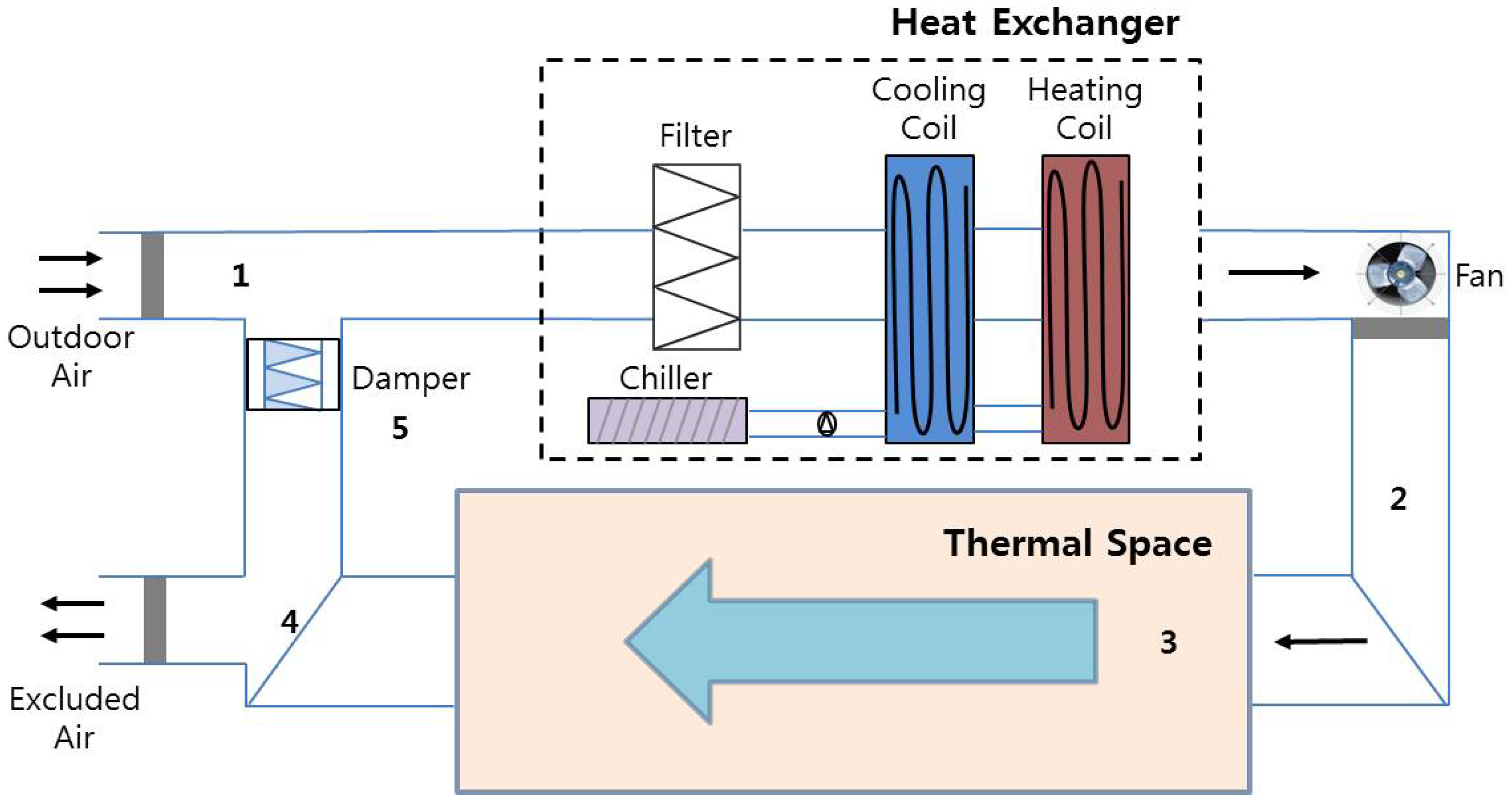
As mentioned, conventional HVAC systems control only temperature and humidity. In this paper, we consider the single-zone system shown in Figure 1 as a representative conventional HVAC system. It consists of the following components: a heat exchanger; a chiller, which provides chilled water to the heat exchanger; a circulating air fan; the thermal space; connecting ductwork; dampers; and mixing air components [5]. The conventional HVAC system controls the temperature and humidity ratio as follows [5]:

• Fresh air is introduced into the system and is mixed in a 25:75 ratio with recirculated air (position 5) at the flow mixer.
• Second, air mixed at the flow mixer (position 1) enters the heat exchanger, where it is conditioned.
• Third, the conditioned air is moved out of the heat exchanger; this air is ready to enter the thermal space, and is called supply air (position 2).
• Fourth, the supply air enters the thermal space (position 3), where it offsets the sensible (actual heat) and latent (humidity) heat loads acting upon the system.
• Finally, the air in the thermal space is drawn through a fan (position 4); 75% of this air is recirculated and the rest is exhausted from the system.

Figure 1. Model of the representative conventional HVAC system.

Figure 1. Model of the representative conventional HVAC system.

The control inputs for a conventional HVAC system are the flow rate of air, which is varied using a variable-speed fan (position 2), and the flow rate of water from the chiller to the heat exchanger. However, in our proposed HVAC system, the air recirculation rate (position 4) is added as a new control input, and some modifications are made to the basic operation rules listed above. That is to say, the 75% recirculation rate listed above in the first and last steps becomes a variable quantity, and is used as the third control input.

2.1. Mathematical Modeling of Conventional HVAC System

The conventional HVAC system is a model considering the temperature and the humidity ratio as states. The differential equations describing the dynamic behavior of the HVAC system in Figure 1 can be derived from energy conservation principles and are given by [5]:

(1)

The dynamic system given by Equation (1) can be converted into a state variable form for the purposes of control. Let $u_1=F$, $u_2=gpm$, $z_1=T_3$, $z_2=W_3$, $z_3=T_2$ and define the following parameters: ${\alpha }_1=\frac{60}{V_s}$, ${\alpha }_2=\frac{60h_{fg}}{C_p{V}_s}$, ${\alpha }_3=\frac{1}{{\rho }_a{C}_p{V}_s}$, ${\alpha }_4=\frac{1}{{\rho }_a{V}_s}$, ${\beta }_1=\frac{60}{V_{he}}$, ${\beta }_2=\frac{1}{{\rho }_a{C}_p{V}_{he}}$, and ${\beta }_3=\frac{60h_w}{C_p{V}_{he}}$. Then, the dynamic equations given in Equation (1) can be written in the following state variable form.

(2)

The conventional HVAC system of Equation (2) is a 2-input, 2-output MIMO system: its inputs are the volumetric air flow rate and the chilled water flow rate, and its outputs are the temperature and the humidity ratio of the thermal space.

2.2. Adding Valve Dynamics to the Conventional HVAC Model

The Control input signals $u={\left[u_1{u}_2\right]}^T$ in the system described in Equation (2) are implemented using liquid valves. The valve dynamics can be modeled as follows in which $\psi \left(\text{s}\right)$ is the valve inherent characteristic and $u\left(s\right)$ is the flow rate of the liquid which enters the valve [14,15]:

$$u\left(s\right)=\frac{1}{\left(1+\tau s\right)}\psi \left(\text{s}\right)$$

(3)

By considering the characteristic of a linear valve as $\psi \left(\text{s}\right)=kv\left(s\right)$, the valve transfer function can be written as:

$$u_1=\frac{k_1}{1+{\tau }_{1}s}{\nu }_1\text{, }{u}_2=\frac{k_2}{1+{\tau }_{2}s}{\nu }_2$$

(4)

where $k_1$$k_2$${\tau }_1$ and ${\tau }_2$ are the constant gains and the time constants, respectively; $\nu ={\left[{\nu }_1{\nu }_2\right]}^T$ is the control signal applied to the actuator; and $u={\left[u_1{u}_2\right]}^T$ is the signal that is input to the HVAC system.

An augmented state space model with the new state vector, $z={\left[z_1{z}_2{z}_3{u}_1{u}_2\right]}^T={\left[z_1{z}_2{z}_3{z}_4{z}_5\right]}^T$ can be derived as:

$$\{\begin{array}{c}\dot{z}=f\left(z\right)+g\left(z\right)\nu = \left[\begin{array}{c}{a}_1\left(z\right)\\ \begin{array}{c}{a}_2\left(z\right)\\ a_3\left(z\right)\\ a_4(z)\end{array}\\ a_5\left(z\right)\end{array}\right]+\left[\begin{array}{cc}0& 0\\ \begin{array}{c}0\\ 0\\ \frac{k_1}{{\tau }_1}\\ 0\end{array}& \begin{array}{c}0\\ 0\\ 0\\ \frac{k_2}{{\tau }_2}\end{array}\end{array}\right]\nu \\ y=\left[z_1 z_2\right]{ }^T\end{array}$$

(5)

where:

Thus, the system in Equation (5) represents a conventional HVAC system to which valve dynamics have been applied to implement the control signals. This conventional system can regulate only the temperature and the humidity ratio; other factors such as CO₂ concentration, which affects the health of occupants or workers indoors, cannot be considered.

3. Novel Modeling of HVAC System including CO₂ Concentration

If the recirculated air contains too much CO₂, it can affect the health and work efficiency of the building’s occupants. Therefore, CO₂ concentration should be one of the quantitative indices of room comfort, along with temperature and humidity ratio. In this paper, we propose an HVAC system that continuously controls all three of these indices.

From the mass balance equation, the average CO₂ concentration $C_s$ in the room can be represented as [14]:

$$V_s{\dot{C}}_s=C_g+\left(1-\mu \right)\left(C_i-C_o\right)$$

(6)

where $C_s=C_i-C_o$, $C_g$ is the amount of CO₂ generated in the room; $C_i$ is the CO₂ concentration in the inlet air; $C_o$ is the CO₂ concentration of air leaving the room, and $\left(1-\mu \right),0\le \mu \le 1$, is the air exchange rate.

3.1. Proposed HVAC System Model

The proposed HVAC system model includes CO₂ concentration as a state. The differential Equation (6) can be integrated into the dynamic equations in (1). The valve dynamics of $u_3$ are added to the control input vector $u={\left[u_1{u}_2\right]}^T$, and the control signal applied to the actuator of ${\nu }_3$ also can be added to the actuator input vector $\nu$.

Let $u_3=1-\mu$, ${\text{x}}_1=z_1$, ${\text{x}}_2=z_2$, ${\text{x}}_3=z_3$, ${\text{x}}_4=C_s$, and let an augmented state vector $x={\left[{\text{x}}_1{\text{x}}_2{\text{x}}_3{\text{x}}_4{u}_1{u}_2{u}_3\right]}^T$. Then, the whole dynamics can be written in the state variable form as:

(7)

where:

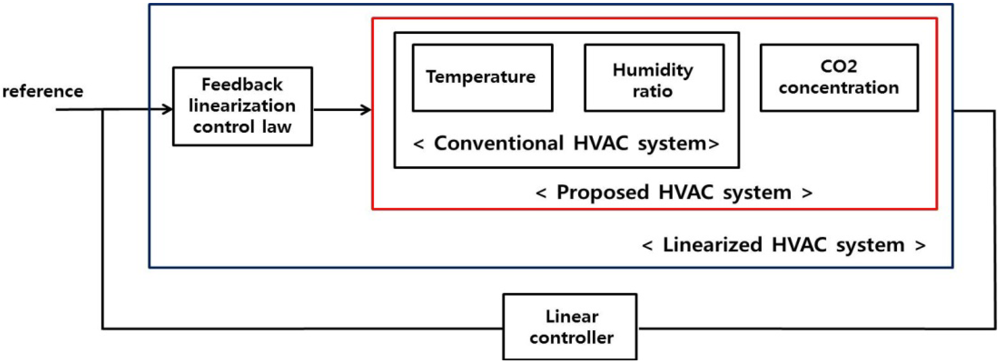
The novel HVAC system of (7) is a 3-input, 3-output MIMO system: its inputs are the volumetric air flow rate, the chilled water flow rate, and the outdoor air flow rate, and its outputs are the temperature, humidity ratio, and CO₂ concentration of the thermal space. This proposed HVAC system can be linearized using a feedback linearization control method, as shown in Figure 2. Thus, we can finally obtain a linearized HVAC system that can be controlled using linear controllers.

Figure 2. Overall block diagram for controlling the proposed HVAC system.

Figure 2. Overall block diagram for controlling the proposed HVAC system.

3.2. Conditions for Input-Output Feedback Linearization

An input-output feedback linearization method can be applied to the state space model given in (7) to track the desired temperature, humidity ratio, and CO₂ concentration only when the decoupling matrix is non-singular. However, the decoupling matrix (refer to Appendix A2):

$$D\left(x\right)=\left[\begin{array}{ccc}{L}_{g_1}{L}_f^1{\text{x}}_1& L_{g_2}{L}_f^1{\text{x}}_1& L_{g_3}{L}_f^1{\text{x}}_1\\ L_{g_1}{L}_f^1{\text{x}}_2& L_{g_2}{L}_f^1{\text{x}}_2& L_{g_3}{L}_f^1{\text{x}}_2\\ L_{g_1}{L}_f^1{\text{x}}_4& L_{g_2}{L}_f^1{\text{x}}_4& L_{g_3}{L}_f^1{\text{x}}_4\end{array}\right]=\left[\begin{array}{ccc}\frac{{\gamma }_1{k}_1}{{\tau }_1}& 0& 0\\ \frac{{\gamma }_2{k}_1}{{\tau }_1}& 0& 0\\ 0& 0& \frac{{\gamma }_5{k}_3}{{\tau }_3}\end{array}\right]$$

is singular; here, $L\left(\bullet \right)$ represents the Lie derivative and the total relative degree is $6\ne \text{n}$, where $\text{n}$ is the system order [16]. When the invertibility condition is violated, some method is needed to carry out an input-output linearization; the dynamic extension algorithm used herein is such a method.

3.2.1. Dynamic Extension Algorithm

Because input-output linearization can be achieved only when the decoupling matrix $D\left(x\right)$ is non-singular, employing the dynamic extension algorithm involves choosing some new inputs that are the derivatives of some of the original system inputs, in such a way that the decoupling matrix $D\left(x\right)$ becomes non-singular, as shown in Figure 3 [16].

Figure 3. Concept of the dynamic extension algorithm [13].

Figure 3. Concept of the dynamic extension algorithm [13].

Let state vector $\stackrel{-}{x}={\left[x{v}_1{v}_3\right]}^T={\left[{\text{x}}_1{\text{x}}_2{\text{x}}_3{\text{x}}_4{u}_1{u}_2{u}_3{v}_1{v}_3\right]}^T$. Then, the state space can be written as:

(8)

where:

The decoupling matrix as changed by the dynamic extension (refer to Appendix A3):

is non-singular. The vector relative degree is $\left\{\begin{array}{ccc}3& 3& 3\end{array}\right\}$ and and the total relative degree is equal to the system order $\text{n}$, which means that there are no internal dynamics [16]. Therefore, we can achieve relative degree and non-interacting control.

3.3. Equivalent Linearization HVAC System

To be able to apply the feedback linearization method conveniently, we can change system (8) into the equivalent system (9) by using Equation (A3):

$$\{\begin{array}{c}{\dot{x}}^{\prime }=A{x}^{\prime }+B\left[F\left(x^{\prime }\right)+G\left(x^{\prime }\right)\zeta \right]\\ y={\left[\begin{array}{ccc}{y}_1& y_2& y_3\end{array}\right]}^T={\left[\begin{array}{ccc}{\text{x}}_1& {\text{x}}_2& {\text{x}}_4\end{array}\right]}^T\end{array}$$

(9)

where:

$$x^{\prime }={\left[{\text{x}}_1{\text{x}}_1^{\left(1\right)}{\text{x}}_1^{\left(2\right)}{\text{x}}_2{\text{x}}_2^{\left(1\right)}{\text{x}}_2^{\left(2\right)}{\text{x}}_4{\text{x}}_4^{\left(1\right)}{\text{x}}_4^{\left(2\right)}\right]}^T\text{;}$$

$$F\left(x^{\prime }\right)={\left[f_1{f}_2{f}_3\right]}^T\text{;}$$

$$G\left(x^{\prime }\right)=\left[\begin{array}{ccc}{g}_{11}& g_{12}& g_{13}\\ g_{21}& g_{22}& g_{23}\\ g_{31}& g_{32}& g_{33}\end{array}\right]\text{;}$$

$$A=diag\left[\begin{array}{ccc}\left[\begin{array}{ccc}0& 1& 0\\ 0& 0& 1\\ 0& 0& 0\end{array}\right]& \left[\begin{array}{ccc}0& 1& 0\\ 0& 0& 1\\ 0& 0& 0\end{array}\right]& \left[\begin{array}{ccc}0& 1& 0\\ 0& 0& 1\\ 0& 0& 0\end{array}\right]\end{array}\right]\text{;}$$

$$B=diag\left[\begin{array}{ccc}\left[\begin{array}{c}0\\ 0\\ 1\end{array}\right]& \left[\begin{array}{c}0\\ 0\\ 1\end{array}\right]& \left[\begin{array}{c}0\\ 0\\ 1\end{array}\right]\end{array}\right]\text{;}$$

and $C=\text{diag}\left[\begin{array}{ccc}\left[\begin{array}{ccc}1& 0& 0\end{array}\right]& \left[\begin{array}{ccc}1& 0& 0\end{array}\right]& \left[\begin{array}{ccc}1& 0& 0\end{array}\right]\end{array}\right]$.

This equivalent system can apply the feedback linearization law to linearize the HVAC system. By putting proper control gain, the linearized HVAC system can be regulated to maintain the set points of temperature, humidity ratio, and CO₂ concentration.

4. Control Strategies Using Feedback Linearization Control

The proposed HVAC system is linearized by a feedback linearization method. The linearized HVAC system shown can be controlled by linear controllers such as pole placement and LQR controllers.

Table 1 shows the numerical values of system parameters used in the simulations. The initial state and reference values are given in Table 2.

Table 1. Numerical values for system parameters.

Parameter	Value	Unit
ρ	0.074	1b/ft3
Vhe	60.75	ft3
Vs	58464	ft3
Cp	0.24	Btu/lb °F
Ws	0.0070	lb/lb
Mo	166.06	lb/hour
Qo	289,897.52	Btu/hour
To	85	°F
Wo	0.018	1b/1b
Co	400	ppm
τ1,τ2,τ3	0.008	hour
k1,k2,k3	5	-

Table 1. Numerical values for system parameters.

Parameter	Value	Unit
ρ	0.074	1b/ft3
Vhe	60.75	ft3
Vs	58464	ft3
Cp	0.24	Btu/lb °F
Ws	0.0070	lb/lb
Mo	166.06	lb/hour
Qo	289,897.52	Btu/hour
To	85	°F
Wo	0.018	1b/1b
Co	400	ppm
τ1,τ2,τ3	0.008	hour
k1,k2,k3	5	-

Table 2. Initial state and reference values.

Tinitial	76 °F	Tinitial	0.021 lb/lb	Tinitial	1300ppm
Tinitial	71 °F	Tinitial	0.0092 lb/lb	Tinitial	1200ppm

Table 2. Initial state and reference values.

Tinitial	76 °F	Tinitial	0.021 lb/lb	Tinitial	1300ppm
Tinitial	71 °F	Tinitial	0.0092 lb/lb	Tinitial	1200ppm

4.1. Design of Pole Placement Control for Linearized HVAC System

Let the reference signal $y_d={\left[\begin{array}{ccc}{y}_{1d}& y_{2d}& y_{3d}\end{array}\right]}^T$, $y_d^{\left(3\right)}={\left[\begin{array}{ccc}{y}_{1d}^{\left(3\right)}& y_{2d}^{\left(3\right)}& y_{3d}^{\left(3\right)}\end{array}\right]}^T$, and matrix $Y_d={\left[\begin{array}{ccc}{y}_{1d}& y_{1d}^{\left(1\right)}& y_{1d}^{\left(2\right)}\end{array}\begin{array}{ccc}{y}_{2d}& y_{2d}^{\left(1\right)}& y_{2d}^{\left(2\right)}\end{array}\begin{array}{ccc}{y}_{3d}& y_{3d}^{\left(1\right)}& y_{3d}^{\left(2\right)}\end{array}\right]}^T$. Define the tracking errors as ${\text{e}}_1=y_1-y_{1d}$, ${\text{e}}_2=y_2-y_{2d}$ and ${\text{e}}_3=y_3-y_{3d}$, and let the error matrix $e=x^{\prime }-Y_d={\left[e_1{e}_1^{\left(1\right)}{e}_1^{\left(2\right)}{e}_2{e}_2^{\left(1\right)}{e}_2^{\left(2\right)}{e}_3{e}_3^{\left(1\right)}{e}_3^{\left(2\right)}\right]}^T$.

The feedback linearization control law for the proposed HVAC system (9) is designed as:

$$\zeta =G^{-1}\left(-F+y_d^{\left(3\right)}-Ke\right)$$

(10)

choosing $K=\text{diag}\left(\left[\begin{array}{ccc}{k}_{11}& k_{12}& k_{13}\end{array}\right],\left[\begin{array}{ccc}{k}_{21}& k_{22}& k_{23}\end{array}\right],\left[\begin{array}{ccc}{k}_{31}& k_{32}& k_{33}\end{array}\right]\right)$ so that the polynomial $s^3+k_{i1}{s}^2+k_{i2}{s}^1+k_{i3}=0,i=1,2,3$ has all its roots strictly in the left-half complex plane, thereby meeting the desired performance specifications such as those for the transient response of the steady-state error. By substituting Equation (10) into Equation (9), the linearized HVAC system can finally be obtained as follows:

$${\dot{x}}^{\prime }=A{x}^{\prime }+B\eta$$

(11)

where $\eta =y_d^{\left(3\right)}-Ke$.

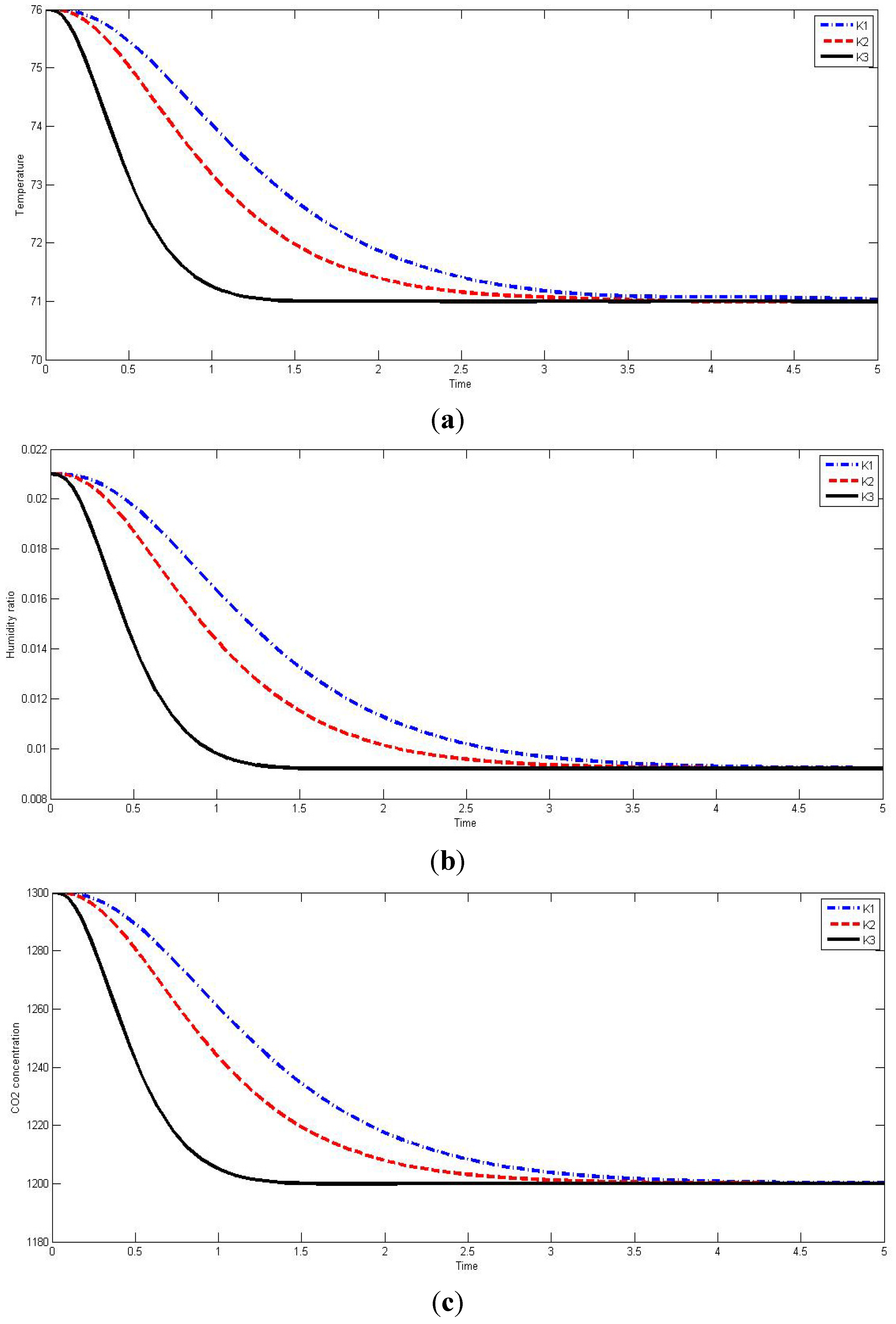
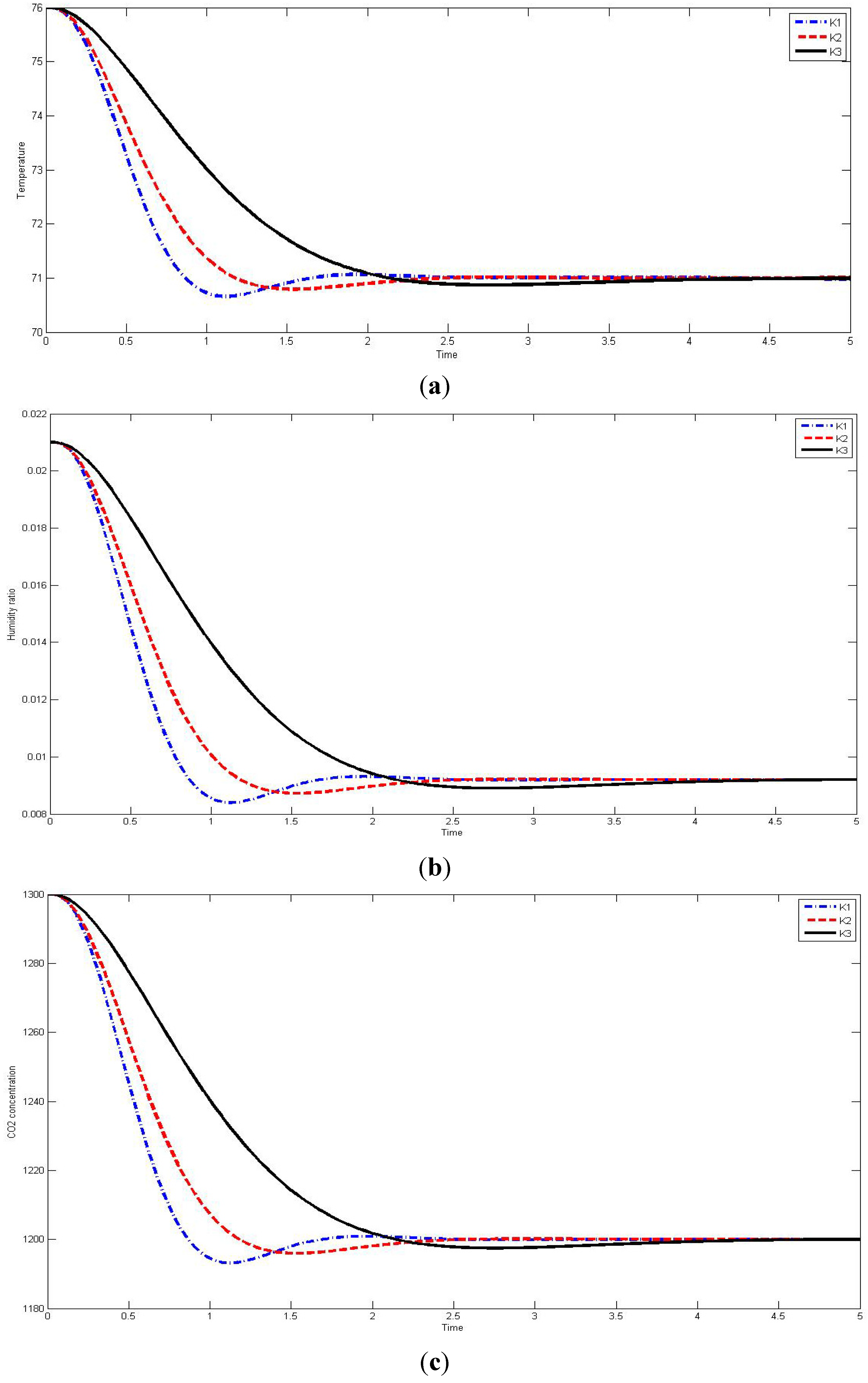
The gain K₁ corresponds to the case in which the pole is located at −2, −2, and −4, whereas the gain K₂ corresponds to the case in which the pole is located at −2, −3, and −5, and the gain K₃ corresponds to the case in which the pole is located at −5, −6, and −7. According to the pole placement, the control performance is varied. Figure 4 show the system responses in terms of temperature, humidity ratio, and CO₂ concentration, respectively. Table 3 shows the control performance metrics of settling time, rising time, settling max value, and settling min value for each value of gain.

Table 3. Control performance metrics of the pole placement controller.

	Temperature			Humidity ratio			CO2 concentration
	K1	K2	K3	K1	K2	K3	K1	K2	K3
Ts	3.2695	2.8431	1.1618	3.3889	2.7312	1.1595	3.3857	2.7270	1.1581
Tr	1.8919	1.5184	0.6804	1.8971	1.5124	0.6795	1.8970	1.5119	0.6794
Settling min	70.9962	71.0172	70.9927	0.0092	0.0092	0.0092	1200.1	1200	1199.9
Settling max	71.4929	71.4741	71.4297	0.0104	0.0104	0.0102	1209.9	1210	1208.5

Table 3. Control performance metrics of the pole placement controller.

	Temperature			Humidity ratio			CO2 concentration
	K1	K2	K3	K1	K2	K3	K1	K2	K3
Ts	3.2695	2.8431	1.1618	3.3889	2.7312	1.1595	3.3857	2.7270	1.1581
Tr	1.8919	1.5184	0.6804	1.8971	1.5124	0.6795	1.8970	1.5119	0.6794
Settling min	70.9962	71.0172	70.9927	0.0092	0.0092	0.0092	1200.1	1200	1199.9
Settling max	71.4929	71.4741	71.4297	0.0104	0.0104	0.0102	1209.9	1210	1208.5

Figure 4. (a) Temperature response for each pole placement; (b) Humidity ratio response for each pole placement; (c) CO₂ concentration response for each pole placement.

Figure 4. (a) Temperature response for each pole placement; (b) Humidity ratio response for each pole placement; (c) CO₂ concentration response for each pole placement.

4.2. Design of Linear Quadratic Regulator for Linearized HVAC System

The linearized HVAC system of (11) can be controlled by a linear controller. A linear-quadratic regulator (LQR) aims at designing stable controller which can minimize the cost function $J$ represents the performance characteristic requirement as well as the controller input limitation [17]. The cost function is:

$$J=\frac{1}{2}{{\displaystyle \int }}_0^{\infty }\left[{x^{\prime }}^{T}Q{x}^{\prime }+{\eta }^{T}R\eta \right]dt$$

(12)

where $Q$ is a positive semi-definite weight matrix and $R$ is a positive definite weight matrix. The weighting matrices $Q$ and $R$ are chosen by the Bryson’s rule (refer to Appendix A5) [18].

The feedback control law that minimizes the values of cost is:

$$\eta =-k^{\prime }e+y_d^{\left(3\right)}$$

(13)

where $e=x^{\prime }-Y_d={\left[e_1{e}_1^{\left(1\right)}{e}_1^{\left(2\right)}{e}_2{e}_2^{\left(1\right)}{e}_2^{\left(2\right)}{e}_3{e}_3^{\left(1\right)}{e}_3^{\left(2\right)}\right]}^T$; $K^{\prime }$ is given by $K^{\prime }=R^{-1}{B}^{T}P$; and $P$ is found by solving the continuous time algebraic Riccati equation:

$$A^{T}P+PA-PB{R}^{-1}{B}^{T}P+Q=0$$

(14)

Table 4 shows the gain values resulting from the LQR process solving algebraic Riccati equation.

Table 4. LQR gain values.

9 × 9 Gain matrix
$k_1^{\prime }$	diag([100 44.7850 9.9785],[100 44.7850 9.9785],[100 44.7850 9.9785])
$k_2^{\prime }$	diag([(100 54.7214 14.4721)],[(100 54.7214 14.4721)],[(100 54.7214 14.4721)])
$k_3^{\prime }$	diag([(100 88.6706 34.3124)],[(100 88.6706 34.3124)],[(100 88.6706 34.3124)])

Table 4. LQR gain values.

9 × 9 Gain matrix
$k_1^{\prime }$	diag([100 44.7850 9.9785],[100 44.7850 9.9785],[100 44.7850 9.9785])
$k_2^{\prime }$	diag([(100 54.7214 14.4721)],[(100 54.7214 14.4721)],[(100 54.7214 14.4721)])
$k_3^{\prime }$	diag([(100 88.6706 34.3124)],[(100 88.6706 34.3124)],[(100 88.6706 34.3124)])

The LQR controller was applied to the proposed HVAC system model (11) and the simulation results are shown in Figure 5. The temperature response of the proposed HVAC system is shown in Figure 5(a), and its humidity ratio response and CO₂ concentration response are shown respectively in Figure 5(b,c).

From these simulation results, we can see that the proposed HVAC system is effective, and that linear controllers are suitable for application to the proposed HVAC system model. Table 5 shows the control performance metrics of settling time, rising time, settling max value, and settling min value for each value of gain.

Table 5. Control performance metrics of the LQR controller.

	Temperature			Humidity ratio			CO2 concentration
	K1	K2	K3	K1	K2	K3	K1	K2	K3
Ts	1.4886	2.0107	3.2315	1.4982	1.9880	3.2028	1.5049	1.9873	3.1964
Tr	0.5279	0.7187	1.3093	0.5277	0.7189	1.3098	0.5277	0.7189	1.3098
Settling min	70.6601	70.7922	70.8702	0.0084	0.0087	0.0089	1193.2	1196	1197.5
Settling max	71.4249	71.3586	71.4777	0.0102	0.0100	0.0103	1208.5	1207.2	1209.6

Table 5. Control performance metrics of the LQR controller.

	Temperature			Humidity ratio			CO2 concentration
	K1	K2	K3	K1	K2	K3	K1	K2	K3
Ts	1.4886	2.0107	3.2315	1.4982	1.9880	3.2028	1.5049	1.9873	3.1964
Tr	0.5279	0.7187	1.3093	0.5277	0.7189	1.3098	0.5277	0.7189	1.3098
Settling min	70.6601	70.7922	70.8702	0.0084	0.0087	0.0089	1193.2	1196	1197.5
Settling max	71.4249	71.3586	71.4777	0.0102	0.0100	0.0103	1208.5	1207.2	1209.6

Figure 5. (a) Temperature response by LQR; (b) Humidity ratio response by LQR; (c) CO₂ concentration response by LQR.

Figure 5. (a) Temperature response by LQR; (b) Humidity ratio response by LQR; (c) CO₂ concentration response by LQR.

5. Conclusions

Herein we have presented a novel HVAC system model that considers not only temperature and humidity ratio, but also CO₂ concentration as the quantitative indices of comfort in a room. In applying an input-output feedback linearization method to linearize the HVAC system, problems of singularity, no relative degree, and interacting controls were encountered and a dynamic extension algorithm was used to solve these problems. The key contribution of this report is the addition of a continuous CO₂ concentration state and corresponding valve dynamics to a conventional HVAC system to allow continuous control of CO₂ concentration. Two types of linear controllers, pole placement and LQR controllers, were able to regulate the linearized HVAC system at the desired set point. Simulation results validated the proposed HVAC model, demonstrating its effectiveness in maintaining comfortable conditions. In future work, we will conduct further study on developing disturbance observer based controllers or intelligent controllers using fuzzy logic or artificial neural networks for a HVAC system considering parameter uncertainty and disturbance effect.