System for Road Vehicle Energy Optimization Using Real Time Road and Traffic Information

Abstract

Nowadays, reducing the energy and fuel consumption of road vehicles is a key issue. Different strategies have been proposed. One of them is to promote Eco-driving behaviour among drivers. Most Eco-driving tips take into account only the road stretch where the vehicle is located. However, larger improvements could be achieved if information from subsequent stretches is used. The main objective of this work is to develop a system to warn the driver in real time of the optimal speed that should be maintained on every road segment in order to optimize the energy used and the fuel consumed while observing a time schedule. The system takes into account the road vertical profile, the fixed and variable speed limits and the traffic information retrieved using V2V and V2I communications. The system has been tested on real road sections with satisfactory results in fuel savings.

1. Introduction

The current trend towards increased mobility in the most advanced societies runs counter to the criteria for controlling the greenhouse effect, local pollution and the exploitation of fuel resources. Increases in mobility and population becoming motorized represent also an increase in the demand for primary energy, and if fossil energy is used, it will mean a major increase in local emissions (nitrogen oxides NO_x, carbon monoxide CO, unburnt hydrocarbons HC and particles matter PM) and in the corresponding greenhouse gases emissions, so fuel consumption is an important issue in present-day society and there is intensive research into this issue. Reduction of fossil fuel consumption contributes to decreasing transportation costs and exhaust gas contaminants. In vehicles, energy and fuel consumption minimization is a complex problem because the power-train has different topologies and it is made up of several devices with many specific design features. In addition to power-train, the vehicle aerodynamics, other resistances and the influence of road vertical profile on fuel consumption must also be considered. To perform the energy minimization, general optimization techniques can be studied to analyse their computational load, the kind of minimum obtained and their feasibility to produce a response that represents the vehicle’s behaviour. Furthermore, driver manoeuvres can directly affect energy requirements. For this reason, informing the driver about the optimal speed to travel on a given road could reduce the fuel mass required to finish the current trip. This speed profile can be used to either feed an automatic system or to give advice to the driver.

2. Background

Efforts to reduce fuel consumption in automobiles, such as redesigning the internal combustion engine, reducing the mass and aerodynamic and rolling resistances [1] and using other propulsion technologies [2,3,4] have all been made. Today, optimization is present in the redesign of vehicle control systems [5] and other automotive parts [6] in order to obtain lower fuel consumption rates. There are several techniques utilized to optimize automobile power-train systems, such as, genetic algorithms (GA) [7], Simulated Annealing SA [8], Sequential Quadratic Programming (SQP) [9] and Dynamic Programming (DP) [10,11,12]. Several management strategies have been implemented for power-train control. These methods try to reduce the required energy. For example, different approaches tried to optimize hybrid vehicles operation. According to [13], global optimization is used when the optimization process uses a Hamilton-Jacobi-Bellman approach, such as DP. The results provided by DP can be considered as a benchmark for optimization [14,15] because it finds the global minimum value. The methods based on Calculus of Variations obtain a local optimization result, for example, Pontryagin’s minimum principle. Other examples of optimization can be found in [16,17,18,19].

In addition, other strategies have also been implemented. One of them is called Eco-driving. Eco-Driving can be described as the driving style followed by vehicle drivers to save fuel. This way of driving is based mainly on advance warnings and prediction, so the optimal average speed is selected at every instant and aggressive accelerations and decelerations are avoided by using traffic information and the geometric characteristics of the road ahead [20]. Classical Eco-driving tips have been widely distributed by car manufacturing companies, and some on-board devices can even collect data to monitor and evaluate the driving style. Eco-driving provides fuel savings from 15% [21] up to 25% [22]. In [23], the effect of driving style on fuel consumption and exhaust emissions is studied with the conclusion being reached that eco-driving can lead to 14% fuel savings but aggressive style increases consumption by 40%. Other authors present less positive figures, such as [24] with fuel savings of 3%–4%.

Eco-driving strategies can be learnt by drivers following certain rules. However, observance of those rules is quite subjective, because it is difficult to establish specific limits. Some tests have been carried out to determine the influence of average speed on fuel consumption and travel time. In [25], two different roads were driven along using the same Eco-driving style. Three different average speeds were obtained. The travel duration time and fuel consumption were measured. The results show fuel reductions of around 27.6%, 10.8% and 10.9% when the travel times were increased by 7.8%, 6.25% and 7.5% respectively. The proportion of fuel consumption savings and extra time were 3.52, 1.73 and 1.46. It can be observed from these results that fuel savings and extra time do not vary in the same way. They depend on factors such as travel distance, maximum allowed speed and the digital map of the road.

There are devices that show the driver the necessary instantaneous speed to arrive just-in-time at the destination [26]. These devices follow a reference travel time but fuel consumption is not considered. The driving style classification in [27] proved that, sometimes, on a given road, the total travel emissions using a low speed are higher than the total emissions when a higher average speed is used.

Other more complex systems can minimize fuel consumption without modifying the travel duration time [28]. In [24], fuel savings percentages of around 3%–4% are mentioned. In [29], experimental tests have demonstrated that a truck can reach a fuel reduction of 3.5% without modifying its travel duration time over a road distance of 120 km.

In automatic train control systems, similar concepts have been applied for optimize energy. Different approaches have been used such as analytical solutions [30,31] and nonlinear programming [32,33]. One of the main limitations of Eco-driving rules is the fact that they are based on the road stretches that the driver sees or on their previous knowledge of the route, but a positioning on a digital map could enhance the possibilities of making the right decisions in advance [34]. A more accurate and complete knowledge of the road geometry and precise advice on what to do at every instant could improve fuel savings by modifying driving styles. To overcome this limitation, [35] propose an algorithm that obtains the speed profile that provides the minimum fuel consumption to drive along a given road including the time as an additional variable within the optimization process. The problem of that approach appears in the fact that modifications in the event of unexpected situations cannot be done in real time due to the high computational time. Therefore, a new algorithm, that calculates the speed profile and optimizes fuel consumption while respecting a time schedule, is defined in [36]. This solution is based on approximate action rules defined from a DP algorithm, but results show that significant differences with the optimal solution can appear. Finally, anticipating variable conditions would improve results significantly as previous works have shown. For example, [37] show simulations with the effect of providing the driver with real time information on traffic and road conditions using vehicle-to-vehicle (V2V) and vehicle-to-infrastructure (V2I) communications.

3. Main Objective and Research Method

The main objective of this work is to develop a system to warn the driver in real time of the optimal speed that should be maintained on every road segment in order to optimize the energy used and the fuel consumed while observing a time schedule. The system takes into account:

-

Orography contained in a detailed digital map that includes the vertical profile with slope values

-

Speed limits, both fixed (signals contained in the digital map) and variable (because of weather conditions that can be transmitted to the vehicle in real time before the vehicle reaches that road section using V2V and V2I communications)

-

Information about traffic congestion that occurs periodically

-

Deviations from the optimal profile because of unexpected congestion (that can also be transmitted using communications) and, in general, when the driver does not follow the system speed suggestions

In this paper, given the initial hypothesis that there is a specific speed profile whose fuel consumption is the minimum necessary amount for reaching the destination within a previously established time, the solution proposed here is to create this speed profile by concatenating vehicle speed transitions as required. This chain-form solution is found by applying Dynamic Programming (DP) optimization. Taking account of the road vertical profile, allowed speed limits and timing relevance, DP chooses each constitutive part of the solution from a speed transitions set. Data for fuel consumption and duration time are associated with each speed transition. These associated data are obtained using an energy and fuel consumption model for longitudinal dynamic simulation.

Figure 1 shows the whole process scheme. In the optimization process, a driving state of a vehicle is described using the current speed and the gear engaged, and speed transitions can bring the vehicle from one state to another. When the state changes have been established, a model for energy and fuel consumption calculation provides the spent fuel and elapsed time for each transition. The fuel consumption model takes into account the road slope in each state change. When a transition (also called “atomic case”) has been simulated, values for initial speed, initial gear, final speed, final gear, spent fuel, elapsed time and road slope are stored into a look-up table. From now on, this look-up table containing the whole set of simulated transitions and their associated data is called fuel consumption map.

Then DP optimization technique is applied to find the optimal chain-form solution, i.e., the optimal speed profile. The optimal speed profile is created using an objective function to evaluate the speed transitions. The objective function considers spent fuel and elapsed time and contains weighting factors to assign different relevance to spent fuel and elapsed time. The optimal speed profile must satisfy the legal speed limits, with any speed transitions that exceed legal speed limits being excluded from the optimization process, and must consider the road vertical profile using the mathematical vehicle model. The weighting factor values are determined in order to meet a time schedule and to satisfy the destination arrival time.

Because the computational time of the DP algorithm is quite high when considering long distances, we have proceeded to divide the trip into shorter sections that are chained by overlapping stretches that allow an optimal solution by linking one to the next. Then, the DP algorithm is executed at the beginning of each overlapping distance for that specific stretch instead of the whole trip.

This strategy also allows the weighting factors to be modified if deviations between the optimal speed profile and the actual speed are found, in order to meet the schedule. This adjustment is made regardless of the vertical road profile and takes into account constant speeds between the road sections that have some type of restriction (fixed or variable limits, traffic congestion, etc.). A simplified DP algorithm is used for the whole trip, the factors that ensure reaching the destination on time are found, and are then applied to the next overlap in the complete DP algorithm. The simplified DP algorithm is based on the idea of only generating new alternatives when the speed limit changes for any reason, so the effect of the curve of dimensionality is not severe and execution time is reduced. Thus, during the trip, using V2V or V2I communications, the vehicle may receive information about any changes of speed limits or congestion in certain downstream road stretches, and optimal speed profile recalculation can be made in real time, firstly without considering road slopes to obtain the weighting factors and, secondly considering that road vertical profile and every speed limit type.

Figure 1. Scheme of the optimization process.

Figure 1. Scheme of the optimization process.

4. Algorithm for Energy and Fuel Consumption Minimization

The performance maps of the multiple power-train devices, the high nonlinear behaviour of these devices and their discontinuities are typical challenges presented in fuel consumption modelling. According to [38], these characteristics make the system hard to model without including simplifications. Ruled-based controllers, e.g., fuzzy controller, find non-global minimums and do not match detailed vehicle behaviour but they have an easy implementation [39]. DP warranties a global minimum. Also, it can handle nonlinear non-convex problems and it does not need to be tuned according to drive-train topology [19]. For these reasons, DP is chosen as the optimization strategy to obtain the speed profile that reaches the minimum fuel consumption.

4.1. Dynamic Programming (DP)

DP is an optimization method that minimizes an objective function by evaluating all possible control sequences. Every state transition of the system involves a cost. The optimal control sequence is built by joining the specific state’s sequence that obtains the least total cost. The cost of each state transition is defined by an objective function. Although DP needs a long computational time, it finds the global minimum in an optimization process.

Bellman’s Principle of Optimality [40,41] is the theoretical support for Dynamic Programming. This principle states that all the portions of an optimal trajectory are, by themselves, optimal trajectories [42]; i.e., for a given state, the optimal rule for the following transitions does not depend on the rule applied in the previous transitions.

In [43], a typical optimization problem is solved by using DP. The requirement is to find the input sequence or optimal decision sequence that minimizes the following objective function:

$$J={\displaystyle {\sum }_{k=0}^N{q}_k(x(k),u(k))}$$

(1)

where, x is the state variable; u is the decision variable; and k is the stage.

This cost value depends on the initial time i, the initial state x(i) and the input variable u in the interval [i, N], but the cost does not depend on any previous states. For the trajectories that in instant i are in state x(i), the optimal cost depends only on the initial state x(i) and the initial time i:

$$J_i^{*}=\underset{u}{\min }\left\{{\displaystyle {\sum }_{k=i}^N{q}_k[x(k),u(k)]}\right\}=J_i^{*}[x(i)]$$

(2)

Then, Bellman’s Principle of Optimality indicates that:

$$J_i^{*}=\underset{u(i)}{\min }\{q_i[x(i),u(i)]+J_{i+1}^{*}[x(i+1)]\}$$

(3)

Additionally, x(i + 1) depends only on x(i) and u(i). Therefore, when we minimize with respect to u(i), the optimal cost in i will depend only on x(i) and i. So, using iterative application of Equation (3) and collecting the results from the final state back to the initial state (backward recursion), the optimal input sequence u can be found. The aforementioned problem can be solved using either backward or forward recursion. The results obtained by both methods should be the same.

4.2. Optimization Data Set

Our proposed approach for fuel consumption optimization is a chain-form solution generated by DP technique. The implemented DP algorithm concatenates speed transitions to form the optimal speed profile that minimizes fuel consumption. Speed transitions can describe changes on vehicle behaviour if the driving states are defined using the vehicle speed and the gear engaged. In this way, the speed transitions can represent acceleration, deceleration or a constant speed stage. The acceleration and deceleration curves of the vehicles can be defined in different ways [44,45]. For simplicity, constant acceleration, depending on the gear engaged, is considered for speed transitions of the vehicle, according to [39].

In the speed transitions, speed and distance are discretized. Speed discretization is performed according to the desired resolution of the optimal speed profile. The distance Dg indicates the speed transition length. Dg can be made up of one or more minimum discrete steps of distance. In acceleration and deceleration cases, the gears have a different assigned distance Dg because high gears need a longer distance to change the car speed among discrete speed values than low ones. In the constant speed cases, the minimum discrete step for distance is assigned whichever gear is used in the speed transition because the speed does not change.

The DP algorithm evaluates the speed transition to find the optimal speed profile, therefore the speed transition must be tagged with a quantitative feature. In this method, the speed transitions are tagged using their spent fuel and elapsed time. A fuel consumption model must be used to estimate these variables. The numerical data of initial speed, final speed, initial gear, final gear, simulated road slope, spent fuel and elapsed time for each speed transition are stored into a look-up table. This data set describing the associated features of an individual speed transition is called “atomic case”. Each atomic case is an entry for the look-up table. This look-up table feeds to the DP algorithm and contains the necessary data to perform the optimization process.

In the DP algorithm, two sequences only can be compared if the following conditions are fulfilled: they have the same initial and final speed and the same initial and final gear, and they are limited by the same distance points. When two or more sequences of states are compared, only the sequence with the lowest cost is preserved. DP takes into account the road vertical profile and legal and safe speed limits contained in a digital map when it concatenates the necessary atomic cases to find the optimal speed profile.

4.3. Fuel Consumption Model

To generate the previous look-up table, a mathematical vehicle model is used. Depending on the dynamics and detail level of the simulated variables, the models can be classified into quasi-static models and dynamic models. Energy, consumption, performance and emissions studies can be simulated by means of quasi-static models [46,47,48]. A quasi-static fuel consumption modelling can follow either a forward-looking or a backward-facing approach. The backward-facing approach assumes the vehicle exactly describes a speed profile to calculate the fuel consumption [49]. The forward-looking approach needs a driver model to follow the target duty cycle [50]. This driver model is usually implemented as a PID controller to generate acceleration and brake commands [51,52].

Quasi-static models have a shorter simulation time than dynamic models but their exactitude is lower. Simulation differences between these two kinds of models are smaller than 5% and the simulation time proportion is close to two orders of magnitude [53]. The quasi-static models include fuel consumption and power train efficiency as static maps by means of look-up tables [46,54].

Examples of quasi-static vehicle simulators are QSS-Toolbox [55,56] and ADVISOR [57,58]. In contrast, PSAT [59], CARSIM [60,61] and V-ELPH [62] use dynamic models to perform their simulations.

In this paper, a quasi-static vehicle model was chosen because it provides a low computational time and, according to [63], its accuracy varies approximately around 4% from fuel mass estimations based on dynamic methods.

Our energy and fuel consumption model takes the mathematical methodology from QSS-Toolbox [55] but the implementation is different. QSS-Toolbox contains the equations necessary to perform a longitudinal dynamics simulation [64] and calculates the fuel consumption for a determined duty cycle and provides fuel consumption, accelerations, car speed, aerodynamic forces, and other variables versus time. Contrary to QSS-Toolbox, our fuel consumption model accepts as input a speed cycle that varies in the distance domain. Fuel consumption expressed as a function of distance is a requirement because the optimization process takes into account the legal and safe speed constraints and these limits are defined in the space domain. The model implementation allows a flexible scheme to vary input parameters of the simulation such as initial speed, final speed, slope, gear and simulated distance. This flexibility is useful when spent fuel and elapsed time calculation is performed for each speed transition.

Table 1 shows the main model parameters. Furthermore, the fuel consumption model contains global operational limits for vehicle operation, e.g., maximum engine torque and minimal speed according to the gear engaged. Other more specific limits can be adjusted such as the maximum engine speed and user-defined acceleration/deceleration ranges. Vehicle parameters can be configured, so atomic cases contained in the look-up table depend on the vehicle type and they are calculated once at the beginning of the algorithm execution.

Table 1. Main vehicle model parameters.

Vehicle	Transmission	Engine
Mass	Number of gears	Fuel
Rotating mass	Gear ratios	Engine displacement
Frontal area	Differential ratio	Engine inertia
Drag coefficient	Gearbox efficiency	Torque-speed curve
Rolling friction coefficient	-	Engine speed at idle
Wheel radius	-	Power required by auxiliaries
-	-	Engine torque at fuel cutoff

Table 1. Main vehicle model parameters.

Vehicle	Transmission	Engine
Mass	Number of gears	Fuel
Rotating mass	Gear ratios	Engine displacement
Frontal area	Differential ratio	Engine inertia
Drag coefficient	Gearbox efficiency	Torque-speed curve
Rolling friction coefficient	-	Engine speed at idle
Wheel radius	-	Power required by auxiliaries
-	-	Engine torque at fuel cutoff

4.4. Objective Function

According to DP theory, the sequences of transitions must be assessed using an objective function. Every speed transition has travel time and fuel consumption figures. Fuel mass and time can be used to compute the sequence assessment. This assessment could be defined as an operational cost such as [65] do. In [65], the operational costs are divided into monetary factors per fuel quantity and time units. A similar approach is made by [66,67] where the evaluation is realized by the arithmetic sum of the spent fuel and travel time. The travel time importance is modulated using weighting factors. Following this line, the chosen objective function (8) joins the fuel consumption and travel time into a single cost for every transition. Weighting factors are included in the expression to assign different relevance to the fuel consumption mass and the travel time:

J = α (fuel consumption) + β (travel time)

(4)

Weighting factors α and β are non-negative real values, excluding the case of both zeros and they are calculated during the vehicle trip as following sections explain. Fuel consumption is expressed in milligrams and the time in milliseconds.

4.5. Slope Influence over Atomic Cases Selections

In our optimization approach, the optimal solution is a sequence of states (speed, gear) as a function of distance. Considering that state transitions have different costs depending on the road slope, so, in the look-up table, there are various entries with the same transition but different cost; each entry represents a different slope condition.

When our algorithm finds a situation in which a state transition is carried out over a road section with several slope values, an average slope value is calculated to assign the cost for this state transition. When the algorithm finds that one of the slope values of a multi-slope road section cannot be run using a gear number, the algorithm chooses another sequence with a different gear number to be used for that determined slope value. This is the typical scenario in which a driver must shift to a lower gear when the current gear number is not able to raise the speed during a road section with positive slope.

4.6. Overlap of DP Solutions of Road Stretches

Depending on the variables considered in the dynamic programming and its discretization, the execution time of the algorithm can be very high. This is due to the exponential increase in the number of possible solutions created in each iteration. The basic optimization algorithm presented in [35] takes 49 seconds to find the speed profile of a trip of only 20 km, but this runtime increases linearly if a longer route is considered for fuel consumption optimization. Therefore, new ways must be found to achieve results that can be evaluated in real time or at least give the driver tips for optimal speed on each section with a low significant delay.

In [66] simulations are performed of how long the road stretch taken into account should be in the dynamic programming strategy and indicated that fuel consumption savings tend to be constant with distances of over 2 km.

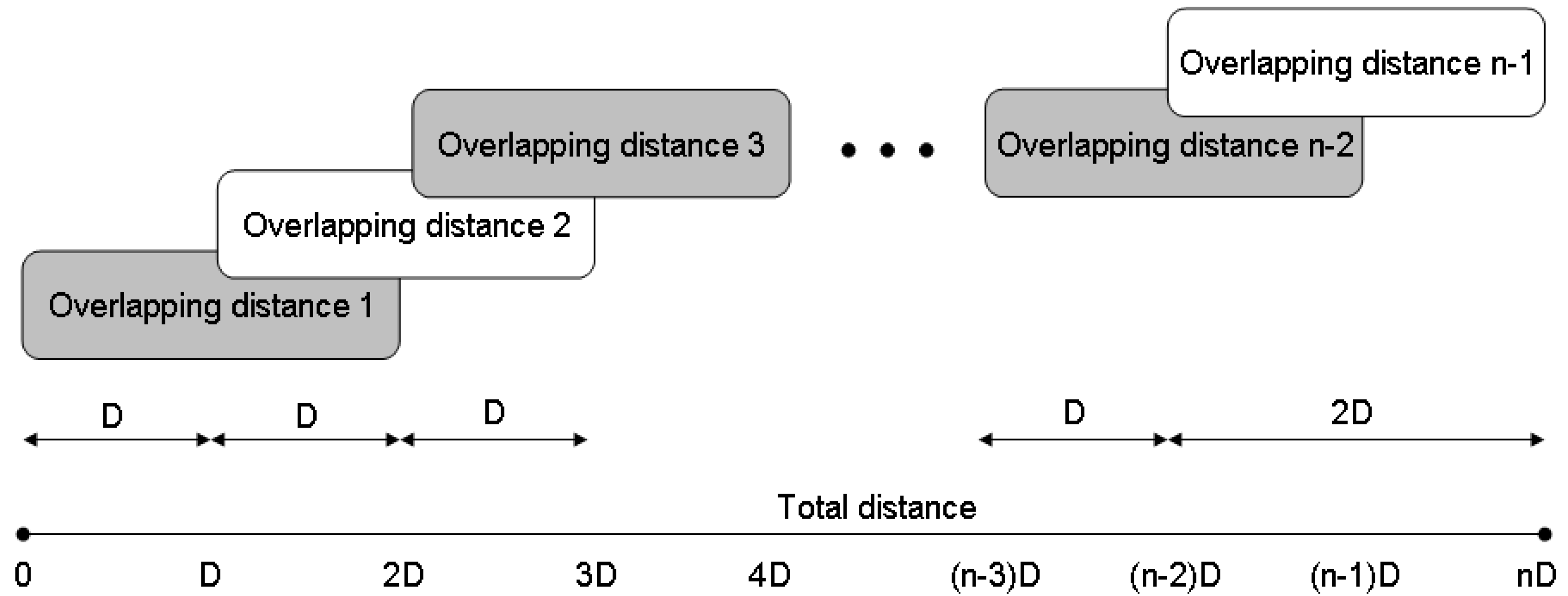
Considering this fact, an evolution of the DP algorithm is presented, consisting in overlapping two partial speed profiles. If the length of these sections and the overlaps are long enough, it is found that the speed profile created by overlapping partial optimal speed profiles closely resembles the profile of the entire trip. Figure 2 explains the method used.

With D being the length of the partial speed profiles and nD the total trip length, an optimal speed profile is calculated for the road stretch between 0 and 2D starting with the vehicle speed at the point of distance 0 and ending with a zero speed at the point of distance 2D. This profile is used as a solution for the stretch between 0 and D, setting the speed at point D as the initial speed for the following DP algorithm execution. From point D, the second partial speed profile is obtained in a new DP algorithm run that finishes at point 3D. In this case, a valid solution is taken between D and 2D, and so on. The union of all partial speed profiles calculated provides the approximate optimal speed profile for the whole trip.

The final selection of D depends on two factors: (1) differences between approximate solution and optimal one should be small; (2) the overlapping distance should not be very long because optimal speed updates considering real driving conditions are performed every D stretches and those updates should be quite frequent. Tests have been made varying overlapping distances for a trip of 20 km, and the results are shown in Table 2. Therefore, we have chosen overlap stretches of 5 km, longer than the 2 km stretches proposed in [66], because this value provides a short computational time and results accuracy is significantly improved.

Figure 2. Overlap of the partial speed profiles.

Figure 2. Overlap of the partial speed profiles.

Table 2. Differences between the optimal speed profile and the approximate speed profile using overlaps.

Overlap Distance (km)	Fuel Consumption Difference (%)	Travel Time Difference (%)
1	−3.73	8.27
2	−0.50	0.40
3	0	0.17
4	0.04	−0.07
5	0	0.01

Table 2. Differences between the optimal speed profile and the approximate speed profile using overlaps.

Overlap Distance (km)	Fuel Consumption Difference (%)	Travel Time Difference (%)
1	−3.73	8.27
2	−0.50	0.40
3	0	0.17
4	0.04	−0.07
5	0	0.01

This process makes the DP algorithm be performed every D meters, so it is possible to adjust the weighting factors in each run to ensure that the destination is reached on time taking into account the deviations from the optimal speed profile and modifications in speed limits or the appearance of unforeseen traffic congestion situations.

4.7. Weighting Factors Calculation

Because the driver may voluntary cease to follow the optimal speed profile or a traffic jam may force him to do so, a new speed profile should be calculated to meet the desired travel time. The computing time of the new profile should be short enough for the user of the system not to perceive a prolonged interruption of information on the proper speed.

The idea is to provide the algorithm with the necessary tools so that the maximum travel time is met after suffering the delay caused by the traffic jam. To accomplish this, the strategy used by the optimization system is based on the input of the average speeds of every road section, depending on the time of day. To recover the time lost during the trip, the average speed is modulated based on the remaining travel time. This speed modulation is accomplished by adjusting the weighting factor β of Equation (4) in each distance overlap. Specifically, the influence of α/β parameter on consumption and travel time is shown in [35]. It should be noted that there is an interval in which these parameters are influenced by the α/β ratio, but, out of this interval, the influence of this ratio is negligible. Thus, optimization at the beginning of each overlap distance is performed in two steps:

• DP algorithm for the entire remaining distance to the destination without considering the slopes and allowing only changes in the speed on those road sections where there is a speed limit change (fixed, variable or because of traffic). This algorithm looks for the concatenation of constant speed stretches that provide minimum fuel consumption but allows the vehicle to reach the destination on time.
• For the actual overlap stretch, the correspondence between the resulting speed of the previous step and a new value of β is found. This value is used in the DP algorithm for the stretch considering the vertical road profile. This second run of the DP algorithm provides the speed profile of which the driver is informed.

It should be noted that the computational time of the first step is reduced because expansions of DP solutions are produced only on a limited number of road sections.

4.8. Influence of Traffic Conditions

There are systems like the one presented in [30] that take into account the speed limits and recommend the driver the speed in order to reach the destination on time. One characteristic that the proposed system includes is the recalculation process of the optimal speed profile considering the traffic conditions. Data from the traffic conditions are considered according to the following two situations:

-

Traffic jams that appear periodically, so they are well-known and predictable and can be considered as stretches with a variable speed limit.

-

Unforeseen traffic jams that are transmitted to the vehicle via V2V or V2I communications.

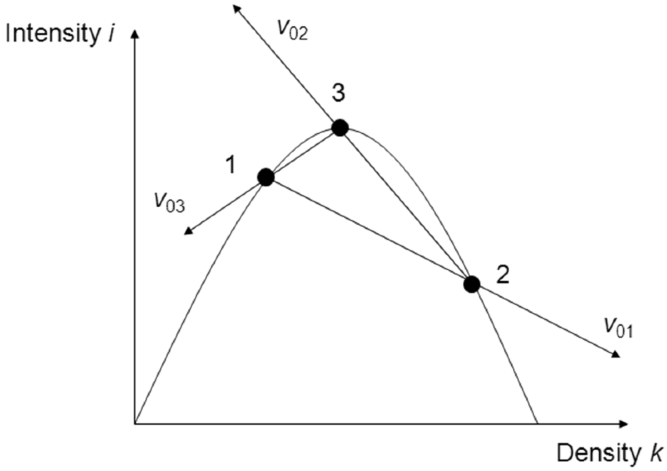
In the second case, the traffic jam progression is not known a priori. For this reason, the system uses the Greenhields linear traffic model [68,69]. Hence, as Figure 3 shows, initial traffic conditions are denoted by point 1 (speed v₁, density k₁, intensity i₁) and traffic perturbation forces to move to point 2 (v₂, k₂, i₂). When the perturbation disappears, the traffic state point moves to the maximum intensity conditions 3 (v₃, k₃, i₃) and then the initial conditions are recovered.

Figure 3. Operation traffic states when a perturbation appears.

Figure 3. Operation traffic states when a perturbation appears.

According to the traffic shock waves theory, the perturbation will propagate downstream at a speed of v₂ and upstream at a speed of:

$$v_{01}=\frac{i_1-i_2}{k_1-k_2}$$

(5)

so traffic between both waves is characterized by condition 2.

When the perturbation disappears, a new shock wave appears at the head of the traffic jam that propagates upstream at a speed of:

$$v_{02}=\frac{i_2-i_3}{k_2-k_3}$$

(6)

So traffic between the sections defined by the head of the jam and that wave will have the characteristics defined by state 3.

Finally, when the second shock wave reaches the first one, the initial conditions 1 will be recovered by means of a new wave that moves downstream from the tail of the traffic jam at a speed of:

$$v_{03}=\frac{i_3-i_1}{k_3-k_1}$$

(7)

Hence, from the knowledge of the initial traffic conditions 1 and the properties of the perturbation (state 2), it is possible to evaluate the traffic jam evolution and obtain the maximum length L of the traffic jam and the time T that initial conditions take to be reset.

$$L=v_2\cdot T_p-v_{01}\cdot \left(\frac{\left(v_2-v_{01}\right)\cdot T_p}{v_{01}-v_{02}}+T_p\right)$$

(8)

$$T=T_p+\frac{\left(v_2-v_{01}\right)\cdot T_p}{v_{01}-v_{02}}+\frac{v_2\cdot T_p-v_{01}\cdot \left(\frac{\left(v_2-v_{01}\right)\cdot T_p}{v_{01}-v_{02}}+T_p\right)}{v_{03}}$$

(9)

where T_p is the perturbation duration.

5. Results on a Real Road Section

The optimization algorithm was applied to a long distance trip of approximately 100 km on the route between Madrid and Barcelona (Spain) along the A2 highway. The road geometry was measured using an instrumented vehicle with an Astech G12 GPS receiver (Thales Navigation, Inc. Santa Clara, CA, USA) and an inertial measurement system comprising a Correvit L-CE- non-contact speed sensor (Corrsys-Datron Sensorsysteme GmbH. Wetzlar, Germany) and an RMS FES 33 gyroscopic platform (RMS Dipl.-Ing Schäfer GmbH & Co, KG. 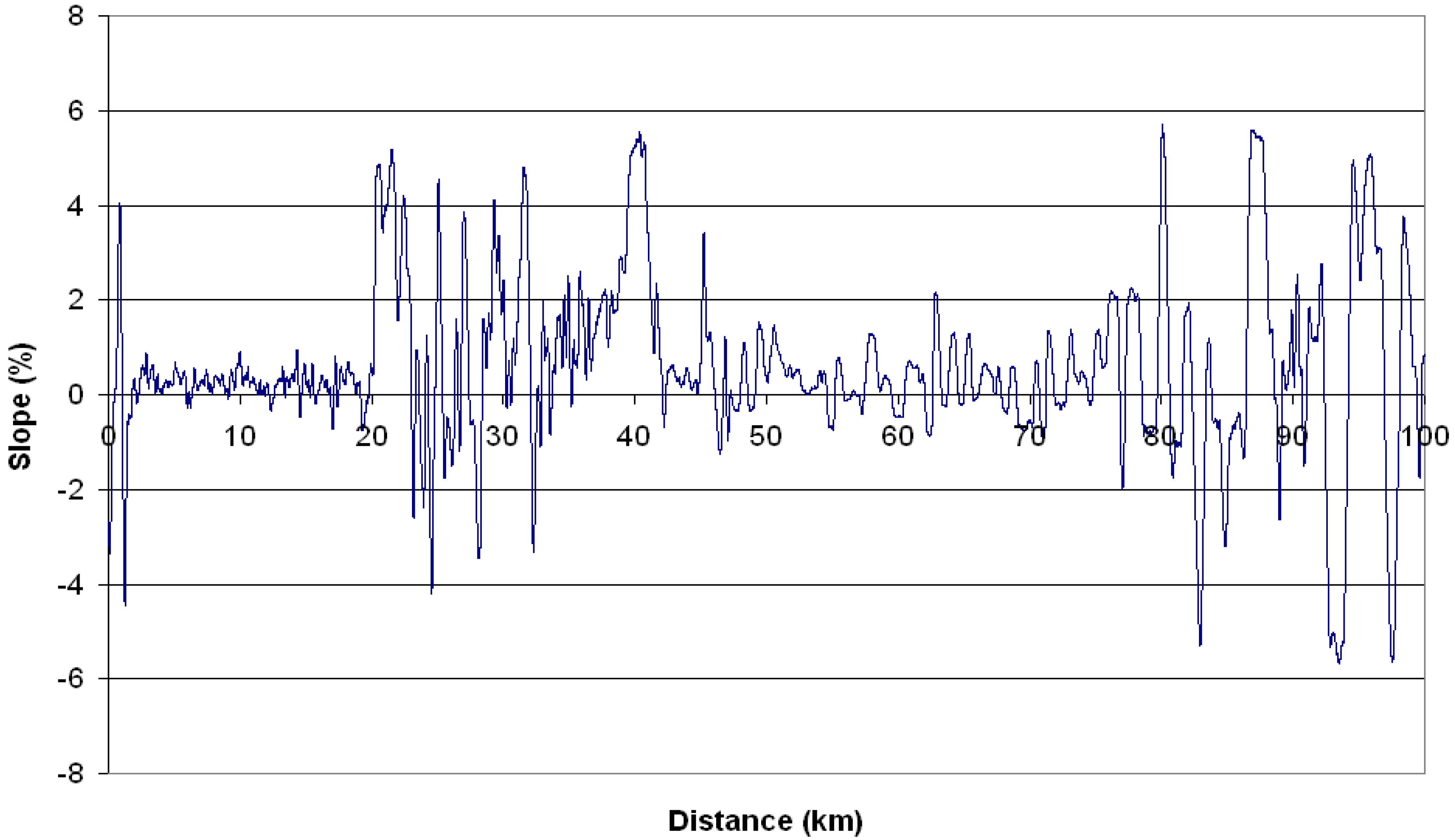Hamburg, Germany) [70,71,72,73]. The slopes profile is shown in Figure 4. Additionally, fixed and variable speed limits have been identified (Table 3). The vehicle is a Ford Focus with a ZETEC 2 litre petrol engine (Ford Motor Company. Dearborn, MI, USA).

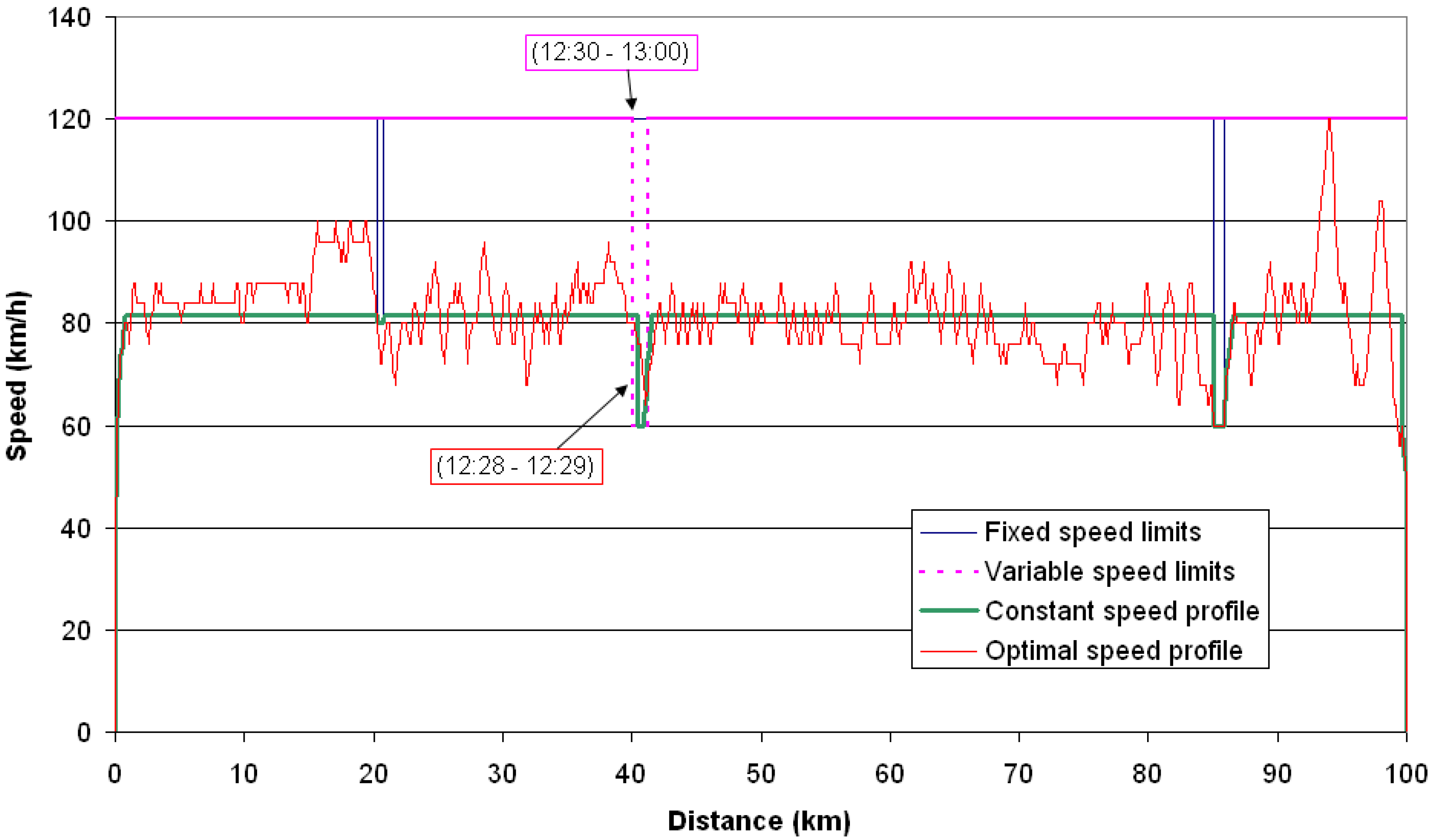
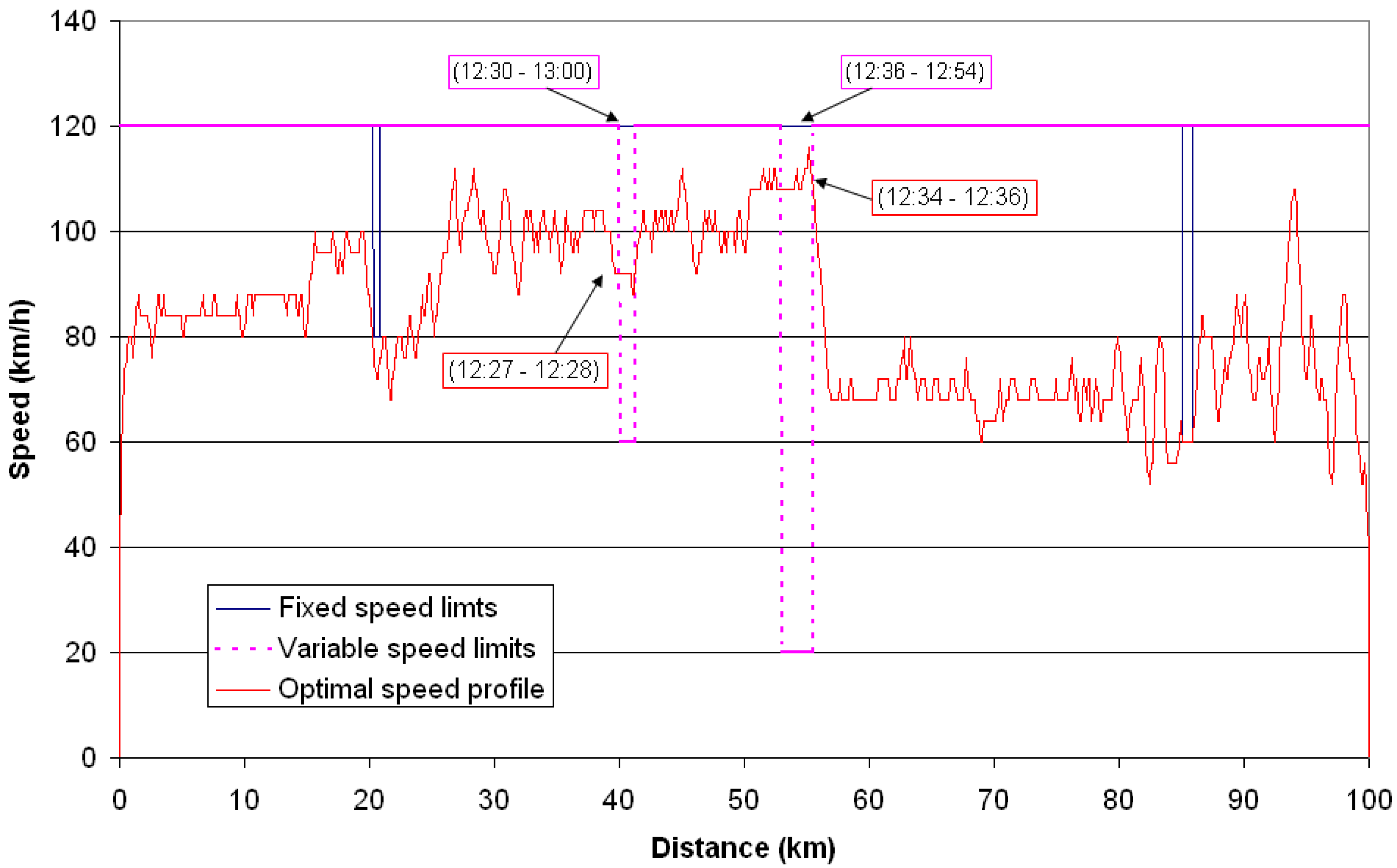
It is considered that the trip begins at 12 h and the arrival time is expected at 13:15. The system defines the optimal speed profile (Figure 5) considering the speed limits and informs the driver. Comparing this speed profile with a constant speed one that provides the same travel time, except stretches with some kind of limit, fuel savings of 4.0% have been obtained, assuming that the acceleration and deceleration processes are similar in both cases. This fuel savings value is similar to that presented in [35], but a little bit lower because large trip distances with flat vertical profiles diminish the optimization effect. The system takes advantage of the knowledge of the variable speed limits in order to find the best strategy in which the effect of those kinds of limits is reduced, adapting the speed before and after them and fuel savings remains in significant values. In this sense, the system could recommend speeding up (as can be seen in Figure 6) or slowing down to reduce the amount of time the vehicle is involved in the traffic limit section when the limit is active.

Figure 4. Road slopes profile.

Figure 4. Road slopes profile.

Figure 5. Optimal speed profile (only fixed and variable speed limits expected before the trip begins).

Figure 5. Optimal speed profile (only fixed and variable speed limits expected before the trip begins).

Table 3. Speed limits (below the generic road speed limit of 120 km/h).

Stretch (km)	Speed Limit (km/h)	Limit Type	Limit Schedule
20.3–20.8	80	Fixed	0–24 h
39.8–41.0	60	Variable	12:30–13:00
85.1–85.9	60	Fixed	0–24 h

Table 3. Speed limits (below the generic road speed limit of 120 km/h).

Stretch (km)	Speed Limit (km/h)	Limit Type	Limit Schedule
20.3–20.8	80	Fixed	0–24 h
39.8–41.0	60	Variable	12:30–13:00
85.1–85.9	60	Fixed	0–24 h

Figure 6. Constant speed profile (unexpected speed restriction).

Figure 6. Constant speed profile (unexpected speed restriction).

Furthermore, the system can adapt in real time the information provided to the driver according to the new information that the vehicle receives along the trip by wireless communications between vehicles or with the infrastructure. The network access devices used are MTM-CM3100 (Maxfor Technology Inc. Seongnam, Korea), based on the TelosB platform (Memsic Inc. San Jose, CA, USA). This allows connectivity with any computer platform and acts as a gateway to access the vehicular GeoNetwork. This device works under Linux (TinyOS) operating system (an open source software). In order to access the wireless network to 2.4 GHz in mesh, it uses the IEEE 802.15.4 standard at physical and link level and a mesh routing protocol, which guarantees the desired functionality of the VANET at transmission rates up to 250 Kbps and in a range of 100 meters. 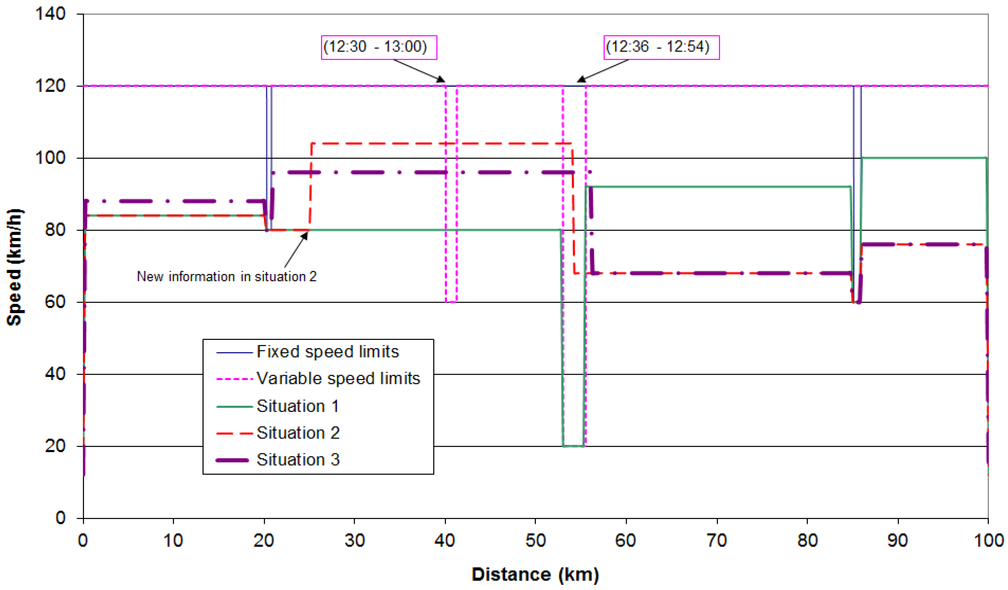That way, Figure 6 and Figure 7 show how the system adapts the speed profile when the vehicle receives the information about a traffic perturbation between kilometric points 53 and 55.5 that makes vehicles move at an average speed of 20 km/h between 12:36 and 12:54. Figure 6 presents the constant speed profiles between road sections with special speed limitations defined by step 1 of the method described in Section 4.7. in the following three situations:

• The system does not obtain any information about this traffic perturbation until the vehicle reaches the road section of kilometric point 50 (quite near to the perturbation section), so it maintains the same speed profile until the perturbation forces the vehicle to miss it.
• The system receives the information when the vehicle is located at kilometric point 25, so the speed profile is adapted from that point in order to meet the established schedule.
• The system receives the information at the beginning of the trip, so the speed profile is adapted from that point in order to meet the established schedule.

In the first situation, the system does not adapt the speed profile until the vehicle finds the speed restriction so no action is taken in advance to avoid it. As can be observed in case 2, as soon as the system receives information on the perturbation not considered at the beginning of the trip, the constant speed profile is recalculated in order to reach the destination on time and take advantage of the information so the speed is adapted so that this perturbation will have a minor effect on consumption. Then, using the β weighting parameter that corresponds to the constant speed of the current road overlap stretch, fuel optimization considering road slopes is performed. Hence, the vehicle adapts its speed before the driver can perceive the traffic congestion visually. In case 3, speed restriction is known from the beginning so the optimal speed profile can be calculated in advance in a similar way as previously shown.

Figure 7 shows the final optimal speed profile when the information is obtained in advance (at kilometric point 25). The fuel savings obtained between the three situations analysed reaches 3.8% (when comparing case 2 and case 1) and 3.9% (when comparing case 3 and case 1), but it should be noted that these results depend on the specific situation. This is because the anticipation of information delivery, traffic congestion characteristics, and the road stretch in which the perturbation happens, are key variables that limit or enhance the optimization possibilities. Finally, apart from energy savings, the distribution of information on unexpected events in advance improves the reliability of the system in meeting the time schedule because corrective actions can be taken before and, therefore, the adaptation of the speed profile provides better results.

Figure 7. Optimal speed profile (unexpected speed restriction).

Figure 7. Optimal speed profile (unexpected speed restriction).

6. Discussion

In this paper, the speed optimization problem has been solved using DP. This technique guarantees the global optimal solution even if the problem has non-convex constraints. This is the advantage over other approaches such as Genetic Algorithms, because these methods could have a high probability to get the global optimal solution [33], but it is not actually guaranteed. So there are optimization techniques that can work with non-differentiable equations and restrictions but they require approximations and some of them do not guarantee reaching global optimum but local ones.

The main drawback for DP is the exponential growth of calculation time caused by the number of inputs and states (curse of dimensionality). The calculation time increases with the length of the horizon and this fact makes onboard real-time optimization for a complete trip unfeasible when long distances are considered, so a stretch overlapping method has been used in order to shorten the road stretches length in which DP is performed. This method allows, on the one hand, real time execution that provides approximate solutions but very similar to the optimal ones. On the other hand, periodic modifications of weighting factors are made in the event that traffic conditions change or the driver has not followed the optimal speed profile. This approach provides an approximate solution but the overlapping distance has been chosen considering that differences between the approximate solution built concatenating stretches and the optimal one should be small. The selected distance D seems to be appropriate because these differences are quite reduced. Furthermore, the warning updates are frequent enough for counteracting any speed deviation during the trip.

Other methods apart from DP could be used and can be found in previous research, but the problem type, the complexity of the system analyzed and the accuracy required make that DP is an adequate approach providing a better behaviour that other mathematical tools. For example, in Lagrangian methods, the constraint functions could have to be approximated in order to obtain features for differentiation and convexity. An energy consumption optimization for road vehicles contains several data sets (one of the most complex ones could be the engine map) into look-up table forms and these data could be hard to be fitted by a function without doing approximations. The differences on the results when the model functions are replaced by approximations are discussed in [74]. Furthermore, in [75], the author comments some disadvantages when a vehicle energy optimization is done using nonlinear programming.

Regarding the system operation, it should be noted that the system does not provide any warnings when a traffic congestion situation is detected, because the driver could not follow them and he must adapt his speed to the traffic conditions. But the system recalculates the speed profile for completing the trip in the predefined travel time when these traffic conditions disappear. In general, under complex scenarios, the driver is not forced to follow the system indications so it will compensate any deviation afterwards.

Another relevant topic that should be highlighted is the fact that the system, apart from traffic conditions and legal speed limits, considers other types of speed limits, such as safe speed limits that can differ from legal speed limits under certain circumstances (vehicle type, adverse weather conditions, etc.). These safe speeds are calculated according to the method described in [76,77] and they are stored in the digital map. Then, if variable conditions are detected during the trip and retrieved by wireless communications, speed limits can be updated and the algorithm recalculates the optimal speed profile according to these new limits.

Finally, the fuel minimization system has been applied on a real highway section and fuel savings of up to 4% were obtained with respect to a constant speed profile with the same travel time. Our optimization strategy obtains fuel savings lower than those given for strategies such as [25,26] that do not include the travel time in the fuel minimization process, but optimal speed profiles produced by our DP algorithm produce slightly higher fuel savings than other similar systems [28,66] that involve travel time within the fuel consumption optimization process. Furthermore, the adaptation to unexpected traffic situations in real time, both when receiving information in advance or under sudden deviations, is another of the main advantages of the proposed algorithm that improves energy consumption savings. More specifically, and considering that these results highly depend on the characteristics of the traffic perturbation, fuel savings of 3.8% and 3.9% (depending of the road section where dynamic information is received) have been registered in relation to the situation without the wireless communication system.

The system has been implemented considering a human driver, but results are also valid when autonomous driving is used. The system estimates average acceleration and deceleration processes that could be different from the ones performed by a human driver depending on his driving style, so final fuel consumption and time could slightly differ from the theoretical ones. However, this fact is not significant for the whole trip when considering interurban roads. Furthermore, if human behaviour produces large time deviations, the algorithm is able to compensate them. In the case of urban environments, these speed transitions have a higher relevance and traffic lights state is crucial for optimizing fuel consumption. It should be noted that the same architecture would be valid in this case because communications between vehicles and the infrastructure could provide the necessary information but overlapping stretches length used in the algorithm execution should be reduced.

7. Conclusions

An optimization system based on Dynamic Programming theory has been implemented to perform energy and fuel consumption minimization in vehicles with a conventional power-train. The algorithm concatenates speed transitions to form the optimal speed profile that produces the minimal fuel consumption for a determined trip. This speed profile is provided to the driver in real time thanks to an ad-hoc interface. This algorithm uses a quasi-static model to obtain the energy and fuel consumption data. The speed sequences are evaluated using an objective function that takes into account fuel consumption and duration time for each speed transition. Weighting factors are included in this function in order to give different relevance to the fuel consumption and duration time during the optimization process and are used to guarantee that the time schedule of the trip is met. The road vertical profile is considered to carry out the fuel optimization. Maximum fixed and variable speed constraints are included within the optimal solution search.

This paper presents several improvements in relation to the fuel optimization algorithm based on Dynamic Programming implemented in [35]. Furthermore, the results are improved when comparing them with the approximate solution provided by the method presented in [36]. One of the most relevant improvements is the mechanism that guarantees, if possible, reaching the destination on time. This fact has been achieved taking into consideration speed limits and possible traffic jams, as well as information obtained through wireless V2V and V2I communications. With these data, the system knows periodic traffic jams and unexpected perturbations in advance, so it can calculate the average speed on each road stretch between two consecutive sections with speed limits. In a subsequent step, the system optimizes energy consumption considering the road vertical profile.