Valuation of Wind Energy Projects: A Real Options Approach


Abstract
: We address the valuation of an operating wind farm and the finite-lived option to invest in it under different reward/support schemes: a constant feed-in tariff, a premium on top of the electricity market price (either a fixed premium or a variable subsidy such as a renewable obligation certificate or ROC), and a transitory subsidy, among others. Futures contracts on electricity with ever longer maturities enable market-based valuations to be undertaken. The model considers up to three sources of uncertainty: the electricity price, the level of wind generation, and the certificate (ROC) price where appropriate. When analytical solutions are lacking, we resort to a trinomial lattice combined with Monte Carlo simulation; we also use a two-dimensional binomial lattice when uncertainty in the ROC price is considered. Our data set refers to the UK. The numerical results show the impact of several factors involved in the decision to invest: the subsidy per MWh generated, the initial lump-sum subsidy, the maturity of the investment option, and electricity price volatility. Different combinations of variables can help bring forward investments in wind generation. One-off policies, e.g., a transitory initial subsidy, seem to have a stronger effect than a fixed premium per MWh produced.1. Introduction
Smart grids in the EU are defined as “electricity networks that can intelligently integrate the behaviour and actions of all users connected to it—generators, consumers and those that do both—in order to efficiently deliver sustainable, economic and secure electricity supplies” [1]. Thus, the price of electricity is a major concern. As long as other concerns like the environmental impact of power generation come to the fore, the economic profitability of renewable energy facilities too becomes important. As a matter of fact, renewable energy sources (RES) are becoming ever more relevant in the generation of electricity (RES-e). Major drivers are the decreasing costs of renewable technologies and strong support from government agencies. This trend is expected to continue in the years ahead (European Commission [2]). Pérez-Arriaga and Batlle [3] analyze the impact of a strong penetration of renewable, intermittent generation on the planning, operation, and control of power systems; see also EWEA [4] and NREL [5]. Within this set of technologies wind stands out, with solar photovoltaic and concentrated solar power some way behind.
Public support in turn is usually justified on three grounds: climate change, security of supply and industrial policy. Some of the positive effects of the development of renewables are global, e.g., the abatement of greenhouse gas emissions and the reduction of investment unit costs (because of the learning effect). The impacts of enhanced energy security and industrial policy are, instead, derived at national level. Government policies are also needed to align the market forces and accelerate the speed of adoption of the most promising cleaner energy technologies, so that they progress down the learning curve toward market competitiveness.
A number of electricity markets (in Europe and beyond) have been (or are being) liberalized. Among other things, the liberalization implies that it is private investors driven by profit maximization who make decisions about investments in power plants. In order to pave the way to broader deployment, a number of public support schemes have been put in place. These schemes can be divided in two major groups: (i) regulatory price-based mechanisms (a payment for kWh of energy produced); and (ii) regulatory quantity-based mechanisms (the government sets a desired level of RES-e and “green” generators receive tradable certificates according to their production). But, as Fagiani et al. [6] point out, a dilemma arises here: market risk provides an incentive to make efficient use of resources, thus limiting the cost to society, but it simultaneously deters investors, thus potentially resulting in less renewable energy and higher prices (as they include a higher risk premium).
Del Río and Tarancón [7] identify up to seven categories of barriers/drivers affecting capacity additions in RES-e. Regarding the support schemes, “the literature has argued, especially in recent times, that a key driver of RES-e investments is keeping investors' risks within reasonable limits”. Three particular risk factors can stem from the policy instruments themselves: (i) the type of instrument (e.g., feed-in tariffs, tradable green certificates); (ii) constantly changing support schemes; and (iii) the design details of the particular instrument. Indeed their econometric analysis provides evidence of (ii) and (iii). As for (i), the coefficient shows the right sign but is not statistically significant in general; this finding is in line with Dinica [8], who claims that it is not the type of support mechanism but its risk/profitability characteristics that influence both the investor's behavior and the difussion rate of the technology.
Policy characteristics strongly affect the price risk and the quantity risk faced by an investor. However, their scope in mitigating other sources of technical risk [9–11] and financial risk [12,13] is more limited. Casual observation reveals a number of support schemes which are presumably aimed at providing greater certainty to potential investors in this technology; see Klessmann et al. [14]. In other words, uncertain returns on these investments are generally considered a major cause for concern for developers and investors alike.
Current support programmes typically rely on a combination of different measures such as special tax regimes, cash grants and financial incentives; an overview can be found in Daim et al. [15], Snyder and Kaiser [16], and Toke [17]. These measures allocate price and quantity risks to RES-e generators in different ways. So-called Renewable Energy Feed-in Tariffs are a guaranteed payment to generators of renewable electricity (say 90 €/MWh) over a certain period of time (e.g., 20 years). This instrument is typical in several EU countries, among them Germany. Spain also allows this remuneration option alongside another one, namely a premium on top of the electricity market price. The UK instead incentivizes renewable electricity through the use of renewable energy credits (Renewables Obligation Certificates, or ROCs) which are further traded in their specific market. EU nations also grant some tax exemptions and subsidies (to capital expenditure). In the US there is a production tax credit at federal level. The fact that it has expired three times over the last ten years is a case for policy risks. A number of states have set renewable portfolio standards whereby a certain fraction of the state's electricity must come from renewable sources. Subsidies in the US are both lower and less certain than those in Europe.
A suitable valuation approach for wind projects must not only account for intermittence and uncertainty: it must also take account of their irreversible character and the flexibility enjoyed by project managers (e.g., the option to delay investment). Under these circumstances, traditional valuation techniques based on discounted cash flows have been found inferior to contingent claims or real options analysis; Dixit and Pindyck [18].
Here we follow the real options approach (ROA) to address the present value of an investment in a wind farm and the optimal time to invest under a number of different payment settings [19–21]. Fernandes et al. [22] present a review of the current state of the art in the application of ROA to investments in non-renewable and renewable energy sources. According to them, this particular literature in the RES sector is still limited. Therefore, attempts to fill this gap would be welcome. Indeed, the need for more research is even more pressing because “a good support scheme may not be enough to encourage investments”.
We restrict ourselves to marketable attributes (e.g., the electricity output) and attributes which are non-marketable a priori (e.g., the limited capacity of the atmosphere to serve as a sink of CO2) but can become marketable (through a carbon emission allowance or a ROC). Needless to say, this approach may underestimate the whole environmental contribution from RES. Even so, our point is that getting the numbers right even in the (less ambitious) market setting is far from simple. We develop a new tool that allows potential investors to assess the project's expected return and perceived risk in a consistent manner [23].
In our paper we take the energy and environmental policy as given. Private businesses assess their potential investments in RES under the prevailing rules of the game. Moreover, our sensitivity analyses enable the impact of both market changes and policy changes to be assessed. In short, the ROA-based value captures a crucial dimension (namely, the option to delay an irreversible investment in RES) in a decentralized, deregulated market setting; as such, it should be embodied in the total value of RES.
Following this approach, Adkins and Paxson [24] consider a perpetual opportunity to construct a renewable energy facility at a fixed investment cost. The value of this investment opportunity depends on the amount of electricity sold per unit of time and the price per unit of electricity. Both of these variables are assumed to be stochastic and to follow geometric Brownian motion processes. They assume that there is no operational flexibility once the investment to construct the plant has been made. They derive the optimal investment timing and real option value for this facility under some characteristic subsidies for such facilities, e.g., a subsidy proportional to price times quantity, or a retractable subsidy proportional to the quantity generated. Hence they compare the apparent effectiveness of different subsidy arrangements, and the possible sudden introduction or retraction of those subsidies on the real option value of those investment opportunities. They also perform some numerical illustrations.
Reuter et al. [25] pick Germany as a case study. In their model the electric utility decides whether to add new generation capacity or not once a year over the planning horizon. The new capacity can be either a fossil fuel power plant (with a constant load factor) or a wind power plant (with a normally distributed load factor), both of the same size. The yearly electricity price is subject to (normally distributed) exogenous shocks (assumed to be independent of the wind load factor). The third source of uncertainty concerns climate policy: it is represented by the feed-in tariff, which is a Markov chain with two possible values and a given transmission matrix. This risk factor is also assumed to be independent of the other two. Their results stress the importance of explicitly modelling the variability of renewable loads owing to their impact on profit distributions and the value of the firm. Moreover, greater uncertainty about the future behavior of the feed-in tariff requires much higher trigger tariffs for which renewable investments become attractive (i.e., as profitable as a coal-fired station of equal capacity).
Here we address the present value of an investment in a wind farm and the optimal time to invest under a number of different payment settings. We too consider up to three sources of uncertainty, yet our paper differs from others in several respects. We assume more general stochastic processes for the state variables; in particular, we account for mean reversion in commodity prices. We develop a trinomial lattice that supports this behavior. We also make room for seasonal behavior in the price of electricity and in wind load factor. Indeed, they turn out to be correlated to some degree (according to market data and observed measurements), and we treat them as such; this has been typically overlooked elsewhere despite its impact on project value. The dynamics underlying the price of electricity are estimated from observed futures contracts with the longest maturities available (namely, up to five years into the future); this includes the market price of electricity price risk. The dynamics of the wind load factor are estimated from actual (monthly) time series alongside seasonality. The process governing the time path of the ROC price is determined from observed data. The riskless interest rate is taken from financial markets. Both the project's lifetime and the option's maturity are finite; in our simulations below, the size of the time step is not Δt = 1 (or one step per year), but a much shorter Δt = 1/60 (five steps per month). We analyze several reward schemes: (a) a fixed feed-in tariff for renewable electricity over a 20-year useful lifetime; (b) the electricity price as determined by the market; (c) a combination of the electricity price and a constant premium; (d) the electricity price plus the ROC price; (e) a transitory subsidy that is only available at the initial time but is foregone otherwise; (f) a regular subsidy to developers to service their debt or interest payments, among others. We provide numerical estimates of the trigger investment cost below which it is optimal to invest immediately. We also develop sensitivity analyses with respect to changes in the investment option's maturity, electricity price volatility, investment cost, and support level.The paper is organized as follows. First we introduce the stochastic processes for the electricity price, wind load factor, and ROC price. Next we estimate these processes with sample data from the UK. Valuation then takes place under two scenarios: the first one adopts a now-or-never perspective, which is the setting where the traditional Net Present Value (NPV) rule applies. Numerical solutions are derived from exact formulae when possible, but also from Monte Carlo simulations in a general case. The second scenario allows the optimal time to invest to be chosen. In our case this is accomplished by means of a trinomial lattice which supports mean reversion, or a two-dimensional binomial lattice where appropriate. Several cases and sensitivity analyses are then addressed. A number of them involve running whole simulations of electricity price, load factor, and ROC price at each node in the lattice. We thus combine two numerical methods that are frequently used in isolation. Our quantitative results enable the relative strengths of different schemes to be assessed; this is helpful for project developers, grid operators and policy makers. A section with the main results concludes.
2. Stochastic Models
Here we assess the decision of whether to invest in a renewable energy project and if so when from the viewpoint of a private developer. Deregulation of power markets has gone hand in hand with increased competition between utilities and greater uncertainty for utilities. Under these circumstances, traditional discounted cash flow methods falter. Consequently, better valuation techniques are needed to deal with how energy investors assess their potential investments. This is true in general, but particularly so for RES projects, because if the option to delay an investment is valuable whenever the investment is irreversible, this value is set to increase for projects with: (i) uncertain output (because of natural variability, over and above market variability); (ii) steep learning curves (since these technologies are far from being mature); (iii) a modular structure (which allows for sequential deployment as the future unfolds); and (iv) short construction times (since this feature allows a quick reaction to new information)
2.1. Electricity Price
A stochastic process displaying mean reversion fits our sample data better than a standard geometric Brownian motion (GBM); details of the formal test of the GBM hypothesis are available from the authors upon request. Thus we specify the long-term price of electricity in a risk-neutral world [18,26] as governed by the following differential equation [27–29]:
Et is the time-t price of electricity while Em is the level to which the deseasonalized price tends in the long run. f(t) is a deterministic function that captures the effect of seasonality in electricity prices. This function is defined as f(t) = γcos(2π(t + φ)), where the time t is measured in years and the angle in radians; when t = −φ then f(t) = γ of and the seasonal maximum value is reached. kE is the speed reversion towards the “normal” level Em. It can be computed as , where is the expected half-life, i.e., the time required for the gap between E0 − f(0) and Em to halve. σE is the instantaneous volatility of electricity price changes: it determines the variance of Et at t. And is the increment to a standard Wiener process: it is normally distributed with mean zero and variance dt. Last, λEEt is the market price of electricity price risk.
The mathematical expectation (under the risk-neutral probability measure Q) at time t0, or equivalently the futures price with maturity t, is:
For a time arbitrarily far into the future (t → ∞) we obtain . Thus, the (deseasonalized) electricity price in the long run is expected to reach the long-term equilibrium level on the futures market.
2.2. Wind Load
The wind resource is highly variable, both geographically and temporally. Moreover, this variability persists over a wide range of scales, both in space and time; Burton et al. [30]. Nonetheless, there are clear differences between regions because underlying tendencies remain; these differences in turn are tempered by more local topographical and thermal effects. The best wind fields are generally terrestrial locations near the coast and the offshore environment. Some central regions of large continents also have sufficiently strong and steady winds. The potential resources are immense, but a number of issues limit their use (Tester et al. [31]). In practice only winds close to the surface can be accessed. Winds change according to daily and seasonal patterns, and not necessarily at the same pace as power demand. Wind power is non-dispatchable by nature, which limits its scope in a utility's generation mix, and makes provision for spinning, standby reserves and grid stability important concerns. The possibilities for storing wind energy for future use inexpensively are very limited at present (unless there happens to be a pumped storage power station in the vicinity). And there may well be a mismatch between the best wind fields and large consumption centers, which calls for expensive transmission networks and results in sizeable power losses [32,33].
The energy available in the wind resource varies as the cube of the wind speed. A number of statistical distributions have been proposed for modelling observed wind speeds. For one, the Weibull distribution does a good job at representing the variation in hourly average wind speed over a year at many typical sites. The Rayleigh distribution is a special case of the former. These variations may also be subject to a strong underlying seasonal component. On shorter (than a season) timescales wind speed variations are somewhat more random and less predictable.
According to Morgan et al. [34], when it comes to assessing model performance, common measures of goodness-of-fit (such as the R2 coefficient) do not necessarily indicate how well a model predicts wind energy parameters. Furthermore, performance can be evaluated differently depending upon the ultimate application of interest, e.g., the model's ability to match the empirical average wind turbine power output, or its ability to estimate extreme wind speeds.
The wind does not always blow at a given site; when it does, its quality may be inadequate for exploitation [35]. We are naturally interested in the energy output of a wind farm at a particular location over its projected lifetime. The gap between metered electricity and installed capacity can be measured through the load factor, W. We explicitly recognize the uncertain character of wind energy. All interruptions (whatever their reasons: no wind, wind too strong, mechanical failures, maintenance work, grid congestion, etc.) are modelled through the stochastic behavior of the load factor. The theoretical model assumed is:
Power generation from wind stations shows a seasonal pattern. The deterministic term g(t) captures seasonality in the load factor and takes account of it in our simulations below (to this end, it must first be identified from historical time series). Wm stands for the average load factor in the long term. Thus Wt evolves around the sum of the long-run mean plus the (monthly) seasonality. is the increment to a standard Wiener process: it is normally distributed with mean zero and variance dt.
This model is equivalent to a mean-reverting process with seasonality when kW(Wm − Wt)Δt = Wm − Wt, which amounts to kWΔt = 1, i.e., when the reversion speed kW is so high that the process reverts to Wm quickly. Thus, our choice implies that the load factor at any time t is independent of the realized value in the previous period t − 1. This choice keeps the realizations from wandering from the load factor of each month, while at the same time the model complies with the volatility estimated from real data. Moreover, the independence of time-t values from those in t − 1 makes it unnecessary to build a lattice model for Wt (as opposed to Et and ROCt, whose time paths are described by means of a lattice).
Reuter et al. [25] consider wind stations and address the impact of uncertainty in the load factor on their profits. As expected, the distribution of yearly profits is more variable than under a constant load factor (equal to the long-term average). In addition, the expected profit is smaller under a changing load factor. This is caused by the link between aggregate supply and the electricity price. They find similar evidence when analyzing the value of the firm. Thus assuming a constant load factor leads to overestimating this technology's profitability.
2.3. ROC Price
The UK government has committed to meeting a legally binding EU target of generating 15% of energy from renewable sources by the year 2020. The main financial mechanism for supporting large-scale renewable generation is the Renewables Obligation (RO): this is a market-based mechanism similar to a renewable portfolio standard. The RO places a mandatory requirement on electricity suppliers to source a proportion of electricity from renewable sources. The RO level increases every year (beginning on April 1 and running to March 30 each year); it started in 2002–2003 at 3% and will reach 15.8% in 2012–2013. Support is granted for 20 years. In April 2010, the RO end date was extended from 2027 to 2037 for new projects.
Renewables Obligation Certificates (ROCs) are issued by the regulator Ofgem to accredited renewable generators. They are issued in the ROC Register along with electronic certificates. ROCs store details of how electricity was generated, who generated it and who eventually used it. Demand for ROCs is created by the above quota obligations for electricity suppliers or generators (which are the same at any given time for all of them). The price of an ROC is thus set by the market.
For each MWh of green electricity that a utility generates it receives one ROC [36]. If the utility generates more ROCs than needed to meet its obligation then it can sell the spare ROCs to other suppliers who are struggling to meet theirs via purchase agreements (it can also sell them at the quarterly auctions organized by the Non-Fossil Purchasing Agency, or through a broker for a fee). This allows them to receive a premium in addition to the wholesale electricity price. During the period 2002–2011 the proportion of the RO met by ROCs ranged from 56% to 76%. Those suppliers who do not have enough ROCs to cover their obligation must make a payment into the buy-out fund. This penalty or “buy-out price” is set every year in the same order that establishes the RO level: it is a fixed price per MWh shortfall at which Ofgem purchases ROCs (it is adjusted every year in line with the Retail Price Index). The buy-out price has risen from £30/MWh in 2002–2003 to £40.71/MWh in 2012–2013. The cash inflows to the buy-out fund are later aggregated annually and recycled as an extra reward on a pro-rata basis to electricity suppliers who surrendered ROCs. The total buy-out fund thus redistributed rose from £90 M in 2002–2003 to £357 M in 2010–2011.
As just explained, suppliers that do not present ROCs pay into the buy-out fund at the buy-out price, but do not receive any portion of the recycled fund. If there is a shortfall of renewable generation (below the supplier obligation), the buy-out fund will grow and ROC purchasers will anticipate later payments from it on each ROC. This will drive the ROC price above the buy-out price thus raising the reward for green electricity generators [37]. In principle, their willingness to pay for an ROC will approach the sum of the buy-out price (the penalty avoided) and the recycling payment (the added entitlement) [38]. The ROC price has moved between £42.5/MWh and £54.5/MWh.
As a first approximation, we propose the following stochastic model for the ROC price at time t:
Nonetheless, according to the UK Government ([39]), “From 2027 the Department of Energy & Climate Change (DECC) will fix the price of the ROC for the remaining 10 years of the RO at its long-term value and buy the ROCs directly from the generators (as set out in the white paper on Electricity Market Reform and subject to parliamentary approval). This will reduce volatility in the final years of the scheme. The long-term value of a ROC is the buyout price plus 10%. This is roughly £41 per ROC in 2010 prices”. Therefore we propose the model:
Regarding Rt, however, the process assumed is:
This implies that limt→∞ E(Rt) = 0; and the variance tends to zero: [41]. In this way, E(ROCt) certainly approaches 1.1E(Bt) in the long term (where E(Bt) = B0eαBt).
3. Estimation
3.1. Electricity Price Process
We have 26,057 prices of monthly UK Base Electricity Futures from the Intercontinental Exchange (ICE, London). The sample period goes from 1 December 2009 to 30 March 2012 thus comprising 604 trading days (see Table 1).
The number of contracts traded on the last day of the sample is 59, i.e., we use futures contracts with maturities up to five years from now (thus they are long-term futures prices rather than short-term forward prices or day-ahead prices). These prices for successive months are assumed to reflect all the information available to the market on generation costs and profit margins of power plants. In particular, they take account of fuel prices, allowance prices, decommissioning of old plants, new starts, etc.
The stochastic model in discrete time is:
Here is an i.i.d. random shock with a N(0, 1) distribution. We estimate the parameters underlying this model using all the futures prices on each day by non-linear least-squares. Table 2 shows the results. All the estimates are statistically significant. We get a coefficient of determination R2 = 0.8579; the log-likelihood of this model is −64,707.64. The test results (available from the authors upon request) show that the mean-reverting process is a much better choice than the standard GBM. For the last day in the sample we compute E0 − f(t0) = £48.9135/MWh; this price is the starting point for estimations of the electricity price in the future.
Figure 1 displays the futures prices actually observed on the last day of the sample (30 March 2012) along with those implied by our numerical estimates using all the contracts traded every day. We can estimate the spot electricity price for day t0 from the futures contract with the nearest maturity using Equation (3):
The seasonally adjusted spot price is Et0 – f(t0). Thus we compute a spot price for every day. They behave more smoothly (or are less bumpy) than actual futures prices.
Using the differential equation describing price behavior in the physical (as opposed to risk neutral) world we get:
Discretizing this formula we derive a regression model whose residuals allow us to compute their volatility:
The (annual) risk-free interest rate considered is r = 2.05%, which corresponds to the 10-year UK government debt in January 2012 (source: European Central Bank).
3.2. Wind Electricity: Load Factor, Seasonality and Drift Rate
In discrete time we have:
The electricity price and the wind load factor can be correlated well through their seasonal patterns. Our model allows for the possibility of their being correlated beyond seasonality. Based on past (say, monthly) data one can get a numerical estimate of the above parameters {g(t),Wm,σW}. Later on they can be used to simulate random paths over a number of periods.
The sample comprises the monthly ratios between output electricity and installed capacity for the whole of the UK from April 2006 to December 2010, i.e., 57 observations [42,43]. As a first step the seasonal component is taken out of the original series. Estimation then proceeds on the deseasonalized series. The estimate of the average value is Ŵm = 24.0899%; and that of the standard deviation is σW = 0.9088 [44]. The results for the (dummy) monthly variables appear in Table 3 and are shown in Figure 2.
Empirical time series frequently show left skewness for average wind speeds: see for instance Morgan et al. [34]. Also, the distribution of wind power is usually considered to be skewed to the left. In this regard, we have run a number of simulations using the above parameter estimates. Figure 3 displays the resulting probability distribution of the load factor. The distribution shows this skewed pattern. This is so despite our assumption that the stochastic term is normally distributed. The deterministic component g(t) captures the expected monthly average seasonal behavior of the load factor in the UK.
3.3. The Joint Effect of Seasonalities in Electricity Price and Wind Generation
As Table 3 suggests, the periods with (statistically) highest wind generation fall in January and November. The highest prices of electricity are reached between October and March, so there is some overlapping. This time coincidence allows UK wind farm owners to obtain greater profitability from wind generation. Other papers overlook this feature [45], but our model takes it into account.
We develop a model that takes account of the potential correlation between Et and Wt. In the particular case in which they are uncorrelated the valuation model has a closed-form solution (it is available from the authors upon request). Our model is valid in the general case, i.e., when Et and Wt are correlated. Note, however, that the correlation is not necessarily a constant or static parameter; it may well be a function of wind power penetration.
3.4. The ROC Price and Its Components
Figure 4 displays the time series of the buy-out price (Bt) from 2002–2003 to 2012–2013. Its profile has led us to model Bt as a GBM in principle. From this sample period we get the following parameter estimates: αB = 0.026298, σB = 0.013085. The drift rate is significant yet the volatility is very small. Consequently, henceforth we consider Bt as deterministic for all practical matters, i.e., σB = 0 (thus Bt and Rt are uncorrelated).
The behavior of the redistribution per ROC presented (Rt) in discrete time is described by:
The numerical estimates of the parameters are: αR = 0.02433, σR = 0.418197. From B0 = 36.99 and R0 = 10.651 we compute ROC0. The expected value is:
Figure 4 also shows the convergence of ROCt toward the level 1.1Bt, which seems to be the forecast and goal of the UK government. Since 2008–2009 the green line and the red line have looked set to converge in the future. In this regard, Table 4 shows the expectations of the three variables in 5, 10, 15, and 20 years' time.
3.5. Correlations between State Variables
First we get deseasonalized monthly series of the three state variables over the period 2010–2011. Next we take the natural logarithms of these figures [46]. Then we compute the cross-correlations; they appear in Table 5. The correlation between electricity price and wind load is low (0.1038) [47]. That between electricity price and ROC price is not much higher (0.2008), and that between wind load and ROC price (−0.0071) is negligible. All the following computations draw on these correlations.
4. Valuation in a Now-or-Never Setting: Monte Carlo Simulation
Random samples of correlated variables are generated according to the following discrete-time schemes [48,49]:
Regarding the relations between the stochastic components (with i = E,W,R,) we have:
Deviates εi t with this correlation structure can be accomplished in this way:
The Case Study
Our data below are for the onshore wind farm draw on EIA [50] estimates of key parameters. They are relevant for computing revenues and expenses over the useful lifetime. Table 6 shows the wind farm's economic and technical characteristics.
Next we apply these estimates to the case of an onshore wind farm with an installed capacity of C = 50 MW (think of a set comprising 25 turbines of 2 MW each) [51–53]. The results are shown in Table 7.
Here, total cost is computed under the assumption that the fixed annual O&M cost grows at the riskless rate of return. We apply the official exchange rates from the European Central Bank on January 2012: 1 = $1.2905, 1 = £0.8321. Thus, the total cost of our wind farm is £96,667,000.
The average load factor is Ŵm = 24.0899%. Seasonality must be added to this (see Table 3). Thus the expected availability in January would be Ŵm + d̂1 = 24.0899 + 8.7442 = 32.8341%; or, in absolute terms 50 × 24 × 31 × 0.328341 = 12,214.29 MWh [54]. In general (assuming 365.25 days per year to account for leap years), wind generation over a time period Δt amounts to:
Now, if there is a fixed feed-in tariff p in place then the present value of production in that period is computed as:
If, instead, the wind farm owner receives as a payment the electricity market price Et then the present value of the revenues is given by:
Note that our simulations below are based on a risk-neutral drift. Consequently future cash flows can be discounted at the risk-free rate r.
Each simulation run s (with s = 1,…,m) comprises a number of time steps denoted by j (with j = 1,…,n). We denote the value of the wind farm at any step by Vsj. These values are aggregated over the n steps to derive the value under simulation s, denoted by Vs. Then we compute the average value across all the m simulations:
We undertake m = 1000 simulation runs, and consider a useful time of 20 years. The step size is Δt = 1/60, thus each simulation comprises n = 1200 steps.
4.1. A Constant Feed-in Tariff
The feed-in tariff is generally claimed to be the most effective method for promoting renewable energy. Let p denote the tariff applied to the electricity generated. According to Klessmann et al. [14], German feed-in tariffs in 2007 for onshore wind were 81.9 €/MWh in the initial years of the project and 51.7 €/MWh afterwards. In Spain they were 73.20 €/MWh (over 20 years) and 61.20 €/MWh from then on.
A given month i (with i = 1,…,12) comprises a number of days xi. Since the useful lifetime of the facility stretches over 20 years (i.e., j = 0,…,19) the present value V of the investment under this scheme is [55]:
The variable g(i) represents the seasonality in the load factor over the i-th month (see Table 3). By contrast, Wm represents the expected mean load factor over the year.
Table 8 shows the present value for a range of potential tariffs when the riskless interest rate is r = 0.0205. The second column is directly computed from the above exact formula. These amounts are to be set against the investment cost and the present value of fixed costs [56].
For the sake of consistency with the following sections, the numerical estimates of the parameters in wind load factor {g(t),Wm,σW} are also used here to simulate random paths, month after month, over a number of years. The third column in Table 8 comes from this Monte Carlo approach. It results from running 1000 simulations each comprising 1200 time steps (i.e., five steps per month) and then taking the average value. The amounts are very close to those in the second column.
4.2. The Electricity Market Price
Assume that the unit payment to the owner of the wind farm strictly amounts to the market price of electricity; this can be thought of as the case of a generator who is ineligible for renewable energy support (or of the feed-in tariff suddenly ceasing to apply). In this case we resort to simulation in order to take account of the situations in which high electricity prices (due to strong demand) coincide with high wind generation (owing to seasonal weather). Random paths for Et+Δt and Wt+Δt follow the discrete schemes in Equations (16) and (17), respectively.
We use the parameter values in Table 2 to generate electricity price paths. The (average) present value V appears in Table 9. When ρEW = 0, MC simulation provides a value V = £122.19 M. Yet when Et and Wt are uncorrelated the valuation problem has an analytical solution (available from the authors upon request); as shown in the second column of Table 9, when ρEW = 0 we compute an exact value V = £122.74 M. Furthermore, in Table 9 the correlation between Et and Wt ranges from 0 to 0.2. Nonetheless, the impact of ρEW on V is very small. This finding suggests that periods with high prices and load factors offset with those where prices and load factors are both low.
Under ρE,W = 0.1038 the MC estimate for V is £122,262,434. With a total investment cost plus fixed O&M cost I = £96,667,000, we derive NPV = V − I = £25,595,434. Thus the investment is profitable under these circumstances, in particular the expected increase in the electricity price. This increase may in turn be induced by the expected path of the generation costs of marginal plants (i.e., those that set the price in the electricity market), above all those of natural gas and carbon emission allowances (which have an increasing floor level in the UK) [57].
This (private) NPV of investing in a wind farm under this market scheme is not the only positive outcome that would result from investing immediately in a wind farm. There are other impacts (which are, admittedly, harder to quantify accurately) that could justify the existence of public support schemes to investment: employment, industrial development, tax collection, health, etc. If there were any such subsidy in place, its NPV would add to the former one.
For a now-or-never investment, our simulation-based V is equivalent to a fixed feed-in tariff of £70.55/MWh. Note in Table 8 that, for p = 70, the corresponding values are slightly lower than the present value stated here V = £122,262,434. So a small increase in the level of p suffices to reach that figure.
4.3. The Electricity Price plus a Fixed Premium
Here we assume that the wind farm owner gets a payment that is composed of the electricity price plus an extra premium for each megawatt-hour generated. For example, onshore wind projects in Spain receive a premium of 29.29 €/MWh in 2007 during their first 20 years of operation (Klessmann et al. [14]). There are, nonetheless, upper and lower limits to the total amount of the market price plus the premium: 84.94 €/MWh and 71.27 €/MWh, respectively. Again we run 1000 simulations with 1200 steps and ρEW = 0.1038. Table 10 displays the results.
Each amount in the second column consists of two parts. The first one comes from MC simulation, namely V = 122,262,434. The second is derived as in Table 8; thus, with p = 50 we get £86.6 M, so with a fraction 0.1 of that p we would get 10% of that amount, or £8.66 M. In all, for a price premium of £5/MWh we derive V = £130,909,088. The results are computed similarly for other premium levels.
4.4. The Electricity Price plus the ROC Price
Here we assume that the developer of the wind farm receives a total payment comprising the electricity price plus the ROC price for each megawatt-hour generated. The payment received for one renewable MWh per year over 20 years is:
Using the above estimates (B0 = £36.99/MWh, αB = 0.026298, R0 = £10.651/MWh, αR = 0.02433, r = 0.0205) we get VROC = £1003.50/MWh. Factoring in the fact that the load factor is stochastic and using the above parameter values alongside the three correlations (in Table 5) for valuing the 50 MW farm operating on average at a rate 24.0899%, MC simulation results in a cumulative subsidy from ROCs of £105,915,277. Thus the utility's total revenues from electricity price plus ROC price amount to V = £228,159,785. This sum is equivalent to a constant feed-in tariff of £131.65/MWh, and the electricity price plus a fixed premium of £61.10/MWh.
If delaying investment is not feasible, this scheme is set to achieve the strongest effects in terms of triggering investment since the ROC price is a sizeable amount. The underlying assumption is that the utility does not meet the mandatory requirement in the Renewables Obligation and is forced to purchase ROCs or, alternatively, that it wants to generate “excess” green electricity so as to sell spare ROCs on the market. This scheme thus allows the developer to receive a sizeable payment as NPV. But this amount grows over time (under the current circumstances), so if postponement is feasible it may be optimal to delay investment.
4.5. Other Incentive Schemes
Here we consider several other support schemes that could be implemented.
- (A)
A subsidy on capital expenditure. This amounts to reducing the initial cost by the size of the subsidy. If it is available now but not later, it would be effective for encouraging earlier investment: The option to wait is worth the same as before, but the current NPV increases by the amount of the subsidy. The subsidy can be combined with a lower feed-in tariff.
- (B)
Partial or total subsidy on (fixed) interest rates. This results in a lower present value of costs. For instance, assume that the developer borrows £75 M (instead of using its own resources) to be repaid over 10 or 20 years in constant yearly installments. The present value of the subsidy as a function of the interest rate appears in Table 11. Take, for instance, a 10-year horizon. If the Government pays any excess above the risk-free rate (r = 0.0205), the developer incurs a cost of £75 M (in present value terms) and receives no subsidy. However, if the Government lowers the bound to 1%, the developer effectively faces a rate of 1%, so the amount borrowed (plus accrued interest) costs it only £70.943 M; this is equivalent to receiving a subsidy of around £4 M. And if the Government sets the lower bound at 0 per cent, the cost has a present value of £67.119 M; this involves a subsidy of almost £8 M. This type of subsidy has the same impact (in terms of present value) as an equivalent subsidy on capital.
- (C)
Impact of credit rating on the cost of borrowing. The interest rate that the developer will ultimately face depends on its rating. Obviously, as the developer moves down the notch scale, a growing surcharge is added to the interest rate (+1%, +2%, etc.). Thus, the lower the rating, the higher the rate and the higher the investment cost. If these greater cash flows are taken as certain payments, they can be discounted at the risk-free rate, r. Table 12 displays the results. In comparison with Table 11, here r sets the lower bound, and the column with the public subsidy displays the additional cost to the developer. Public support measures in this context could translate into better ratings than otherwise, with the ensuing savings in interest expenses. The rating of the firm can have a significant impact on the capital cost of debt: A low credit rating can significantly reduce the project's NPV under all the payment schemes considered. For example, under the market price scheme we obtain NPV = £25,595,434. If the developer places its debt at a rate of 6% (under the above conditions over 10 years), the NPV drops to £9.947 M; if the maturity of the debt is 20 years and the amortization plan is fulfilled as expected, we would obtain NPV = −£2.404 M, so investment would not take place at present.
- (D)
Tax deduction from investments. If the rate is 10% (of the investment cost) and accrues one year later, its impact is:
The developer is required to make enough profit to apply for the deduction. A similar procedure can be adopted to assess the impact of a reduction in the tax rate and of accelerated amortization.
- (E)
Reduction in the tax rate. Assume that the initial rate is 35% of the utility's profits. The present value of the profits times the tax rate is 0.35 × V = £42.786 M when the reward scheme comprises only the electricity market price. The present value of the expenditures, assuming that the investment cost is amortized over 20 years and the fixed O&M cost grows at the riskless rate, is 0.35 × 81.895 = £28.663 M. If the tax is paid with a delay of one year, the NPV amounts to (42.786 − 28.663)e−0.0205 = £13.836 M. Now, if the tax rate falls to 30%, the resulting NPV will be £11.859 M, which entails a saving with a present value of £1.977 M. Note that here V is an expected value that depends on stochastic processes.
- (F)
Accelerated amortization over 10 years. Under the 35% tax rate, this results in an NPV of £11.601 M. Thus the utility saves 13.836 − 11.601 = £2.234 M.
5. Valuation and Investment Timing
5.1. Trinomial Lattice with Mean Reversion
When the developer of the wind farm receives as a payment just the electricity price or the market price augmented by a fixed premium the future value of the investment depends only on the realization of a stochastic process (namely Et) [58]. For this case we develop a trinomial lattice that supports mean reversion. Note that no tree is developed for the stochastic load factor. According to Equation (4), each realization of Wt is independent of the previous one. Calendar time only affects the seasonal term g(t).
The investment time horizon T is subdivided into n steps, each of size Δt = T/n. Starting from an initial electricity price E0, in a trinomial lattice one of three possible outcomes will take place: (i) the price jumps (by a factor u to E+); (ii) it remains the same (E=); or (iii) it drops (by a factor d to E−). At time step i, after j positive increments, the price is given by E0ujdi−j, where and d = 1/u.
Consider an asset whose risk-neutral, seasonally-adjusted behavior follows the differential equation:
This can also be written as:
Since it is usually easier to work with the processes for the natural logarithms of asset prices, we carry out the following transformation: X = lnE. Thus XE = 1/E, XEE = −1/E2, and Xt = 0. By Ito's Lemma:
In a trinomial lattice there are three probabilities pu, pm, and pd associated with the (seasonally adjusted) price of electricity rising, holding steady and falling. In comparison to a binomial lattice, we can choose the size of the time step Δt so as to avoid negative probabilities. If they appear even so, then we adopt the formulae in Table 13, where ; [59,60].
Now, at the end of the investment horizon (time T) the value of the investment option in each of the final nodes is given by the maximum of two quantities, namely the value of an immediate investment (which presumes that we have not invested yet) and zero. As before, the present value of investing immediately is determined through MC simulation with the above cross-correlations.
This means that we run 1000 simulations of 1200 steps at each final node. Since the option to invest is akin to a “call” option we denote its value by C:
At earlier times, however, the option to invest is worth the maximum of two other values: that of investing immediately and that of waiting to invest for one more period (thus keeping the option alive):
V(i,j) is derived by simulation at each node. Here the symbols +, =, and − stand for a rise, no change, and a fall in the price of the asset. We assume that the investment option expires 10 years from now. When building the lattice we take a time step Δt = 1/4. From Section 3.1 the price change volatility is σE = 0.255045.
5.2. Two-Dimensional Binomial Lattice
When the future value of the investment depends on the realizations of two stochastic processes (electricity price and ROC price) we develop a two-dimensional binomial lattice (that again supports mean reversion in Et) which avoids the possibility of there being negative probabilities. Details of this lattice can be found in Abadie and Chamorro [61], where the state variables are the electricity price and the EU allowance price.
Starting from a given node with certain prices (E,R), four states are possible after Δt, namely, (E+,R+), (E+,R−), (E−,R+) and (E−,R−). Each of these nodes is taken as the starting point of an MC simulation, so there is a value of the investment at each of them. Regarding the buy-out price, Bt, as shown in Section 4, Bt+Δt = BteαBΔt. We assume that the investment option expires 5 years from now. When building the lattice we take a time step Δt = 1/2.
6. Valuation of the Option to Invest: Case Studies
All the following cases rest on the same starting values of the underlying variables; see Table 2.
6.1. The Electricity Market Price
Let I denote the present value of all the costs (fixed and variable) incurred by the investment owner over the whole useful lifetime of the wind farm. Table 14 shows the value of investing immediately (NPV) and that of investing at the optimal time over 10 years. The former can be negative (it decreases linearly as I increases), while the latter is bounded from below at zero. As usual, the value of the option to invest is the maximum of both amounts (bottom row).
For low investment costs (I = £75 M, I = £96.667 M, and I = £100 M) the net present value of the immediate investment is positive (NPV > 0). Indeed it remains positive as long as I ≤ £122.3 M. Therefore, if there is no option to wait the right decision is to make the investment straightaway provided I does not surpass that threshold. Yet, if the investment can be delayed, investing immediately is far from optimal. Waiting for the optimal time to invest increases the value of the project for all the investment costs considered in the table. In fact, as suggested by the last two columns (I = £125 M and I = £150 M), the value of waiting can be so high as to turn an otherwise uninteresting project (NPV < 0) into an attractive one. Of course, I might rise so high that it renders the option to invest worthless. And conversely it could be so low that the NPV is higher than the continuation value in which case delay makes no sense. Continuity arguments can be used to claim that there is some threshold or “trigger” investment cost I* below which immediate investment becomes optimal. Clearly this I* is lower than any of the values considered in Table 14. Hence there is little point in investing immediately.
The prices involved in the futures curve play an important role here. According to our estimates, the (deseasonalised) electricity price starts at Et0 – f(t0) = £48.9135/MWh, while the long-run equilibrium level is kEEm/(kE + λE) = £85.9128/MWh. If the spot price were to remain fixed in the future, the investment would not be profitable in terms of NPV. The anticipation of higher electricity prices, however, renders it valuable. Hence, a myopic model that looked only at the current price (instead of the expected future prices) would yield a very low value of the wind farm.
At the same time, the expected rise in electricity prices implies that the bigger profits are to be reaped in the last part of the useful lifetime. Thus (leaving volatility aside for the moment), the NPV of investing in, say, one year's time would be higher than that of investing immediately (even after discounting to the present, as long as the futures curve is steeper than the risk-free rate). The incentive to wait is therefore clear. When volatility enters the evaluation, it reinforces this underlying trend.
6.2. A Constant Feed-in-Tariff
Sometimes policy makers grant different subsidies to renewable energy developers (e.g., to help pay for the capital costs of offshore wind farms). They are meant to enhance the appeal of investments which in their absence would not seem to pay off. The impact of these measures depends on their specific terms and on the institutional environment in place.
In the case of a feed-in-tariff that is kept constant over time, the argument is straightforward: all the relevant information is available at the very outset. The (gross) present values in Table 8 outweigh the continuation value. As a consequence, investment is certainly brought forward by this support measure.
6.3. An Initial, Transitory Subsidy
Now we check how the decision to invest reacts to a public subsidy S ranging from £5 M to £20 M which is only available at the outset; in other words, if the developer opts to postpone the investment the subsidy is foregone. Specifically, we look for the threshold I* that triggers immediate investment under different values of the one-time subsidy S. Table 15 displays the numerical results. For one, a subsidy S = £10 M prompts the option holder to invest immediately whenever the investment cost falls below I* = £61.9 M.
As a benchmark for comparison, consider Table 14 again. In our base case (I = £96.667 M), investment will take place immediately when the subsidy is high enough to overcome the continuation value. Hence S* = £14.8 M (=40.4–25.6 in Table 14). This is consistent with the figures in Table 15; a slightly higher S* = 15 leads to a similarly higher threshold I* = £98.1 M. Though not shown in Table 15, even for values of I as low as £25 M the continuation value prevails, i.e., it is better to wait. However, in the figures above, increasing S from 10 to £15 M leads to I* rising from £61.9 M to £98.1 M. Thus, a one-time initial subsidy is effective at prompting investment.
This effect is similar to that of a feed-in tariff. The latter is available from the very beginning till the end of the 20-year period. Without uncertainty, there is no value in waiting, so investing sooner rather than later makes sense. The same holds for a known subsidy. Nonetheless, as long as it is only available for a limited time, there is a cost to waiting. Therefore, in principle its impact on hastening investment would be stronger.
6.4. The Electricity Price plus a Fixed Premium
Consider the case in which the owner of the wind farm receives the market price of electricity augmented by a fixed premium. Table 16 shows the value of the option to invest for two different levels, namely £10/MWh and £20/MWh.
For I = 75, the presence of a premium raises the value of investing immediately by 64.6 − 47.2 = £17.4 M (p = £10/MWh) and 81.9 − 47.2 = £34.7 M (p = £20/MWh), respectively. However, this does not bring forward the decision to invest in the wind farm since the continuation value is higher in both cases. In other words, a subsidy granted over the whole useful lifetime with a present value of £17.4 M (i.e., almost 25% of the total outlay I) falls short of triggering immediate investment when I = £75 M. Note, though, that with a subsidy S = £15 M which is available only initially the trigger investment cost rises as high as I* = £98.1 M(see Section 6.3). Thus it can be inferred that a subsidy per MWh generated which is spread over the wind farm's lifetime (20 years) and is available up to the investment option's maturity (10 years) is less effective than a subsidy at t = 0 available only at the outset.
6.5. The Electricity Price plus the ROC Price
Now, consider that the developer receives the electricity price plus the ROC price. The present value and the continuation value are shown in Table 17. In our base case with I = £96.667 M, the present value is £131.5 M, while the continuation value is £143.3 M. Thus, initially a subsidy of 143.3 − 131.5 = £11.8 M is necessary to outweigh the option to wait.
According to our estimates, αB = 2.63% while r = 2.05%. In words, the buy-outice (and thus ROCt, the reward to renewable generators) grows faster than the discount rate, so there is an incentive to wait and reap the bigger benefits later rather than sooner. The term for redistribution of the recycled fund Rt decreases at a rate of αR = 2.43%, so its impact on ROCt gradually vanishes. In all, the ROC price creates a similar effect to the fixed premium.
6.6. Sensitivity to Changes in the Option's Maturity
Intuitively, if the investment option is available over a shorter time frame there is less to be gained from waiting to invest. As a consequence the continuation value will fall and investment will take place earlier. Table 18 shows the impact of a shorter maturity T on the option value for different levels of investment cost I.
As the time for which the option is available shortens, the difference between the continuation value (always positive) and the investment value decreases. Consider, for example, I = 96.667. With T = 5 the difference is 34.9 − 25.6 = £9.3 M, but with T = 1 it drops to 28.0 − 25.6 = £2.4 M.
A combination of short option maturities and transitory public subsidies only available at t = 0 can bring forward investments in wind energy. See Table 19, where the option is assumed to expire at T = 1.
Initial subsidies of a certain amount are very effective in that they raise the threshold below which it is optimal to invest. Note, however, that the marginal effect of each additional monetary unit decreases significantly.
Just as the option value changes with T, so does the trigger I*. Comparison between the figures in Section 6.3 and the above ones sheds light on this issue. They show the value of I* under different subsidies (S) for T = 10 and T = 1, respectively. The trigger costs with T = 1 are systematically higher than those with T = 10. In other words, under longer times to maturity there is more to be gained from waiting, so investing immediately only makes sense when I is really low, i.e., it falls below stringent thresholds I* (say 19.3 or 122.4, as opposed to 122.6 or 142.0). Yet the difference is sensitive to the level of the subsidy: in particular, it falls as the value of the subsidy rises. For example, if S = 5 the ratio can be computed as 122.6/19.3 = 6.35, whereas if S = 20 it drops to 142.0/122.4 = 1.16. Specifically, if the subsidy is low, S = 5, the reward is low so the investment requires a similarly low cost (e.g., 19.3); but if the subsidy is high, S = 20, the reward is high and the investment is justified despite its high cost (e.g., 122.4). This effect gets stronger as the time to expiration grows longer, and weakens as the maturity shortens: with T = 1, the equivalent thresholds are 122.6 and 142.0, respectively.
6.7. Sensitivity to Changes in Electricity Price Volatility
Again we consider T = 10 and Δt = 1/4; price volatility in the base case is σE = 0.255045. To the extent that investments in wind energy are highly irreversible the volatility of electricity prices can be expected to play a major role (when wind farm developers receive the electricity price alone). Thus, low volatility pushes in favor of deploying wind turbines while the opposite is true for high volatility. Unless there are good reasons for assuming that future volatility will deviate significantly from past volatility (e.g., owing to regulatory or structural changes), an initial assessment based on historical volatility seems reasonable [62,63].
Regarding the numerical results in Table 20, for I = £96.667 M the NPV is 25.6 and the value of investing immediately falls short of the continuation value in all the cases considered. The reason is that the value of waiting is quite significant. This is clear for σE = 0.10 and σE = 0.20, so it is easy to anticipate the results with σE = 0.255045 or even higher volatilities.
6.8. Sensitivity to Changes in the Investment Cost
Up to now we have assumed that the wind farm entails a constant investment cost. Nonetheless, in reality technological progress shows up in the form of lower costs. Next we consider the case in which it decreases at a constant rate over time (note that this is a deterministic pattern, so the number of risk sources remains the same). Thus, at time t = 0 the investment cost amounts to I0. From then on it falls at a rate αI = 1.08% every year [64]:
Assume that the developer receives just the electricity price (Section 6.1). Table 14 displays the value of the option to invest under different investment costs, all of them constant. Now, a decreasing cost clearly has no impact on the NPV of investing immediately, but it affects the continuation value (waiting is now rewarded in terms of a lower outlay). See Table 21.
These figures show the results for the same “starting” investment costs. As could be expected, the continuation value is higher than before in all the cases. Further, the gap between the continuation value and the investment value widens, so waiting to invest is even more justified than before.
6.9. Sensitivity to Changes in the Support Level
We have implicitly assumed that the amount of support remains constant indefinitely. But several specific support schemes show declining rates over time [65]. Assume for simplicity that the level of support diminishes at a constant rate. At t = 0 the present value of the support scheme is V0. From then on it drops by αV = 2% a year :
Consider the case of a feed-in tariff (Section 7.2). If NPV > 0, initially V0 − I0 > 0. By time t, however, the gross value has decreased to Vt = V0e−0.02t. The developer is thus confronted with an adverse scenario in which the “pain” (I0) stays the same but there is an ever lower “gain”. Under these circumstances, it is optimal to invest initially (if at all).
Assume instead that it is the fixed premium (Section 6.4) that declines at an annual rate of 2%. We consider the same two levels as before, i.e., ₤ 20/MWh and ₤ 10/MWh. The left hand of Table 22 displays the results (assuming I0 = 96.667). For convenience the first colum is taken from Table 16. The investment value is sensitive to the level of the premium (60.2 and 42.9, respectively) but not to its decline rate (the premium in place at the time of starting operation is assumed to apply over the whole lifetime). Instead, the continuation value falls when the support scheme drops over time (e.g., from 70.1 to 66.6).
We can also calculate the joint impact of decreasing premium levels and investment costs. See the right hand of Table 22. Of course, if there is only a reduction in cost the wind farm's prospects improve and the investment option becomes more valuable (e.g., from 70.1 to 76.5). When this lower cost comes hand in hand with the assumed cut in the support level the continuation value falls (e.g., from 76.5 to 72.4). Now, if we compare this situation with the original one (αI = αV = 0), we observe that the overall impact is positive, i.e., the option to invest is worth more (e.g., from 70.1 to 72.4). In other words, the decrease in investment cost seems to prevail (though this is contingent on the particular rates assumed here).
It is also possible to assess the joint impact when support comes from a feed-in tariff. If NPV > 0, initially V0 − I0 > 0. One period later dt we have NPVdt = V0e−0.02dt − I0e−0.0108dt. In present value terms this amounts to (V0e−0.02dt − I0e−0.0108dt)e−rdt. A simple computation reveals that e−0.02 = 0.980 and e−0.0108 = 0.989, so the drag of the investment cost gets ever stronger. Again, it is optimal to invest initially (if at all).
6.10. Comparison of Schemes and Policy Implications
We have found that wind developers whose only source or revenue is the electricity market have hardly any reason to invest immediately. To some extent this is due to the particular sample period used. Specifically, the sizeable gap between current prices and the (higher) expected future ones pushes toward delaying investment in a finite-lived wind farm. In short, under this reward scheme the incentives to wait are clear. By the same token, support schemes are required to persuade potential investors that early investment is in their best interest.
A fixed feed-in tariff can well do the trick. As long as it is set at any of the levels considered in our computations (which are in turn close to standard practice), the NPV of investing immediately surpasses the continuation value. So, in terms of encouraging early investment, this support scheme is effective: it is preferable to receive a given NPV sooner rather than later (because of the time value of money). Thus, according to our results a feed-in tariff of £70.55/MWh is equivalent (in NPV terms) to receiving the electricity market price [66]. But there is a key difference: it is preferable to invest today rather than delaying the investment. Under the feed-in tariff the developer obtains a fixed profit margin [67]: it is unaffected by the risk involved in the market price. Instead, the party that pays the tariff faces risk and has to manage it appropriately [68]. Anyway, in order to encourage earlier deployment a constant feed-in tariff does not need to offer a value higher than the value provided by the market price (i.e., a flat £75/MWh is not required). Nonetheless, if the aforementioned positive side-effects of the RES-e project were taken into account that value could be justified [69].
Alternatively, policy makers can reduce the economic risks faced by developers only partially through a constant premium on top of the electricity price. A fixed premium does certainly increase the NPV of an immediate investment. Yet this measure is not particularly effective: the continuation value also increases with the fixed premium. Our results show that developers find it better to wait (note here the implicit assumption that the fixed premium is available indefinitely, which implies that waiting has little or no cost). From the viewpoint of encouraging earlier deployment of renewable electricity, a feed-in tariff of £70.55+premium (per MWh generated) would be more effective than a combined market price+premium scheme.
A one-off, transitory subsidy, however, can be more effective in bringing forward investments while at the same time putting less pressure on public finances. When there is a subsidy that is only available at the outset, the NPV of investing at that time rises while the continuation value remains the same. The chances for earlier investment in wind farms increase accordingly. Let us first consider its impact relative to the case with revenues only from the electricity market. For investment costs I ranging from £25 M to £150 M it is better to wait (see Table 14). However, in our base case (I = £96.667 M), a subsidy S* = £14.8 M suffices to trigger investment (by pushing the NPV above the continuation value). Now, let us consider its impact relative to a fixed premium. With I = £75 M, a premium p = £10/MWh raises the NPV by £17.4 M; i.e., the present value of this premium granted over the projected lifetime amounts to £17.4 M. Yet it falls short of triggering immediate investment (despite the relatively low investment cost I = £75 M). However, the (lower) subsidy S* = £14.8 M triggers investment with a cost as high as £96.667 M. This subsidy can therefore deliver more than a longer, dearer fixed premium.
Another support measure consists in granting tradable ROCs to RES-e generators. Under this scheme they earn revenue on the electricity market and the ROC market. According to our results, the ROCs raise both the NPV and the continuation value significantly. Nonetheless, the latter stands above the former, so it is better to delay investment. The effect of the ROCs is thus similar to that of a fixed premium.
The above instruments do not necessarily operate in isolation. For example, a transitory subsidy can be established in combination with a predetermined time frame for investment. Thus, if the option to invest is available only for a short period, the incentives to invest provided by the transitory subsidy are reinforced. Similarly, as long as policy makers are able to lower the volatility of electricity prices they effectively contribute to bridging the gap between the NPV and the continuation value, thus pushing toward earlier deployment of these irreversible investments.
On the other hand, innovations in wind power technology translate into lower investment costs. This clearly pushes for postponing investment, thus delaying further progress down the learning curve. A tool that policy makers can deploy to offset this effect is a time-varying support scheme with declininig rates over time. The support level can well be flat during the operational lifetime of the farm, but if this level falls as the start of operation is postponed then developers will have a strong incentive to invest early.
7. Conclusions
Ambitious goals in energy and environmental issues have been set recently in a number of places. One of the latest cases involves Sweden and Norway; beginning in 2012, both countries have agreed on a common green certificate system for RES-e. It is the first European example of a bilateral collaboration between two countries to achieve a common goal with respect to renewable energy. The political signal is that wind power has a reasonable chance to be realized. However, as Blindheim [70] points out, the question remains: will investors enter the market? will they judge the profitability and risk to be acceptable?
We have developed a valuation model for investments in wind energy in deregulated electricity markets when there are futures markets with long maturities. The results are thus focused on developed electricity markets where short- and long-term transactions take place regularly and it is possible to reward wind generation through a “pure” scheme (i.e., at market rates alone) or a “mixed” scheme (with one or more subsidies).
Looking at the UK futures market we find that contracts for electricity display mean reversion; this in turn has some implications for the valuation model. We estimate the parameters underlying the stochastic behavior of prices (including the seasonal effect) from actual market data. We also estimate another stochastic model (with seasonality) for electricity generation by wind energy at any time as a function of the availability of wind.
The option to invest in a wind farm can be exercised up to a point into the future; thus it is an American-type option. To maximize its value it must be exercised at the optimal time. To assess this option we have built a trinomial lattice which supports mean reversion in prices. A new feature here (to our knowledge) is that the values involved in the decision to invest at each node are derived from Monte Carlo simulations where stochastic realizations of the electricity price and ROC price (where appropriate) are combined with those of wind availability (and thus generation level) at any time. We derive optimal exercise (investment) rules in terms of threshold investment costs below which it is optimal to invest immediately.
Our numerical results show the impact of a number of factors involved in the decision to invest in a wind farm. Thus, when the only source of revenue for developers is the electricity market price, delaying investment is in their best interest. A fixed feed-in tariff, however, certainly brings investment forward. When it comes to a lump-sum subsidy, a one-time or transitory initial subsidy works better for prompting investment than a higher subsidy available for longer. The one-time subsidy can also outperform a constant premium per MWh received over the project's lifetime. Augmenting the electricity price with the ROC price significantly raises the value of the project; nonetheless, it is proven to be similar to a fixed premium in that it does not contribute effectively to early investment.
Both the net present value (of investing immediately) and the option value are affected by the expected electricity price as set on the futures market. Starting from £48.91/MWh, it is expected to reach £85.91/MWh in the long term. Thus, the futures curve displays a positive slope. Because of this rising profile, the higher final prices more than offset the lower initial ones, which results in an NPV > 0 in the base case. But it also raises the value of the option to wait, since (after waiting) the payment received is higher on average.
Sensitivity analyses show that different combinations of variables can have an influence in bringing forward investments in wind generation. One example is a short maturity of the option to invest and an initial subsidy available only for limited time. Electricity price volatility is clearly a major driver when developers only receive the electricity price. As volatility falls, the NPV remains the same while the continuation value falls. This pushes for early deployment; the problem is, under this setting the former always falls short of the latter so it is optimal to wait. On the other hand, if the investment cost decreases over time there is a further reason to delay investment. The opposite happens when it is the support level that declines. In this case there is a cost to waiting, so the optimal decision is to invest initially (if at all).
Our analysis is subject to some limitations, so several qualifications are in order. We have assumed that the capital markets available in the economy are complete (i.e., the number of linearly independent securities is equal to the number of states of nature, so any risk can be effectively hedged and the appropriate discount rate is the risk-free rate). However, the load factor is not a traded asset and there is no futures market for ROCs. The market structure is thus incomplete, and risk-neutral valuation ceases to be fully justified. At this point three alternative approaches are possible. The first one is to assume that markets are indeed complete; in this way we can determine the optimal investment rule without making any assumptions about risk preferences or discount rates (see Dixit and Pindyck [18]). The ensuing results will not be absolutely correct; they will be more or less reliable depending on the degree of incompleteness. This is the approach that we followed, since the volatilities of the load factor and the ROC price will have a very small impact on the final result. A second alternative is to assume that market agents are risk neutral and keep on discounting at the riskless rate (alongside the real probabilities); this may not be a good choice. The third approach consists in using dynamic programming to maximize the present value of the developer's expected flow of profits, subject to an arbitrary discount rate; the problem then concerns the choice of this rate (Dixit and Pindyck [18] solve some cases following this approach).
We have considered the variable character of the electricity produced at wind farms. The effect of this variability is sometimes called “profile costs”. But we have set aside the so-called “balancing costs” and the “grid-related costs” which arise because of forecast errors in RES-e generation that need to be balanced at short notice and the locational nature of the RES-e generated, respectively. See Hirth [10]. Moreover, variability affects the market value of RES differently depending on their capacity. If the installed RES capacity is marginal (in relation to the whole thermal power system), developers can profit from the “correlation effect” between electricity prices and RES-e generation profile. We have taken this issue into account. Nonetheless, if the installed RES capacity is non-marginal, it shifts the residual load curve to the left which in turn tends to lower the electricity price. This “merit-order effect” is overlooked in our paper.
On the other hand, we have discussed a number of barriers to the deployment of wind technology. We have focused on reducing the uncertainty faced by developers when forecasting their future revenues form wind farms. Several RES-e support schemes that address this subject have been considered. However, their success (or the lack thereof) is far from sure. Del Río and Tarancón [7] provide evidence of two major sources of risk to large investors, namely: constantly changing RES-e support schemes and the design details of the instrument. EU Member States have experienced both types of changes in the 2000s. We have implicitly assumed that there are no surprises regarding the rules of the game while looking only at their core operation in redistributing rewards and risks. At the same time, we have discussed the effectiveness of support schemes in terms of early deployment and static efficiency. But there are other assessment criteria, such as those focused on dynamic issues like their impact on all the stages of the innovation process in RES technologies; see for instance del Río and Bleda [71]. Moreover, in addition to economic barriers there are also non-economic ones, which call for other policy measures. Potential conflicts between instruments may exist and should be analyzed.
Another area of potential conflicts involves the policy goals. For example, enhanced security of supply does not necessarily go hand in hand with lower dependence on fossil fuels, or the abatement of carbon emissions. At a closer level, analyzing the behavior of power generators operating on both the electricity market and the ROC market (studying their strategic behavior and the impact on ROC prices) should be the subject of future research; Fagiani et al. [6].
Acknowledgments
We gratefully acknowledge financial support from the Spanish Ministry of Science and Innovation under research project ECO2011-25064, from the Basque Government GIC12/177-IT-399-13, and from Fundación Repsol under the Low Carbon Programme joint initiative [72]. Luis M. Abadie also thanks the Research Council of Norway for partial support under the project “Strategic Challenges in International Climate and Energy Policy (CICEP)” [73]. Two anonymous reviewers have contributed to improve the paper.
Conflicts of Interest
The authors declare no conflict of interest.
References and Notes
- Smart Grids. Available online: http://www.smartgrids.eu (accessed on 30 January 2014).
- European Commission. Communication from the Commission to the European Parliament, the Council, the European Economic and Social Committee and the Committee of Regions; Energy Roadmap 2050: Belgium, 2011. Available online: http://ec.europa.eu/energy/energy2020/roadmap/index_en.htm (accessed on 1 April 2013).
- Pérez-Arriaga, I.J.; Batlle, C. Impacts of Intermittent Renewables on Electricity Generation System Operation. Econ. Energy Environ Policy 2012, 1, 3–17. [Google Scholar]
- European Wind Energy Association. Wind Barriers: Administrative and Grid Access Barriers to Wind Power; European Wind Energy Association: Brussels, Belgium, 2010. Available online: http://www.windbarriers.eu/fileadmin/WB_docs/documents/WindBarriers_report.pdf (accessed on 8 October 2013).
- National Renewable Energy Laboratory. Western Wind and Solar Integration Study: Executive Summary; National Renewable Energy Laboratory: Golden, CO, USA, 2010. Available online: http://www.nrel.gov/docs/fy10osti/47781.pdf (accessed on 8 October 2013).
- Fagiani, R.; Barquín, J.; Hakvoort, R. Risk-based assessment of the cost-efficiency and the effectivity of renewable energy support schemes: Certificate markets versus feed-in tariffs. Energy Policy 2013, 55, 648–661. [Google Scholar]
- Del Río, P.; Tarancón, M.A. Analysing the determinants of on-shore wind capacity additions in the EU: An econometric study. Appl Energy 2012, 95, 12–21. [Google Scholar]
- Dinica, V. Support systems for the diffusion of renewable energy technologies—An investor perspective. Energy Policy 2006, 34, 461–480. [Google Scholar]
- According to Hirth, the market value of intermittent or variable RES is affected by three intrinsic technological properties: (i) their supply is variable (electricity is a time-heterogeneous good, and variability affects its market value by determining when it is generated); (ii) their output is uncertain ex ante(trading and production decisions are made the day before delivery, so forecast errors of intermittent generation need to be balanced at short notice, which is costly); and (iii) the primary resource is bound to certain locations (transmission constraints cause electricity to be a heterogeneous good across space, so its value depends on where it is generated). As long as investors only earn revenues on markets these properties play a crucial role in investment decisions. These problems are less acute when dealing with a large balancing area (provided there is enough transmission capacity) since the behavior of wind correlates less than perfectly across all the sites in the area. Scorah et al. assess the potential of greater integration between two disparate grids as a means of addressing intermittent renewable power.
- Hirth, L. The market value of variable renewables: The effect of solar wind power variability on their relative price. Energy Econ 2013, 38, 218–236. [Google Scholar]
- Scorah, H.; Sopinka, A.; van Kooten, G.C. The economics of storage, transmission and drought: Integrating variable wind power into spatially separated electricity grids. Energy Econ 2012, 34, 536–541. [Google Scholar]
- Gross et al. describe different types of risks faced by producers in liberalized electricity markets: (i) price risk, which reflects uncertain input/output prices that jointly determine utilities' profits (and thus their ability to attract project finance); (ii) financial risk, which concerns interest rate risk, contractual risk, and credit risk; and (iii) technical risk, which encompasses other sources of uncertainty such as the investment cost, the O&M cost, the quantity produced (as affected by demand changes or new entrants), and the regulatory framework.
- Gross, R.; Blyth, W.; Heptonstall, P. Risks, revenues and investment in electricity generation: Why policy needs to look beyond costs. Energy Econ 2010, 32, 796–804. [Google Scholar]
- Klessmann, C.; Nabe, C.; Burges, K. Pros and cons of exposing renewables to electricity market risks—A comparison of the market integration approaches in Germany, Spain, and the UK. Energy Policy 2008, 36, 3646–3661. [Google Scholar]
- Daim, T.U.; Amer, M.; Brenden, R. Technology roadmapping for wind energy: Case of the Pacific Northwest. J. Cleaner Prod 2012, 20, 27–37. [Google Scholar]
- Snyder, B.; Kaiser, M.J. A comparison of offshore wind power development in Europe and the US: Patterns and drivers of development. Appl Energy 2009, 86, 1845–1856. [Google Scholar]
- Toke, D. Renewable financial support systems and cost-effectiveness. J. Clean. Prod 2007, 15, 280–287. [Google Scholar]
- Dixit, A.K.; Pindyck, R.S. Investment under Uncertainty; Princeton University Press: Princeton, NJ, USA, 1994. [Google Scholar]
- The ROA is hardly new to corporate decision makers: Graham and Harvey use a sample of several hundred CFOs who report on the practice of corporate finance and the different criteria used to assess investment projects at their businesses. According to their results, the internal rate of return (IRR) and the NPV are the most frequent valuation methods. Moreover, 26.59% of the CFOs surveyed always or almost always used Real Option methods. The ROA is not therefore a marginal valuation technique.
- Graham, J.R.; Harvey, C.R. The theory and practice of corporate finance: Evidence from the field. J. Financ. Econ 2001, 60, 187–243. [Google Scholar]
- Graham, J.R.; Harvey, C.R. How do CFOs make capital budgeting and capital structure decisions? J. Appl. Corp. Financ 2002, 15, 8–23. [Google Scholar]
- Fernandes, B.; Cunha, J.; Ferreira, P. The use of real options approach in energy sector investments. Renew. Sustain. Energy Rev 2011, 15, 4491–4497. [Google Scholar]
- Hence it is possible later to try and make further progress in the quest for the (broader, all-encompassing) “true” value. To be sure, the correct financial value is a necessary but not a sufficient component of the latter.
- Adkins, R.; Paxson, D. Subsidies for renewable energy facilities under uncertainty. Presented at the 17th Annual International Conference on Real Options, Tokyo, Japan, 25–27 July 2013.
- Reuter, W.H.; Szolgayová, J.; Fuss, S.; Obersteiner, M. Renewable energy investment: Policy and market impacts. Appl Energy 2012, 97, 249–254. [Google Scholar]
- The methodology adopted here, namely Contingent Claims Analysis, is consistent with financial valuations. It does not require the world around us to be risk neutral. Quoting from Dixit and Pindyck (p.147): “The use of contingent claims analysis requires one important assumption: stochastic changes in [the state variable] must be spanned by existing assets in the economy. Specifically, capital markets must be sufficiently“complete” so that, at least in principle, one could find an asset or construct a dynamic portfolio of assets, the price of which is perfectly correlated with [the state variable]”.
- There is a growing literature that tackles the modelling of electricity prices. Geman (Section 11.6) and Möst and Keles provide an overview of stochastic models dealing with price risks in deregulated electricity markets. Broadly speaking, electricity prices exhibit various characteristics, among them short-term and long-term dynamics. The short run behavior displays mean reversion, seasonality, stochastic volatility and, in many instances, discrete jumps. Long run behavior, though, is determined by the dynamics of the equilibrium price.
- Geman, H. Commodities and Commodity Derivatives; Wiley Finance: Chichester, UK, 2005. [Google Scholar]
- Möst, D.; Keles, D. A survey of stochastic modelling approaches for liberalised electricity markets. Eur. J. Oper. Res 2010, 207, 543–556. [Google Scholar]
- Burton, T.; Jenkins, N.; Sharpe, D.; Bossanyi, E. Wind Energy Handbook, 2nd ed.; John Wiley & Sons, Ltd.: Chichester, UK, 2011. [Google Scholar]
- Tester, J.W.; Drake, E.M.; Driscoll, M.J.; Golay, M.W.; Peters, W.A. Sustainable Energy. Choosing among Options; The MIT Press: Cambridge, MA, USA, 2005. [Google Scholar]
- Grid extensions are certainly necessary for the physical integration of variable RES in general. But they also have important financial consequences for all power system participants; see for example Schaber et al. This issue falls outside the scope of our paper.
- Schaber, K.; Steinke, F.; Hamacher, T. Transmission grid extensions for the integration of variable renewable energies in Europe: Who benefits where? Energy Policy 2012, 43, 123–135. [Google Scholar]
- Morgan, E.C.; Lackner, M.; Vogel, R.M.; Baise, L.G. Probability distributions for offshore wind speeds. Energy Convers. Manag 2011, 52, 15–26. [Google Scholar]
- To meet a given fraction of the load thus requires a comparatively bigger capacity installed. Furthermore, if the fraction to be met by wind is high, the absence of wind at one particular site must be offset by wind generation at other sites (preferably with low correlation between them).
- This is the default value. In 2009 the UK government introduced banding to discriminate between technologies depending on their relative maturity, development cost and associated risk. Thus offshore wind facilities receive 2 ROC/MWh, while onshore installations receive just 1. Other renewable technologies get less than 1 ROC/MWh; still others are not eligible for ROCs at all. These banding levels are currently (as of July 2013 under review.
- And conversely, if renewable generation surpasses the RO percentage, the ROC price will fall below the buy-out price.
- From their counterparts' point of view, spare ROCs can be retained. Again, the sum of the buy-out price and the recycling payment acts to some extent as a lower bound in their willingness to accept.
- Government of the United Kingdom. Policy: Increasing the use of low-carbon technologies. 2013. Available online: https://www.gov.uk/government/policies/increasing-the-use-of-low-carbon-technologies/supporting-pages/the-renewables-obligation-ro (accessed on 8 July 2013). [Google Scholar]
- Nonetheless, in view of its low volatility σB= 0.013085 (estimated from real data below), in the end we opt to consider it as deterministic.
- It can also be seen that this process is a particular case of the more general process: dRt= αR(Rm− Rt)dt+ σRRtdWR t, when Rm= 0; now αR stands for the speed of reversion toward the null value.
- The maximum possible output for each month is calculated from the installed capacity of the wind farm: Maximum output (MWh) = Installed capacity (MW) * number of days * 24. The actual output is then expressed as a percentage of the maximum possible output over the same time interval. Source: CLOWD.
- Campaign to Limit Onshore Windfarm Developments. UK Metered Wind Energy Data. 2011. Available online: http://www.clowd.org.uk/ (accessed on 9 January 2013). [Google Scholar]
- Reuter et al. similarly assume that the load factor is normally distributed. They adopt a mean of 23% and a volatility of 6% citing other studies.
- This is the case, for example, when a constant annual capacity factor is chosen, say 35%.
- Wilmott, P. Paul Wilmott on Quantitative Finance; John Wiley & Sons: Chichester, UK, 2000. [Google Scholar]
- In countries with a high share of wind power this correlation has become negative.
- There are no futures markets for the ROCs and the load factor which would enable the corresponding risk-neutral processes to be estimated. Therefore, in both cases we are basically working with the processes in the physical/real world and assuming that their market price of risk is zero (Kalkuhl et al. similarly consider a zero risk premium for carbon prices due to the lack of empirical evidence).
- Kalkuhl, M.; Edenhofer, O.; Lessmann, K. Learning or lock-in: Optimal technology policies to support mitigation. Resour. Energy Econ 2012, 34, 1–23. [Google Scholar]
- Energy Information Administration. Update estimates of power plant capital and operating costs. 2010. Available online: http://www.eia.gov/oiaf/beck_plantcosts/pdf/updatedplantcosts.pdf (accessed on 3 October 2013). [Google Scholar]
- For readers specifically interested in offshore wind farms, Sun et al. and Prässler and Schaechtele are valuable references.
- Sun, X.; Huang, D.; Wu, G. The current state of offshore wind energy technology development. Energy 2012, 41, 298–312. [Google Scholar]
- Prässler, T.; Schaechtele, J. Comparison of the financial attractiveness among prospective offshore wind farms in selected European countries. Energy Policy 2012, 45, 86–101. [Google Scholar]
- This is equivalent to saying that January generation amounts to 24 × 31 × 0.328341 = 244.28 MWh per MW of capacity installed. This figure changes from one month to another.
- For the sake of simplicity each cash flow is assumed to be received at the end of the month.
- The level of p in Reuter et al. goes from 70 €/MWh to 110 €/MWh.
- Nonetheless, the expectation of an upward-sloping price of electricity may not be enough to trigger investment. When there is an option to delay, if the (risk neutral) drift rate of the electricity price is higher than the riskless interest rate then it is optimal to postpone investment; see Section 6. On the other hand, electricity price volatility is a major driver of the value of the option to wait. Consequently, those support schemes that entail a lower volatility of the wind farm profits push toward earlier investment in this technology. Furthermore, assuming a perfect market for electricity in the UK, it might be possible to hedge (at some length) the profit margins of wind farms.
- We have daily prices of month futures contracts. From these futures prices we estimate the process for the long-term price of electricity in a risk-neutral world. We compute the wind farm's revenues over 20 years at each node of the trinomial lattice through Monte Carlo simulation. This simulation, which accounts for seasonality, comprises 60 time steps per year, and 1,000 runs.
- Negative probabilities are avoided by using the expressions in Table 13. For example, when pu< 0 we adopt the formulae for pu, pm, and pd in the middle line with the corresponding increments 0, −Δx, and −2Δx, respectively. See Hull and White.
- Hull, J.; White, A. Numerical procedures for implementing term structure models I: Single-factor models. J. Deriv 1994, 2, 7–16. [Google Scholar]
- Abadie, L.M.; Chamorro, J.M. European CO2 prices and carbon capture investments. Energy Econ 2008, 30, 2992–3015. [Google Scholar]
- Pérez-Arriaga expects the volatility of marginal prices to increase in deregulated electricity markets with substantial penetration of renewables. Of course, volatility can also be caused by a number of reasons, many of which fall beyond the realm of policy makers. One such example is the price of natural gas on the international markets, as long as it serves sometimes as a reference for establishing the price of electricity (in conjunction with other factors such as the emission allowance price in those countries where electric utilities are subject to carbon constraints).
- Pérez-Arriaga, I.J. Managing Large Scale Penetration of Intermittent Renewables; 2011 MITEI Symposium, Framework Paper; MIT: Cambridge, MA, USA, 2011. [Google Scholar]
- This is the average value of the potential for cost reductions of onshore wind in 2030 that results from Table 5.3. Available online: https://www.irena.org/DocumentDownloads/Publications/RE_Technologies_Cost_Analysis-WIND_POWER.pdf (accessed on 30 January 2014).
- Legal Sources on Renewable Energy. Available online: http://www.res-legal.eu (accessed on 30 January 2014).
- Note that we use daily UK Base Electricity Futures prices of month contracts. From these futures prices we estimate the process for the long-term price of electricity in a risk-neutral world. We can thus estimate the spot price (as inferred from ICE futures prices) for any time.
- The developer faces volumetric risk to some extent, as a function of the instantaneous shocks to the load factor. Nonetheless, since the wind resource is free, the farm will operate whenever it is possible to do so. As long as positive forecast errors are similar to negative ones, the volumetric risk can be expected to be offset over the whole useful lifetime of the wind farm.
- To the extent that organized exchanges or OTC markets are liquid enough to allow the hedging operations required at any time.
- Arguably there are numerous public benefits of RES that are neither well understood nor properly valued. For instance, public benefits resulting from further RES deployment (e.g., GDP losses avoided) are neither directly appropriated by private businesses nor factored into their decision making processes. This is typically the case unless energy and environmental policy takes such benefits into account and alters the behavior of businesses. This change can be accomplished by means of a subsidy on RES or a tax on more polluting technologies (which pushes electricity prices upward to encourage a positive performance of the overall economy).
- Blindheim, B. Implementation of wind power in the Norwegian market; the reason why some of the best wind resources in Europe were not utilised by 2010. Energy Policy 2010, 58, 337–346. [Google Scholar]
- Del Río, P.; Bleda, M. Comparing the innovation effects of support schemes for renewable energy technologies: A function of innovation approach. Energy Policy 2012, 50, 272–282. [Google Scholar]
- Low Carbon Programme. Available online: http://www.lowcarbonprogramme.org (accessed on 30 January 2014).
- CICEP—Strategic Challenges in International Climate and Energy Policy. Available online: http://www.cicep.uio.no/english (accessed on 30 January 2014).
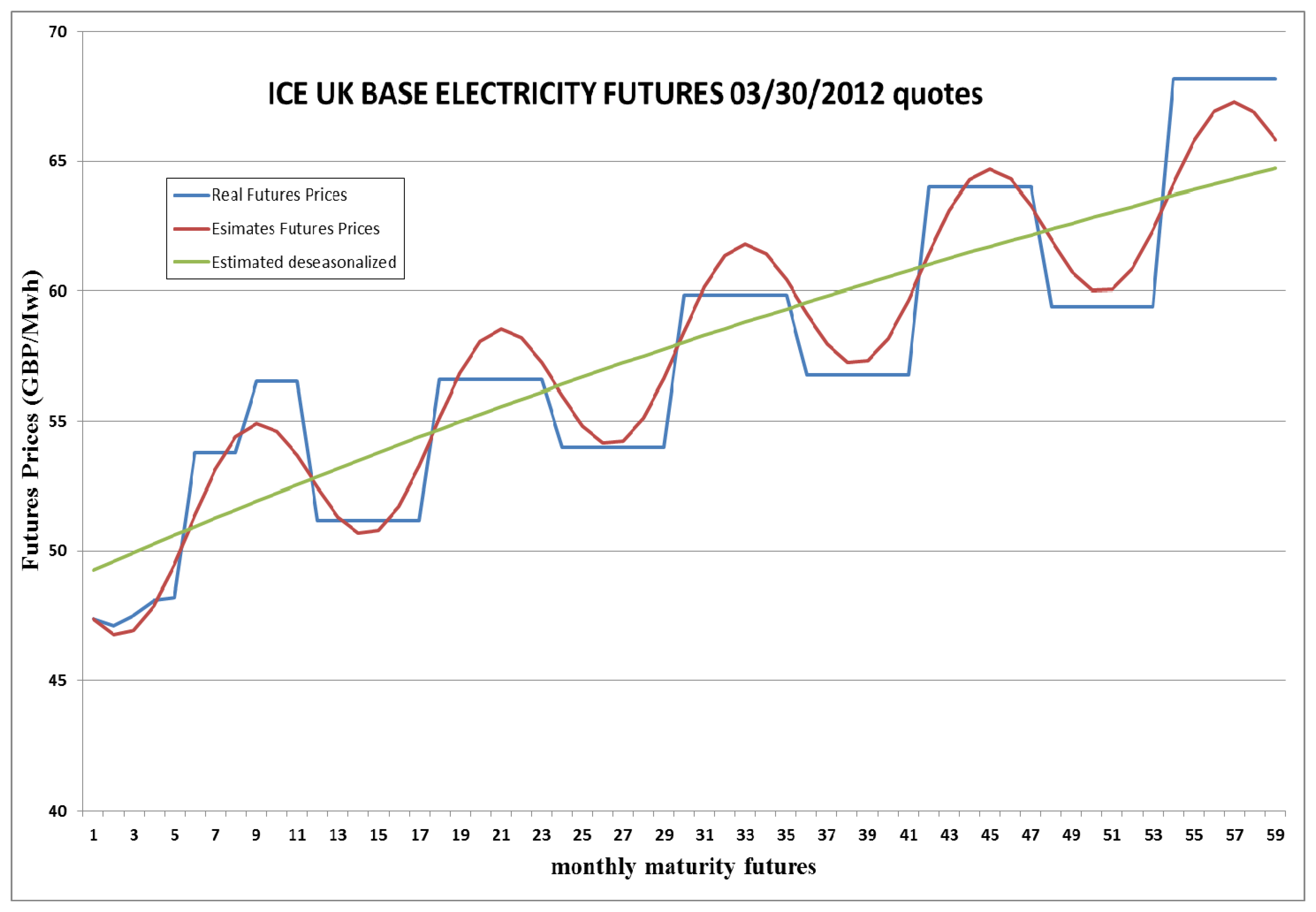
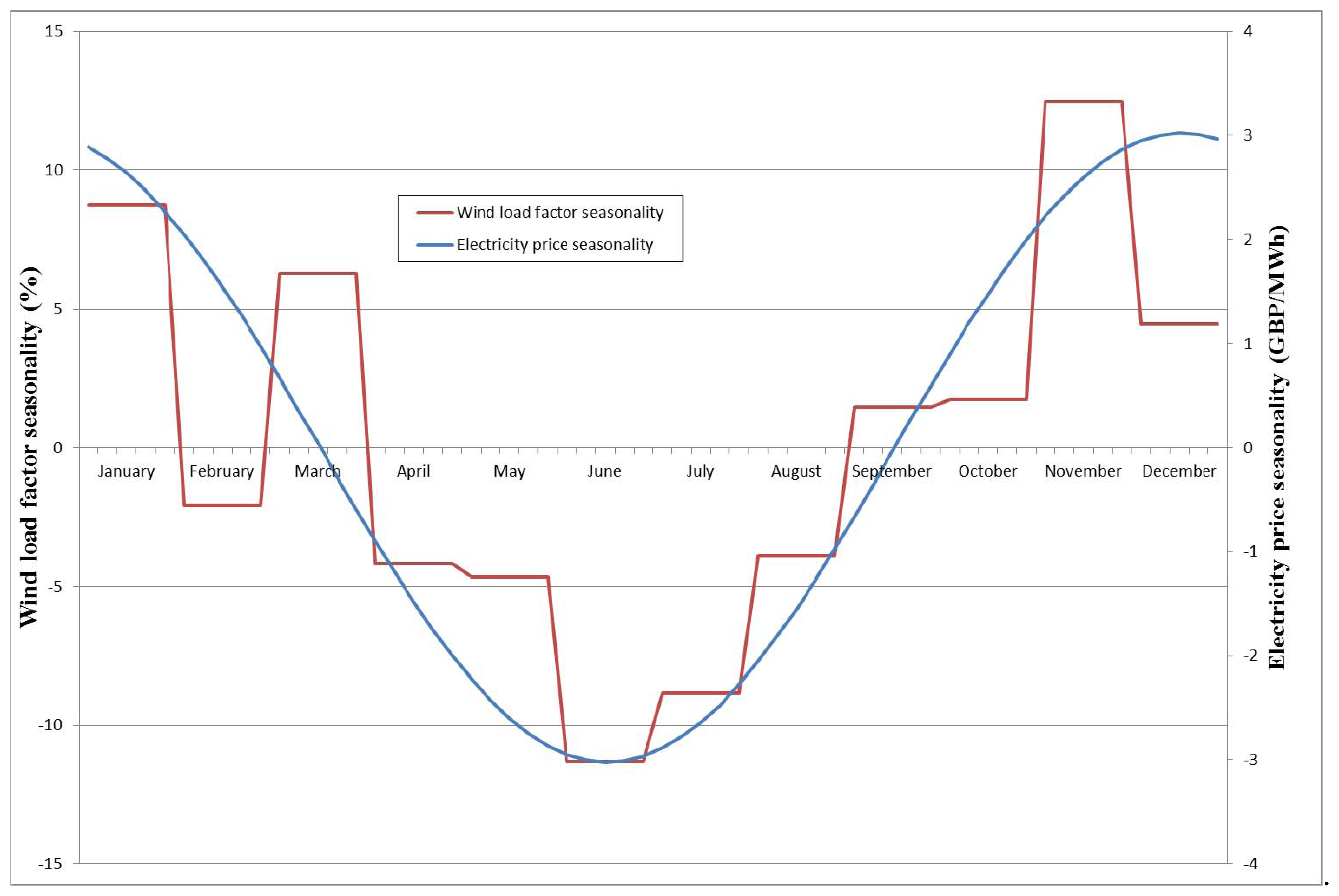
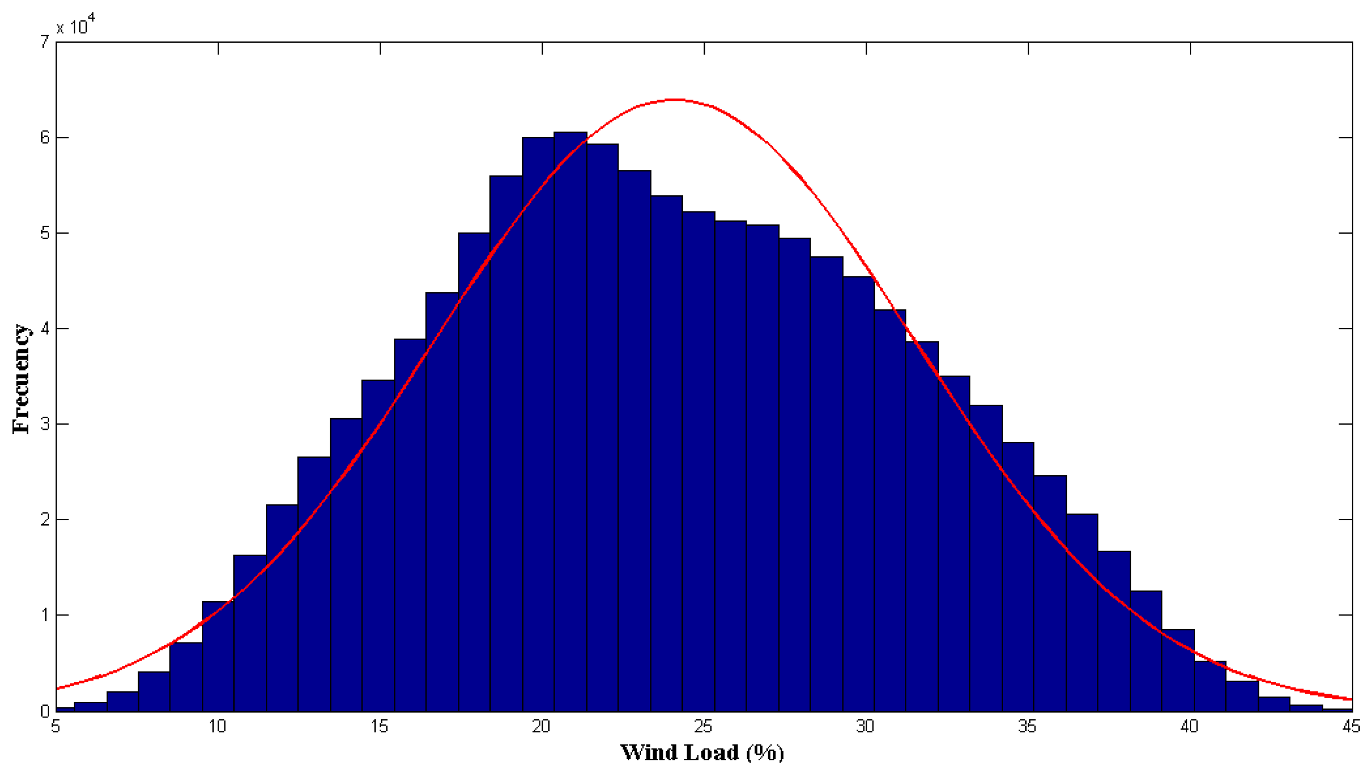


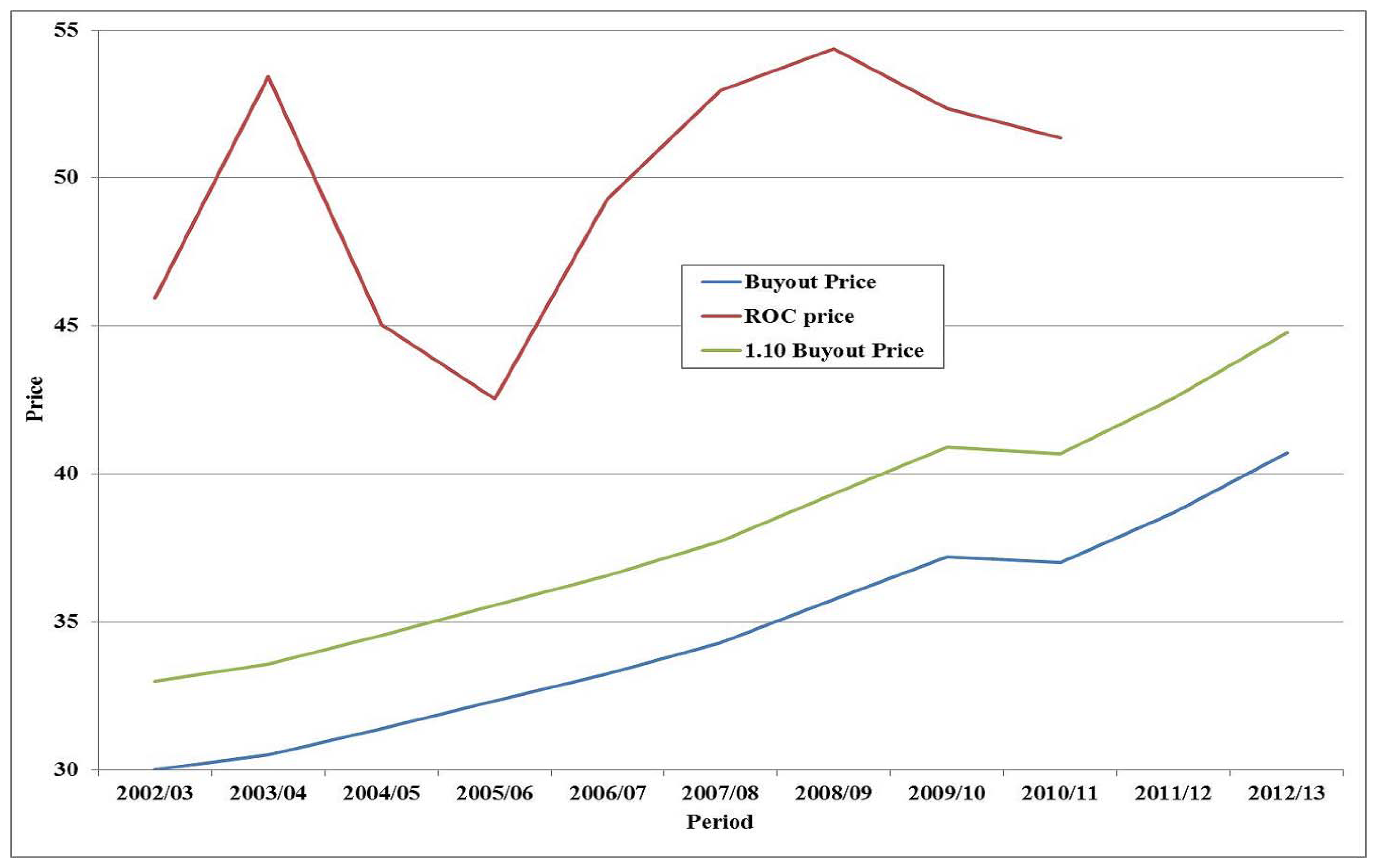
| Summary statistics | |||
|---|---|---|---|
| Set | Observations | Average price (£/MWh) | Standard deviation |
| All contracts | 26,057 | 54.88 | 7.69 |
| 1 Month | 604 | 44.95 | 6.03 |
| 6 Months | 604 | 47.53 | 7.31 |
| 12 Months | 594 | 49.68 | 5.60 |
| 24 Months | 422 | 54.80 | 3.82 |
| 36 Months | 422 | 58.34 | 4.21 |
| 48 Months | 422 | 61.83 | 4.30 |
| 60 Months | 25 | 68.59 | 0.59 |
| Contract specifications | |||
| Delivery period | Contract size (MWh) | ||
| March (1 less hour clock change): | 35 days × 24 h − 1 = 839 MWh | ||
| February (leap year): | 29 days × 24 h = 696 MWh | ||
| January, February, April, May, July, August, November: | 28 days × 24 h = 672 MWh | ||
| June, September, December: | 35 days × 24 h = 840 MWh | ||
| October (1 extra hour clock change): | 28 days × 24 h + 1 = 673 MWh | ||
Source: ICE Futures Europe: “UK Base Electricity Futures”.
| Parameter | Estimate | Standard error | t-ratio | p-value |
|---|---|---|---|---|
| kE + λE | 0.1134 | 0.001939 | 58.47 | 0.000 |
| 85.9128 | 0.542854 | 158.3 | 0.000 | |
| γ | 3.02281 | 0.020658 | 146.3 | 0.000 |
| φ (years) | 0.03139 | 0.0010417 | 30.13 | 0.000 |
| Dummy | Coeff. | t-ratio |
|---|---|---|
| g(1) | 8.7442 | 9.1273 |
| g(2) | −2.0608 | −2.1511 |
| g(3) | 6.2505 | 6.5244 |
| g(4) | −4.1947 | −4.8954 |
| g(5) | −4.6595 | −5.4378 |
| g(6) | −11.3065 | −13.1949 |
| g(7) | −8.8292 | −10.3039 |
| g(8) | −3.8895 | −4.5392 |
| g(9) | 1.4574 | 1.7009 |
| g(10) | 1.7411 | 2.0320 |
| g(11) | 12.4732 | 14.5565 |
| g(12) | 4.4757 | 5.2232 |
| Years | E(Bt) | E(Rt) | E(ROCt) |
|---|---|---|---|
| 0 | 36.99 | 10.65 | 51.34 |
| 5 | 42.19 | 9.43 | 55.84 |
| 10 | 48.12 | 8.35 | 61.28 |
| 15 | 54.88 | 7.39 | 67.76 |
| 20 | 62.59 | 6.55 | 75.40 |
| Variables | Electricity price | Wind load | ROC price |
|---|---|---|---|
| Electricity price | 1.0000 | 0.1038 | 0.2008 |
| Wind load | 0.1038 | 1.0000 | −0.0071 |
| ROC price | 0.2008 | −0.0071 | 1.0000 |
| Location | Online year | Size (MW) | Overnight cost ($/kW) | Variable O&M cost | Fixed O&M cost (2010$/kW) |
|---|---|---|---|---|---|
| Onshore | 2011 | 100 | 2437 | 0 | 28.07 |
| Offshore | 2015 | 400 | 5974 | 0 | 53.33 |
| Currency units | Overnight cost | Fixed annual O&M cost | Total Cost (20 years) |
|---|---|---|---|
| $M | 121.85 | 1.40 | 149.92 |
| £M | 78.567 | 0.905 | 96.667 |
| Tariff p (£/MWh) | Exact V (£) | Monte Carlo V (£) |
|---|---|---|
| 50 | 86,654,277 | 86,638,266 |
| 60 | 103,985,132 | 103,965,920 |
| 70 | 121,315,988 | 121,293,573 |
| 80 | 138,646,843 | 138,621,226 |
| 90 | 155,977,698 | 155,948,880 |
| ρEW | Monte Carlo V (£) | Exact V (£) | Difference |
|---|---|---|---|
| 0 | 122,196,833 | 122,745,535 | −548,702 |
| 0.1038 | 122,262,434 | - | - |
| 0.2 | 122,314,986 | - | - |
| p (£/MWh) | p = 5 | p = 10 | p = 15 | p = 20 | p = 25 | p = 30 | p = 40 | p = 50 |
|---|---|---|---|---|---|---|---|---|
| Present value (£M) | 130.9 | 139.5 | 148.2 | 156.9 | 165.5 | 174.2 | 191.5 | 208.8 |
| i | Term = 10 years | Term = 20 years | ||
|---|---|---|---|---|
| Present value | Subsidy | Present value | Subsidy | |
| 0.0205 | 75.0 | 0.0 | 75.0 | 0.0 |
| 0.01 | 70.9 | 4.0 | 67.7 | 7.2 |
| 0.00 | 67.1 | 7.8 | 60.8 | 14.1 |
| i | Term = 10 years | Term = 20 years | ||
|---|---|---|---|---|
| Present value | Add. cost | Present value | Add. cost | |
| 0.0205 | 75.0 | 0.0 | 75.0 | 0.0 |
| 0.03 | 78.7 | 3.7 | 81.6 | 6.6 |
| 0.04 | 82.6 | 7.6 | 88.6 | 13.6 |
| 0.05 | 86.6 | 11.6 | 95.8 | 20.8 |
| 0.06 | 90.6 | 15.6 | 102.9 | 27.9 |
| Case | pu | pm | pd |
|---|---|---|---|
| Normal | |||
| High X (pu < 0) | |||
| Low X (pd < 0) |
| I | Investment value | Continuation value | Option value |
|---|---|---|---|
| I = £75 M | 47.2 | 59.0 | 59.0 |
| I = £96.667 M | 25.6 | 40.4 | 40.4 |
| I = £100 M | 22.2 | 37.5 | 37.5 |
| I = £125 M | −2.8 | 18.3 | 18.3 |
| I = £150 M | −27.8 | 7.7 | 7.7 |
| Subsidy | S = £5 M | S = £10 M | S = £15 M | S = £20 M |
|---|---|---|---|---|
| I* | £19.3 M | £61.9M | £98.1 M | £122.4 M |
| I | Investment value | Continuation value | Option value | |||
|---|---|---|---|---|---|---|
| p = 20 | p = 10 | p = 20 | p = 10 | p = 20 | p = 10 | |
| I = £75 M | 81.9 | 64.6 | 89.1 | 74.0 | 89.1 | 74.0 |
| I = £96.667 M | 60.2 | 42.9 | 70.1 | 55.2 | 70.1 | 55.2 |
| I = £100 M | 56.9 | 39.6 | 67.2 | 52.4 | 67.2 | 52.4 |
| I = £125 M | 31.9 | 14.6 | 45.6 | 31.1 | 45.6 | 31.1 |
| I = £150 M | 6.9 | −10.4 | 24.6 | 14.0 | 24.6 | 14.0 |
| I | Investment value | Continuation value | Option value |
|---|---|---|---|
| I = £75 M | 153.2 | 163.1 | 163.1 |
| I = £96.667 M | 131.5 | 143.3 | 143.3 |
| I = £100 M | 128.2 | 140.3 | 140.3 |
| I = £125 M | 103.2 | 117.5 | 117.5 |
| I = £150 M | 78.2 | 94.9 | 94.9 |
| I | Investment value | Continuation value | Option value | ||||||
|---|---|---|---|---|---|---|---|---|---|
| T = 5 | T = 2.5 | T = 1 | T = 5 | T = 2.5 | T = 1 | T = 5 | T = 2.5 | T = 1 | |
| I = £75 M | 47.2 | 47.2 | 47.2 | 54.7 | 51.6 | 49.2 | 54.7 | 51.6 | 49.2 |
| I = £96.667 M | 25.6 | 25.6 | 25.6 | 34.9 | 30.9 | 28 | 34.9 | 30.9 | 28 |
| I = £100 M | 22.2 | 22.2 | 22.2 | 31.8 | 27.7 | 24.7 | 31.8 | 27.7 | 24.7 |
| I = £125 M | −2.8 | −2.8 | −2.8 | 11.8 | 7.4 | 3.7 | 11.8 | 7.4 | 3.7 |
| I = £150 M | −27.8 | −27.8 | −27.8 | 3.3 | 1 | 0.1 | 3.3 | 1 | 0.1 |
| S (£M) | S = £1 M | S = £2 M | S = £3 M | S = £4 M | S = £5 M | S = £10 M | S = £15 M | S = £20 M |
|---|---|---|---|---|---|---|---|---|
| I* (£M) | £26.0 M | £77.7 M | £115.0 M | £119.1 M | £122.6 M | £130.7 M | £136.4 M | £142.0 M |
| I | Investment value | Continuation value | Option value | |||
|---|---|---|---|---|---|---|
| σE = 0.20 | σE = 0.10 | σE = 0.20 | σE = 0.10 | σE = 0.20 | p = 10 | |
| I = £75 M | £47.2 M | £47.2 M | £57.7 M | £55.5 M | £57.7 M | £55.5 M |
| I = £96.667 M | £25.6 M | £25.6 M | £39.1 M | £37.0 M | £39.1 M | £37.0 M |
| I = £100 M | £22.3 M | £22.3 M | £36.3 M | £34.2 M | £36.3 M | £34.2 M |
| I = £125 M | −£2.8 M | −£2.8 M | £16.2 M | £13.4 M | £16.2 M | £13.4 M |
| I = £150 M | −£27.8 M | −£27.8 M | £5.1 M | £1.2 M | £5.1 M | £1.2 M |
| I0 | £75 M | £96.667 M | £100 M | £125 M | £150 M |
|---|---|---|---|---|---|
| Continuation value | 63.9 | 47.2 | 44.6 | 25.8 | 12.0 |
| Option value | 63.9 | 47.2 | 44.6 | 25.8 | 12.0 |
| Values | αI = 0 | αI = −0.0108 | |||
|---|---|---|---|---|---|
| αV = 0 | αV = −0.02 | αV = 0 | αV = −0.02 | ||
| premium = 20 | Investment value | 60.2 | 60.2 | 60.2 | 60.2 |
| Continuation value | 70.1 | 66.6 | 76.5 | 72.4 | |
| Option value | 70.1 | 66.6 | 76.5 | 72.4 | |
| premium = 10 | Investment value | 42.9 | 42.9 | 42.9 | 42.9 |
| Continuation value | 55.2 | 53.3 | 61.8 | 59.6 | |
| Option value | 55.2 | 53.3 | 61.8 | 59.6 | |
© 2014 by the authors; licensee MDPI, Basel, Switzerland. This article is an open access article distributed under the terms and conditions of the Creative Commons Attribution license (http://creativecommons.org/licenses/by/3.0/).
Share and Cite
Abadie, L.M.; Chamorro, J.M. Valuation of Wind Energy Projects: A Real Options Approach. Energies 2014, 7, 3218-3255. https://doi.org/10.3390/en7053218
Abadie LM, Chamorro JM. Valuation of Wind Energy Projects: A Real Options Approach. Energies. 2014; 7(5):3218-3255. https://doi.org/10.3390/en7053218
Chicago/Turabian StyleAbadie, Luis M., and José M. Chamorro. 2014. "Valuation of Wind Energy Projects: A Real Options Approach" Energies 7, no. 5: 3218-3255. https://doi.org/10.3390/en7053218
APA StyleAbadie, L. M., & Chamorro, J. M. (2014). Valuation of Wind Energy Projects: A Real Options Approach. Energies, 7(5), 3218-3255. https://doi.org/10.3390/en7053218