1. Introduction
The building sector represents 40% of the European Union’s total energy consumption. Therefore reducing energy consumption is a priority of the climate and energy package called “20-20-20”. The European Directive 31/2010 [
1] upholds the concept of zero or nearly zero-energy constructions (ZEBs or n-ZEBs) which are increasingly becoming more common throughout Europe. By 31 December 2020, all new buildings must be n-ZEBs, and in particular those occupied and owned by public authorities must comply with the same criteria by 31 December 2018. New buildings must fulfill these requirements before construction starts, looking at high efficiency envelopes, the installation of renewable energy systems, heat pumps and cogeneration systems.
Many studies have analyzed several types of high energetic efficiency external walls for ZEBs; in particular in the Mediterranean climate, Baglivo
et al. [
2,
3] carried out an analysis through the combination of various materials, in terms of steady thermal transmittance, periodic thermal transmittance, decrement factor, time shift, areal heat capacity, thermal admittance, surface mass, thickness.
In the literature it was already demonstrated that the substitution of traditional air heat pumps coupled with Ground Source Heat Pump (GSHPs) results in a good reduction of CO
2 emissions [
4] and a good return of the investment in the case of large size applications such as commercial buildings [
5]. The reduction of consumption and emissions with respect to traditional heat pump is due to the increase of the Coefficients of Performance (COP) in GSHP system, both in summer and in winter [
6]. Energy studies on these features [
7], together with their flexible application, noise reduction and space preservation were the engine of their success and diffusion [
8,
9].
Desideri
et al. [
10] showed that the operating costs necessary to heat the building with the GSHP, are lower than the ones for heating the building with a natural gas boiler. Previous studies are mainly focused on the use of horizontal water ground heat exchangers [
11,
12,
13]. Demir
et al. [
11] carried out an experimental study to test the validity of the model; experimental and numerical simulation results, calculated using experimental water inlet temperatures, were compared. Congedo
et al. [
12] compared different configurations of horizontal water ground heat exchangers in order to define the system performance. Wu
et al. [
13] investigated both experimentally and numerically the thermal performance of slinky heat exchangers of horizontal-coupled slinky GSHP in a UK climate. Few studies concern the analysis of horizontal air ground heat exchangers. In [
14] the experimental measurements and numerical simulation of an air ground source heat exchanger operating at a cold climate for a passive house ventilation system were reported.
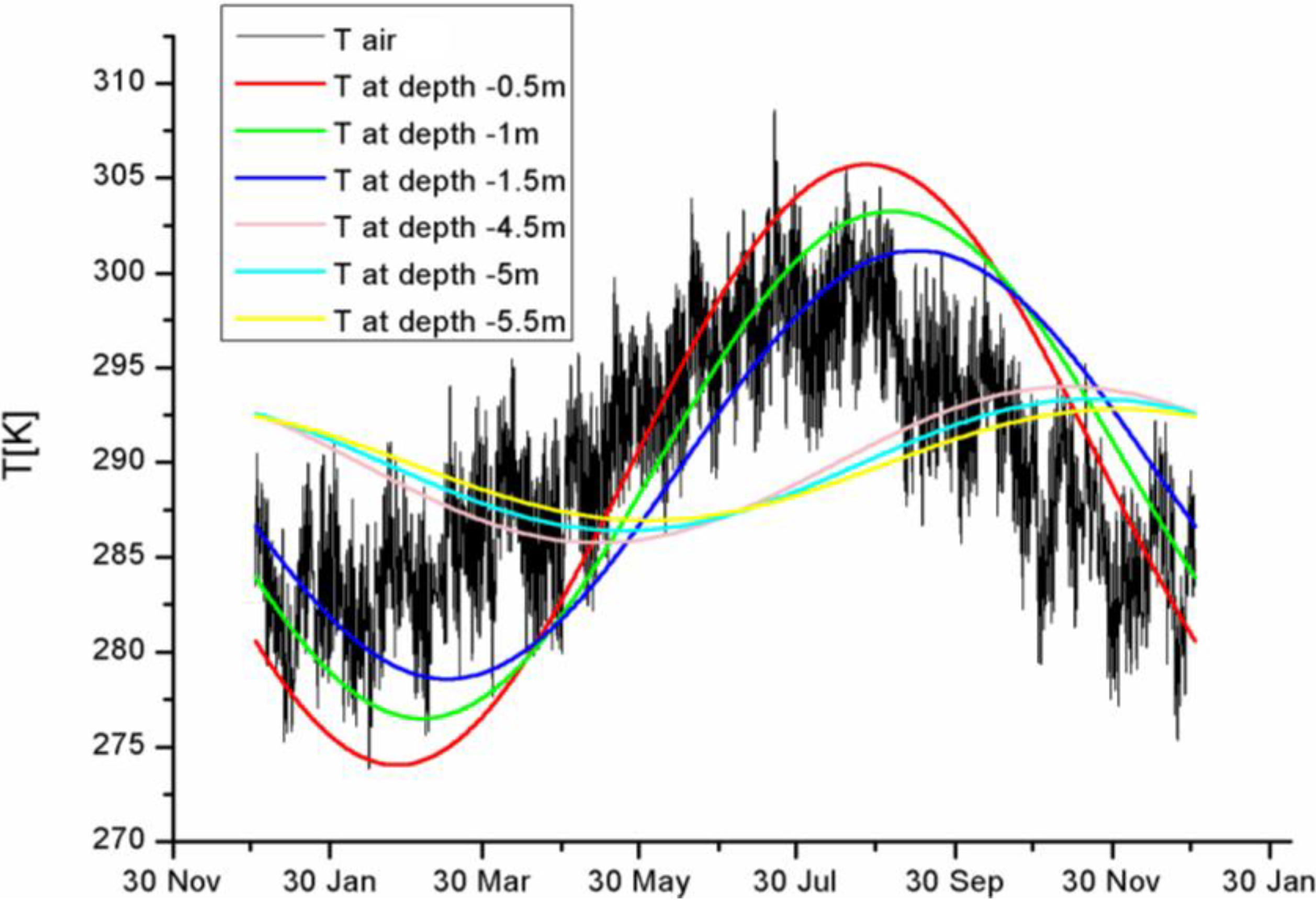
Figure 1 shows the behavior of the outside air temperature and the ground temperature varying the depth along year 2002 by a climatic station located in the city of Lecce (Italy). Ground temperature variations are damped and phase delayed, compared to the outside air temperature ones, because of the ground thermal inertia and heat capacity (higher than air). Consequently, the ground temperature, below a certain depth, remains relatively constant throughout the year. The seasonal delay that depends on the depth and the ground composition can be as long as some weeks. Therefore, at a sufficient depth, the ground temperature is higher than that of the outside air in winter and is lower in summer. The difference in temperature between the outside air and the ground can be used as a preheating means in winter and pre-cooling in summer by a HAGHE. The idea of preheating or cooling the air by the ground is already treated by Wrobel
et al. [
15,
16].
Figure 1.
Ground temperature distribution for λ = 2 W/(m K), measured by a climatic station located in the city of Lecce (Italy).
Figure 1.
Ground temperature distribution for λ = 2 W/(m K), measured by a climatic station located in the city of Lecce (Italy).
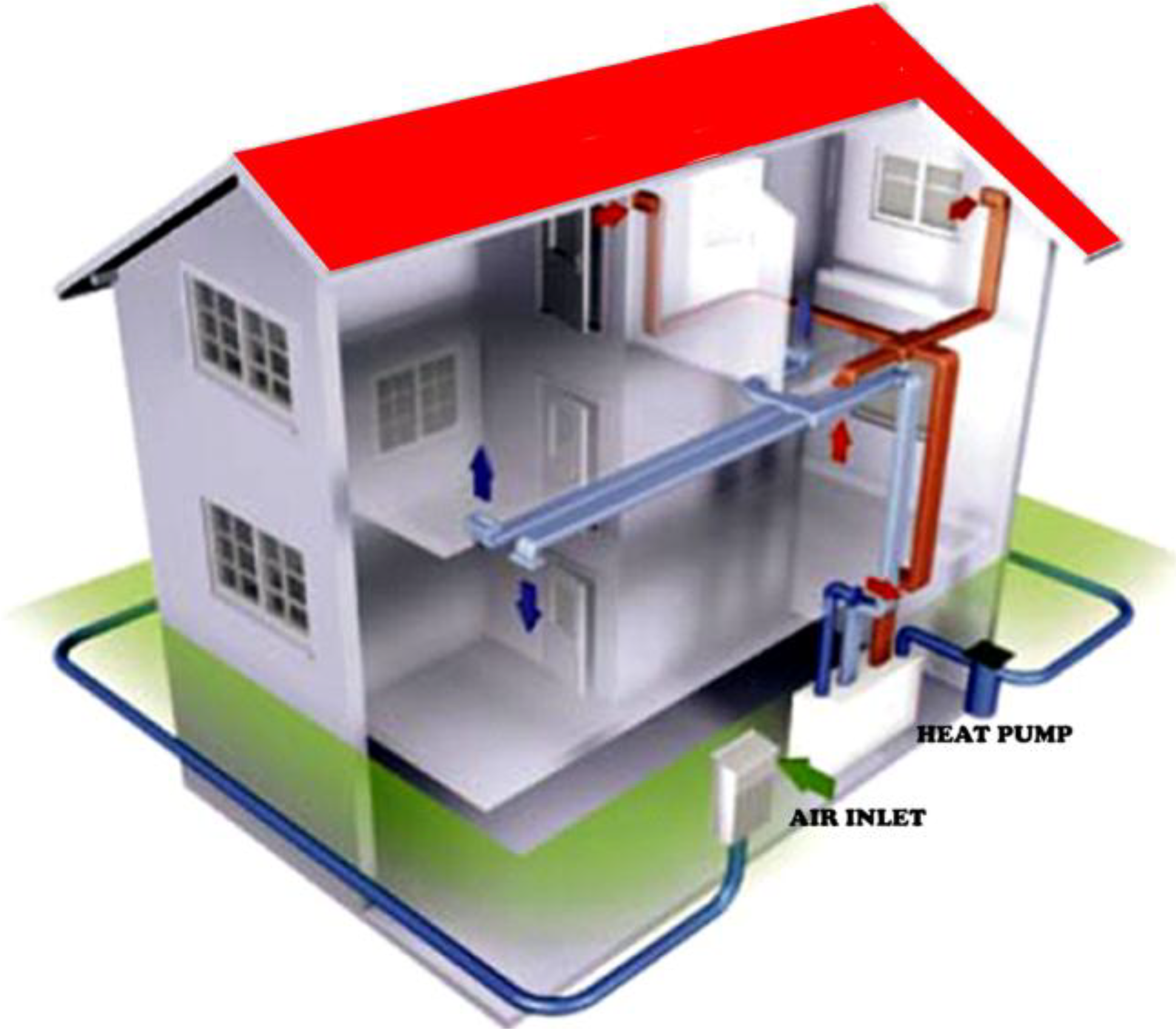
HAGHE’s basically consist of pipes which are buried in the ground at the depth of about 2 m, coupled with an air system which forces the outside air through the pipes and eventually mixes it with the indoor air of the building (see
Figure 2). For a large number of applications it is necessary to know the influence of each parameter on the thermal performance of HAGHE as well as the pipes layout and the ground properties.
Figure 2.
HAGHE integrated with mechanical ventilation or heat pump.
Figure 2.
HAGHE integrated with mechanical ventilation or heat pump.
The present work aims to demonstrate that the geothermal heat exchanger horizontal air-to-ground (HAGHEs) can also show good performance in terms of high efficiency of the total system with a low environmental impact, operating on the ventilation air, in particular for ZEB buildings. The main cost for the installation of HAGHEs is comparable to GSHPs cost, due to drilling cost [
17,
18]. This study shows the thermal behavior of HAGHEs placed in south of Italy, in particular, in the city of Lecce. Some topics are discussed about the heat fluxes transferred to and from the soil and the temperature modifications of the soil around the heat exchanger, both in summer and winter.
2. CFD Numerical Analysis
All the simulations were performed with the CFD ANSYS FLUENT Release 14.0, which uses the control volume method [
19]. Unsteady Reynolds-Averaged Navier-Stokes equations were solved with a second order implicit transient scheme in combination with the realizable k-ε model [
20] with enhanced wall treatment with thermal effect option. The k-ε model is appropriate for wall-bounded and internal flows with small mean pressure gradients [
21]. As a solution method pressure—velocity coupling was chosen with a Semi-Implicit Method for Pressure-Linked Equations (SIMPLE) algorithm. The CFD code main setup parameters are reported in
Table 1. The numerical study was carried out in unsteady conditions with a 3D structured mesh by previous analysis [
22,
23]. All the geometry independent parameters were the same for all the layouts considered. The heat exchangers were simulated under different operating conditions.
Table 1.
Details of CFD setting.
Table 1.
Details of CFD setting.
| Element | Description |
|---|
| Mesh Elements | 3D Structured mesh, hexahedral elements |
| Numbers of cells/faces/nodes | 171.820/530.731/186.934 |
| Solver | 3D unsteady, pressure based |
| Numerical Scheme | Segregated |
| Linearization | Implicit |
| Discretization Scheme | |
| Pressure | PRESTO! |
| Pressure velocity coupling | SIMPLE |
| Momentum, turbulence kinetic energy, turbulence dissipation rate | 2nd order upwind |
| Fluid | Ideal gas |
| Turbulence model | Realizable k-ε |
| Time step | 1 s |
2.1. Geometrical Model
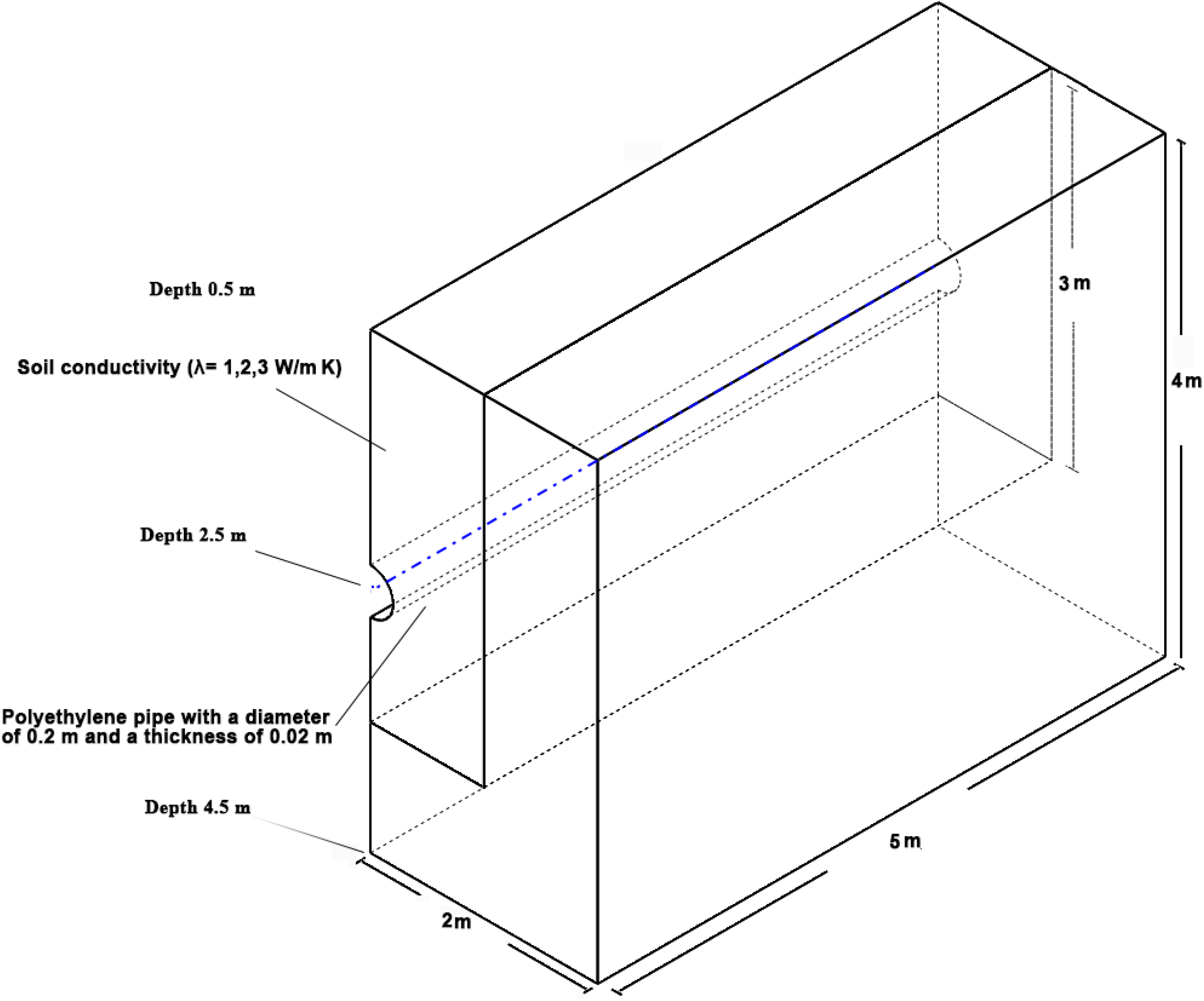
A 3D structured grid was generated by means of the grid generator GAMBIT. The 3D analysis used a parallelepiped domain of 5.0 m × 2.0 m × 4.0 m (length × width × depth) with 200 mm diameter polyethylene (PE) semi-cylinder pipe, thickness 20 mm, at a depth of 2.5 m. Due to the symmetry of the investigated configuration an half of the ground-pipe heat exchanger was discretized and simulated (see
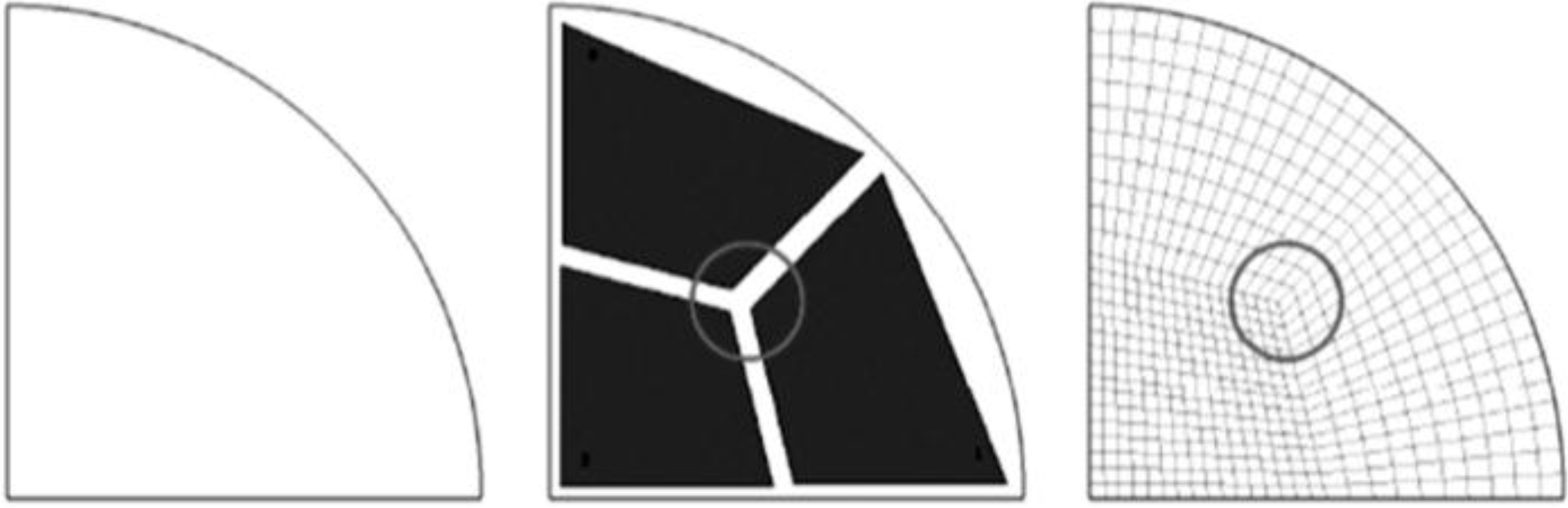
Figure 3). The structured grid is composed of hexahedral cells, stretched towards the curved lateral surface of the semi-cylinder into the ground parallelepiped. The structured hexahedral mesh is typically obtained from a coarse structure (super-blocks) that divides the 2D/3D domain in parallelograms/parallelepipeds. How these super-blocks are related with each other is called topology. Depending on how the different blocks are joined with each other to cover the whole domain, are defined different topologies.
Figure 4 shows the mesh of a quarter of cross section of the pipe, from the three parallelogram-shaped super-blocks, we obtain the topology “O-grid”.
Figure 3.
Simulated geometry of HAGHE due to symmetry of numerical model.
Figure 3.
Simulated geometry of HAGHE due to symmetry of numerical model.
Figure 4.
Mesh of a quarter of cross section of the pipe.
Figure 4.
Mesh of a quarter of cross section of the pipe.
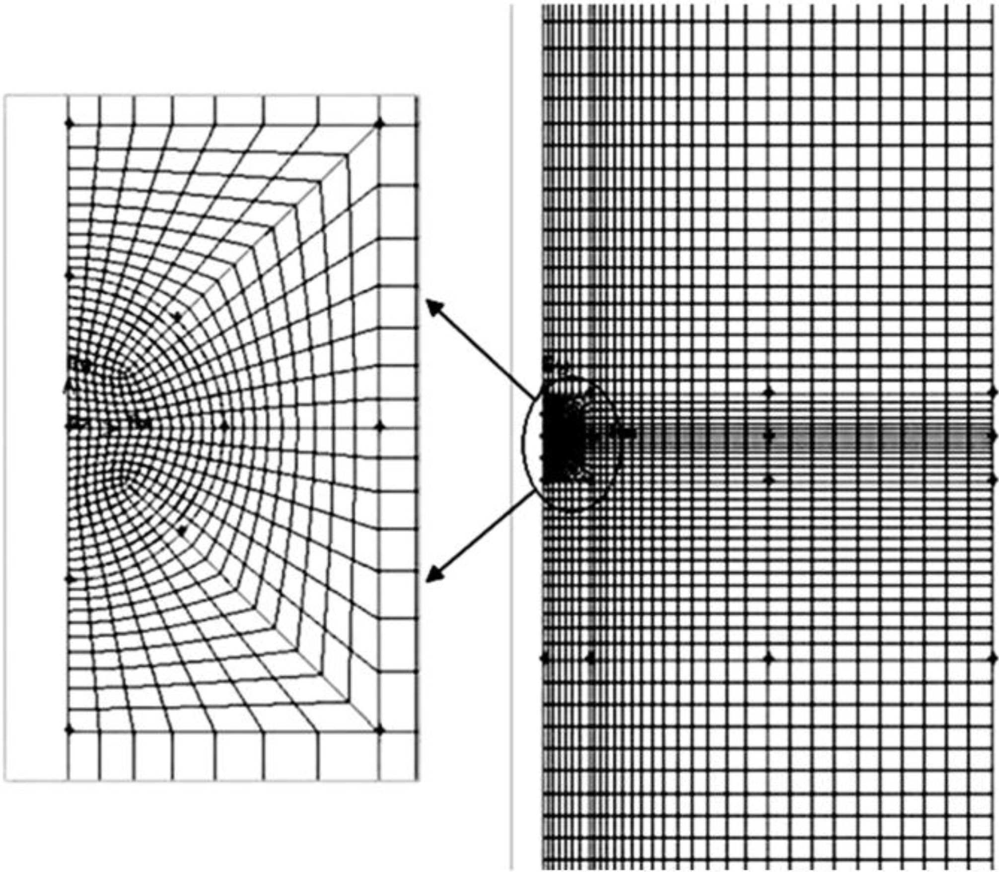
It was considered to discretize the area more accurate from the point of view of fluid dynamics, around the pipe, where the highest gradients are expected, using a structured mesh with hexahedral elements, towards the curved side surface of the semi-pipe. This leads to significant advantages of the numerical solution, which present a higher accuracy, and a numbering more effective. Then, a finer mesh is used (to check the accuracy of the solution) near the ground-pipe interface, which slopes down to a coarser mesh in the area far from the semi-cylinder, as shown in
Figure 5. As can be clearly observed, to obtain a mesh of good quality, was strictly observed the principle of gradual change in the size of the cells; it was, in fact, imposed a “growth rate” quite low to the cells adjacent to one another, by ensuring that each cell had never more than triple in size of the previous cell.
Figure 5.
Details of the mesh, on left around the pipe, on right of cross section of the simulated domain.
Figure 5.
Details of the mesh, on left around the pipe, on right of cross section of the simulated domain.
2.2. Boundary Conditions
To model the temperature profile into the ground in function of the depth (
z) and time (
t), the function in Equation (1) was used [
24,
25], because of the interactions of the soil with sun radiation, wind and air temperature during all the year. The values of main properties of the materials used in the simulations and of the constants used in Equation (1) are reported in
Table 2 and
Table 3, respectively.
Table 2.
Main properties of the materials used in the simulations.
Table 2.
Main properties of the materials used in the simulations.
| Variable | Pipe (PE) | Ground | Air |
|---|
| ρ (kg/m3) | 946 | 2723.23 | Ideal gas |
| λ (W/(m·K)) | 0.35 | 1; 2; 3 | 0.0242 |
| cp (J/(kg·K)) | 1920 | 837.338 | 1006.43 |
| µ(kg/s) | | | 1.7894 × 10⁻⁵ |
The values of the temperatures in the ground at different depths are reported in
Figure 1 and were used, to set the boundary conditions in the ground, far from the heat exchanger and thus in undisturbed conditions, for the simulations of the operation of the ground heat exchangers, in particular at depths of 0.5 and 4.5 m. The representation by a simple harmonic of the annual cycle of the monthly mean temperature of the soil is sufficiently precise, as demonstrated by previous in-depth analysis [
26,
27].
In Equation (1)
TM is the mean temperature in the year of the climatic zone;
a is the half difference between the maximum and minimum temperatures on soil surface in the year;
τ is the considered period;
tM is the time when the maximum temperature on the ground surface occurs;
DT is the thermal diffusivity of the considered soil. The main assumptions for this equation is that all the physical properties referred to the soil are constant in space and time and thus a homogeneous soil is considered at all depth. This is a not-too-far-from-reality hypothesis because of the depth (maximum 3 m) and the climate zone (south of Italy is temperate climate zone) considered.
where:
Table 3.
Values of the constant used in Equation (1).
Table 3.
Values of the constant used in Equation (1).
| Constant | Value |
|---|
| TM | 16.73°C |
| a | 18.74°C |
| Depth | 2.5 m |
| τ | 365 (1 year) |
| tM | 45 day |
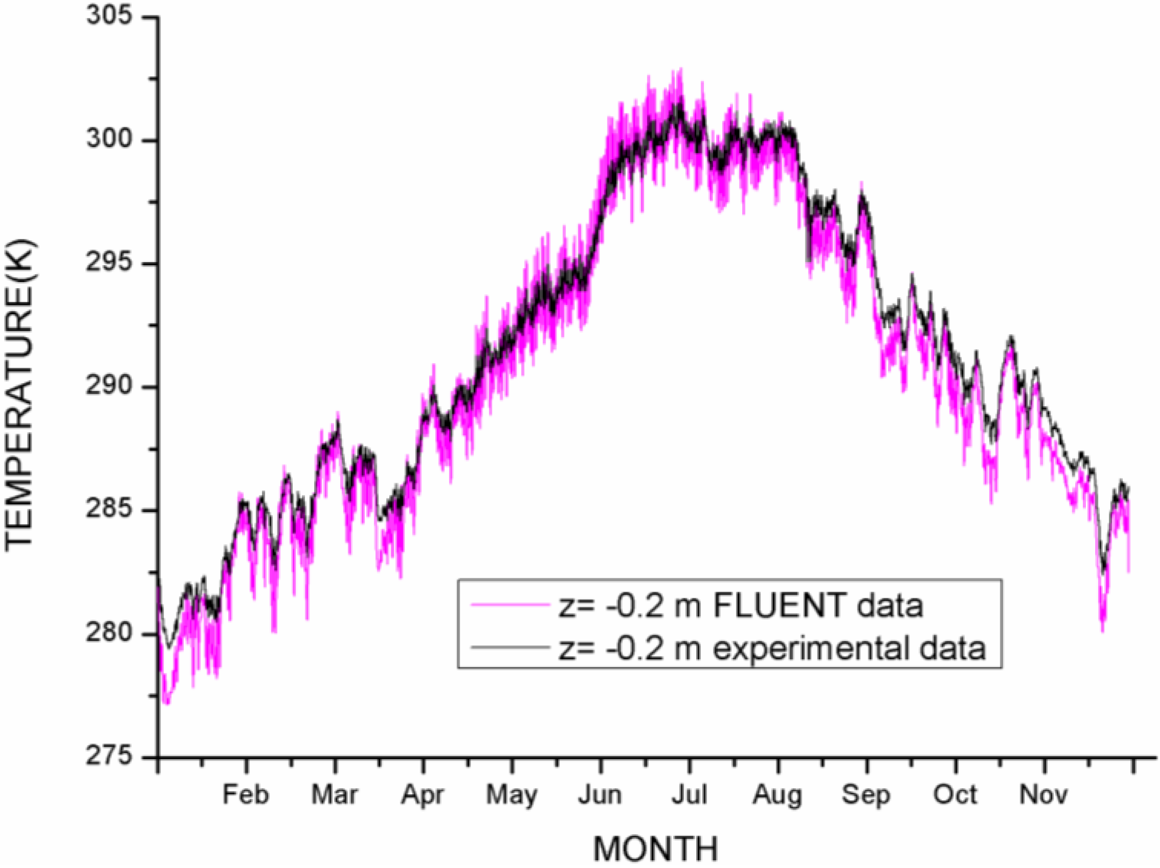
The climatic data used in order to validate the simulation were those recorded in the year 2002 by a climatic station located in the city of Lecce (Italy) at the coordinates: Latitude 40°26'16" North and Longitude 18°14'42" East. The available experimental data were air temperature and underground temperature at two depths (0.1 and 0.2 m) with a time step of an hour, the same data used in a previous work [
5], where a comparison between experimental temperatures recorded in one year at two different depths in the ground with the calculated data by the CFD code was made.
Figure 6 shows the hourly average temperatures at a depth of 0.2 m experimentally measured (black line) and the ones (grey line) calculated by the numerical simulation. The comparison between the two lines confirmed a good choice of the boundary condition for the numerical simulations.
Figure 6.
Comparison between the experimental data and the results from the CFD simulations [
5].
Figure 6.
Comparison between the experimental data and the results from the CFD simulations [
5].
Looking at
Figure 3, the boundary conditions have the following setup. The upper and lower horizontal surfaces have “wall” temperatures imposed by a transient table: the soil temperatures have been imposed at depths 0.5 m and 4.5 m, respectively, varying during the year. The vertical surface close to the semi-pipe is “symmetry” and the other vertical surfaces are “adiabatic walls”.
The performance of the heat exchangers were numerically investigated during the entire year, simulating the heat flux passing through a portion of soil and transmitted to the air in the polyethylene pipe. In
Table 1, the main parameters of the ground properties are shown, supposed homogeneous at all depths. The investigation concerned 3 different soil types: low conductivity soil (λ = 1 W/m·K); medium conductivity soil (λ = 2 W/m·K); high conductivity soil (λ = 3 W/m·K). Weather data relating to a climatic station, located in Lecce, were generated using Meteonorm Version 5 [
28].
Air flow rate was set at four different levels to investigate heat exchanger performance in different operating conditions, in particular the values were 150, 250, 350, 450 m3/h respectively. The inlet air temperature was assumed equal to the external temperature varying hour by hour. The activation period of the heating and cooling system was, in winter, from 15 November to 31 March and each day from 8.00 am to 7.00 pm (typical for offices, factories, etc.), in summer, from 1 June to 31 August and each day from 8.00 am to 7.00 pm.
It is to be emphasized, that the physical problem admits, during the shutdown of the plant, when the input air flow is close to zero, the possibility of “reflux” from the air. The flow of air may, occasionally, go in the opposite direction to that of normal operation. It was, therefore, necessary to set, in the boundary condition, the back flow total temperature; it corresponds to the development of time-dependent temperature of the soil, to the level of burial of the pipe. In this way, the numerical code is able to well manage the back flow, providing the correct values during the period of shutdown of the plant.
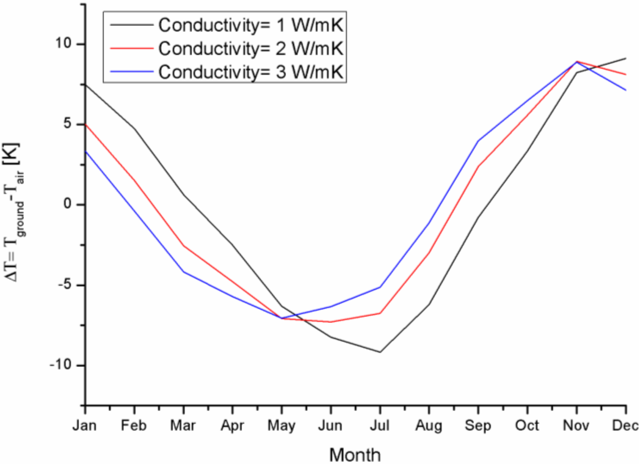
In this work the performance of pre-heating or pre-refreshing the ventilation air using HAGHE is mainly dependent on the difference between the outdoor air temperature and the soil temperature. In South-East Italy, this difference in summer is larger than that in winter, which is the main reason why HAGHE is more effective in summer than in winter.
The analysis shows that, in warm climates, using the HAGHE has its advantages for few hours daily in winter, when the difference between the outdoor air temperature and the soil temperature is small, while it shows significant benefits in the summer for cooling of the ventilation air up to several temperature degrees, when the difference between the ground temperature and the outdoor air temperature is high (see
Figure 7).
2.3. Sensitivity Analysis of Grid Spacing
In order to estimate the error due to spatial discretization a sensitivity analysis of the grid spacing was performed. Congedo
et al. [
29] show the application of the Grid Convergence Index (GCI) in industrial applications. The GCI gives a measure of the percentage the computed value is away from the value of the asymptotic numerical value. For the present work, three different grid refinement levels have been considered. Considering three grid levels, the values for the GCI indexes can be evaluated as follows:
Fs is a factor of safety and for the comparison of three grids is equal to 1.25; with:
where
p is the order of convergence,
h is the grid spacing (minimum value of distance between nodes of grid);
f is the value of the significant parameter chosen for the comparison (the air outlet temperature has been chosen).
Figure 7.
Difference between the ground temperature and the outdoor air temperature.
Figure 7.
Difference between the ground temperature and the outdoor air temperature.
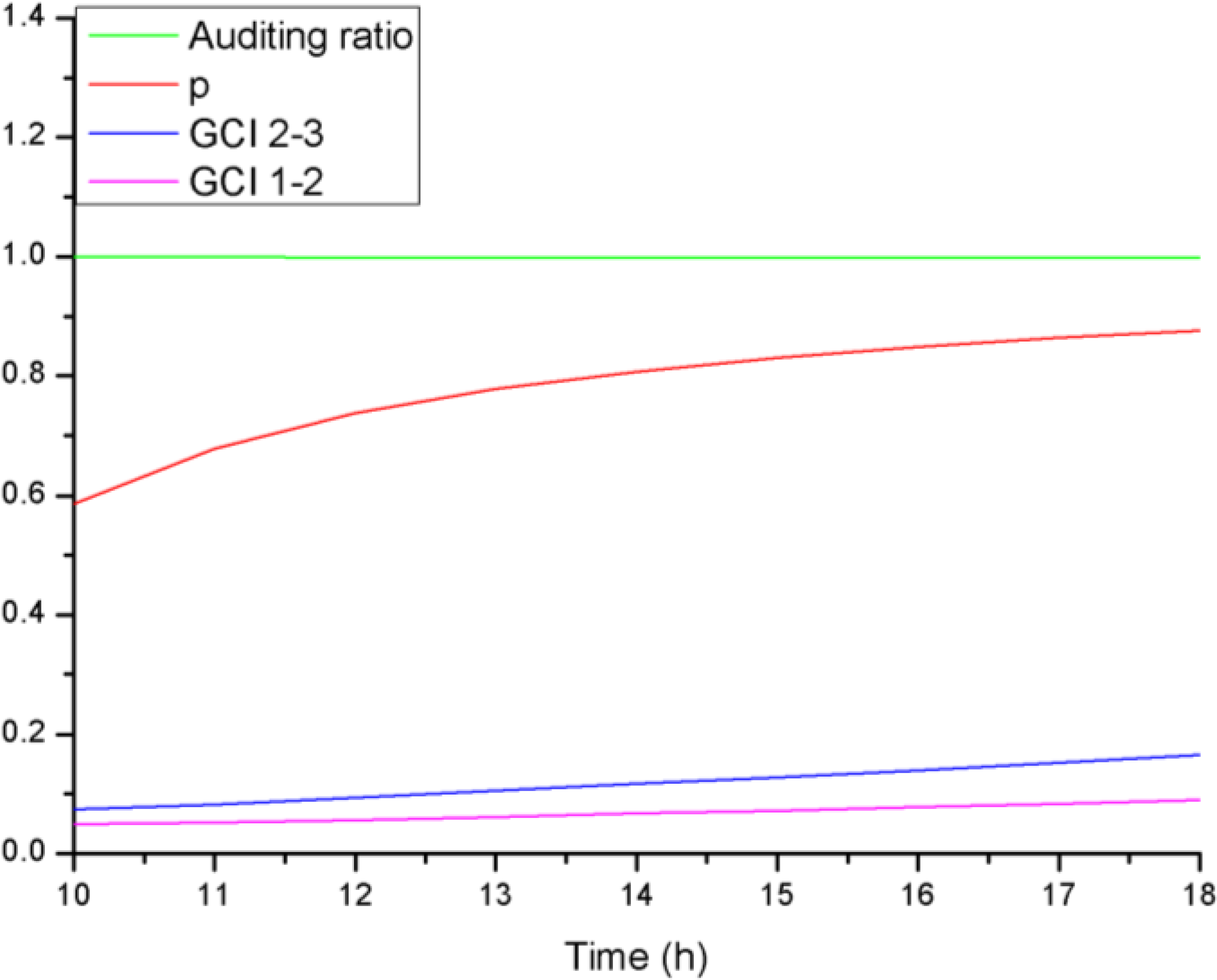
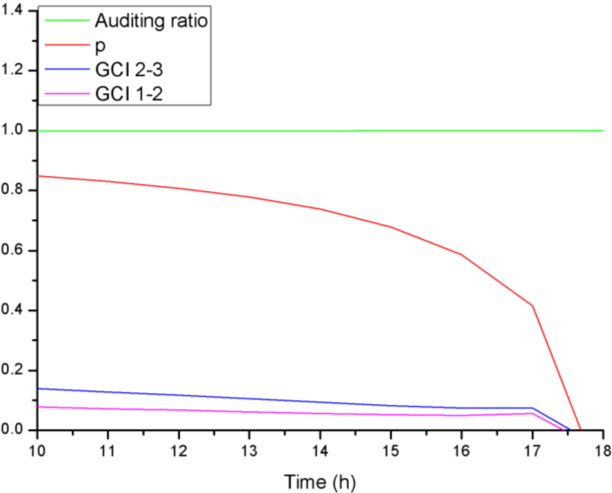
It is important that the solution of the considered grid level is in the asymptotic range; it happens if the following auditing ratio is equal to 1. It means that increasing the number of cells does not change the value of the solution f:
Using the finest grid, the evaluated value of the solution is:
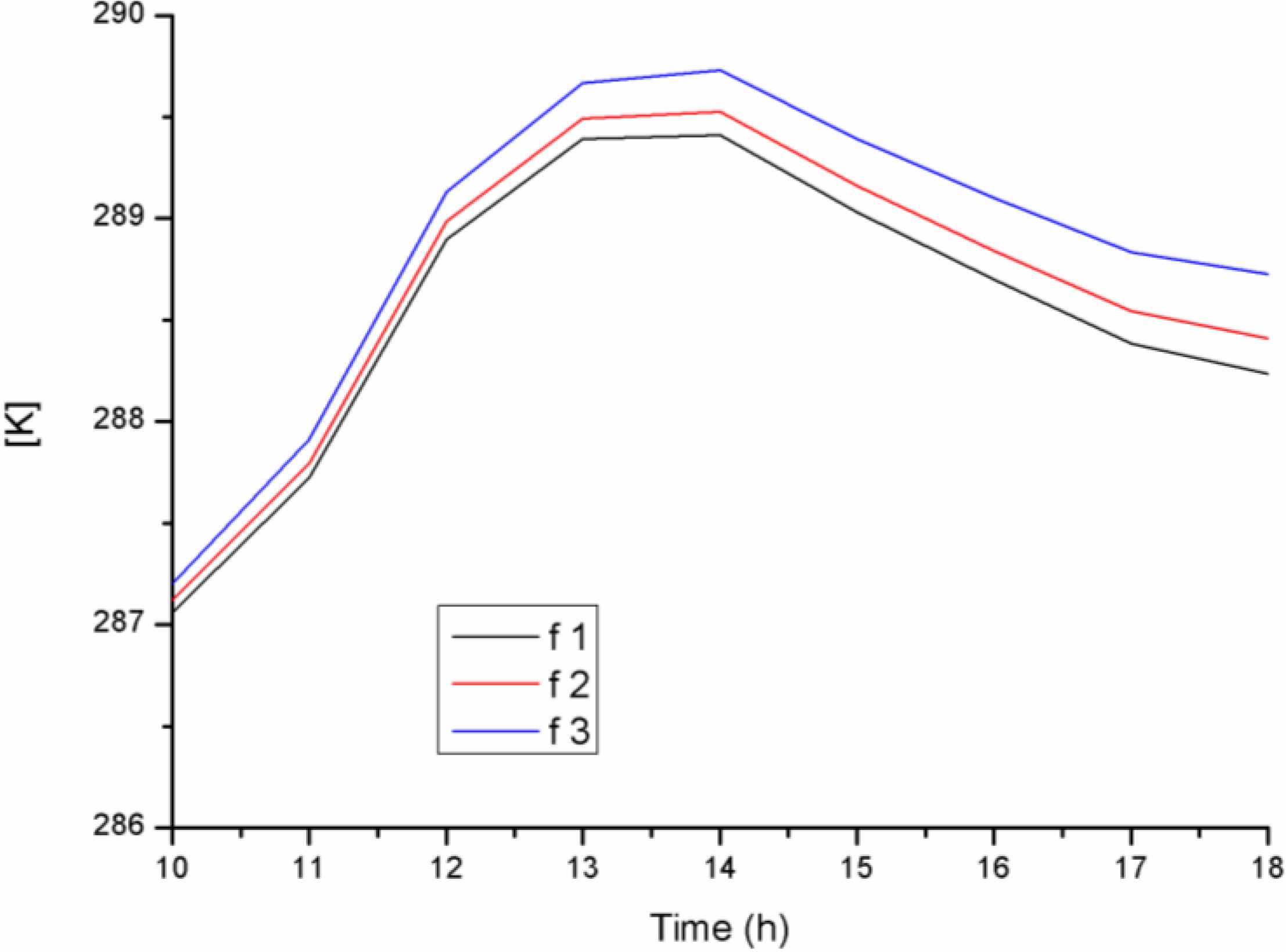
For the present work, the air outlet temperature has been chosen as the comparison parameter. In
Figure 8 such a temperature is plotted as function of time for different grid spaces (
h1= 1.65 mm;
h2 = 3.30 mm;
h3 = 6.60 mm). In detail,
f1 curve represents the temperature calculated with the finest grid,
f2 curve with the medium grid, and
f3 with coarsest one. The curves show a little divergence with increasing time. In
Figure 9 the grid convergence indexes, the order of convergence and the auditing ratio are reported. It is important to verify that the auditing ratio is really close to 1.
Figure 8.
Air outlet temperature is plotted as function of time for different grid spaces.
Figure 8.
Air outlet temperature is plotted as function of time for different grid spaces.
Figure 9.
Grid convergence indexes, auditing ratio and order of convergence vs. time (grid spacing analysis).
Figure 9.
Grid convergence indexes, auditing ratio and order of convergence vs. time (grid spacing analysis).
2.4. Sensitivity Analysis of Time Step
An analogous approach has been taken for the sensitivity analysis of the time step. Looking at
Figure 10 and
Figure 11, again the air outlet temperature has been chosen as the comparison parameter. In detail,
f1 curve represents the temperature calculated with the smallest time step (1 s),
f2 curve with the medium time step (2 s) and
f3 with the greatest time step (4 s). Such curves are overlap completely and the auditing ratio trend in
Figure 11 confirms that the solution is in asymptotic range.
Figure 10.
Air outlet temperature is plotted as function of time for different time steps.
Figure 10.
Air outlet temperature is plotted as function of time for different time steps.
Figure 11.
Grid convergence indexes, auditing ratio and order of convergence vs. time (time step analysis).
Figure 11.
Grid convergence indexes, auditing ratio and order of convergence vs. time (time step analysis).
3. Results
The CFD simulations showed the HAGHE’s behavior (with a length of the pipe, as said, of 5 m) in different operating conditions. As regards the analysis relating to the data of Lecce, the results are represented into four figures: the first three
Figure 12,
Figure 13 and
Figure 14 show the performances of the air-ground heat exchanger in terms of ground and inlet-outlet air temperatures and air-ground thermal power, by varying air flow rate (150 to 450 m
3/h), keeping constant the value of soil conductivity and assuming the temperature of the ground,
Tground, with the plant shut down.
Figure 15 shows, instead, the HAGHE performance by varying the soil conductivity (1, 2, 3 W/m K), keeping constant air flow rate at 350 m
3/h.
Figure 12.
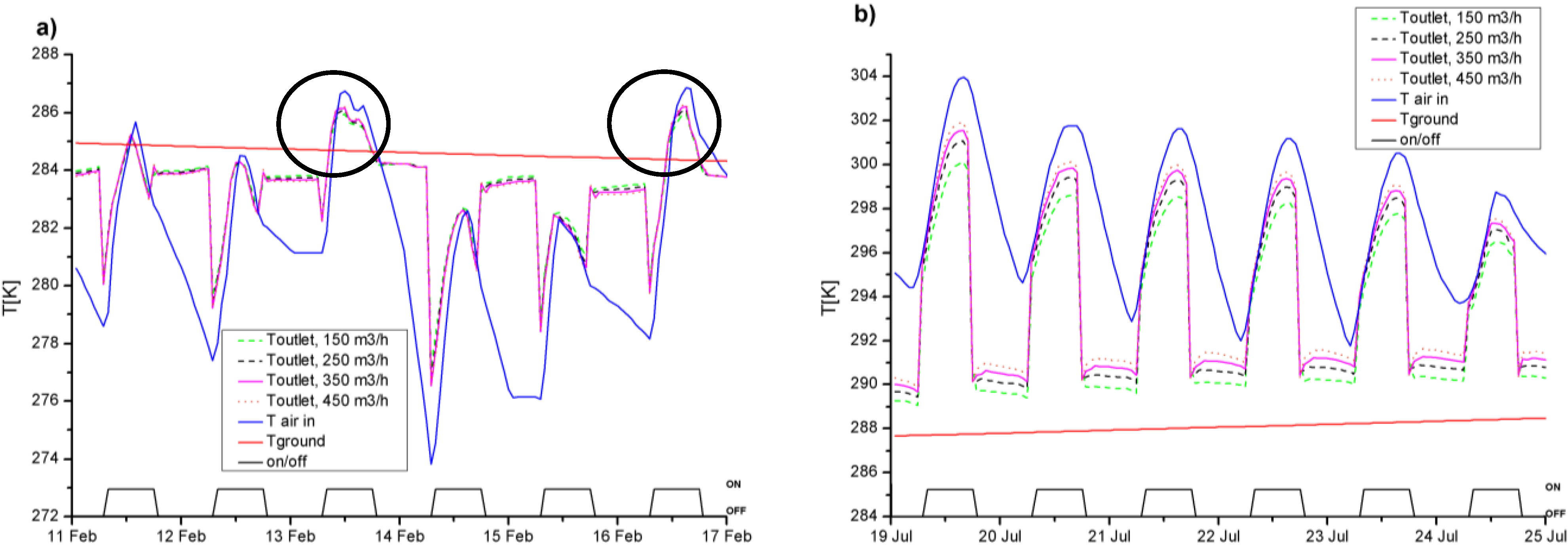
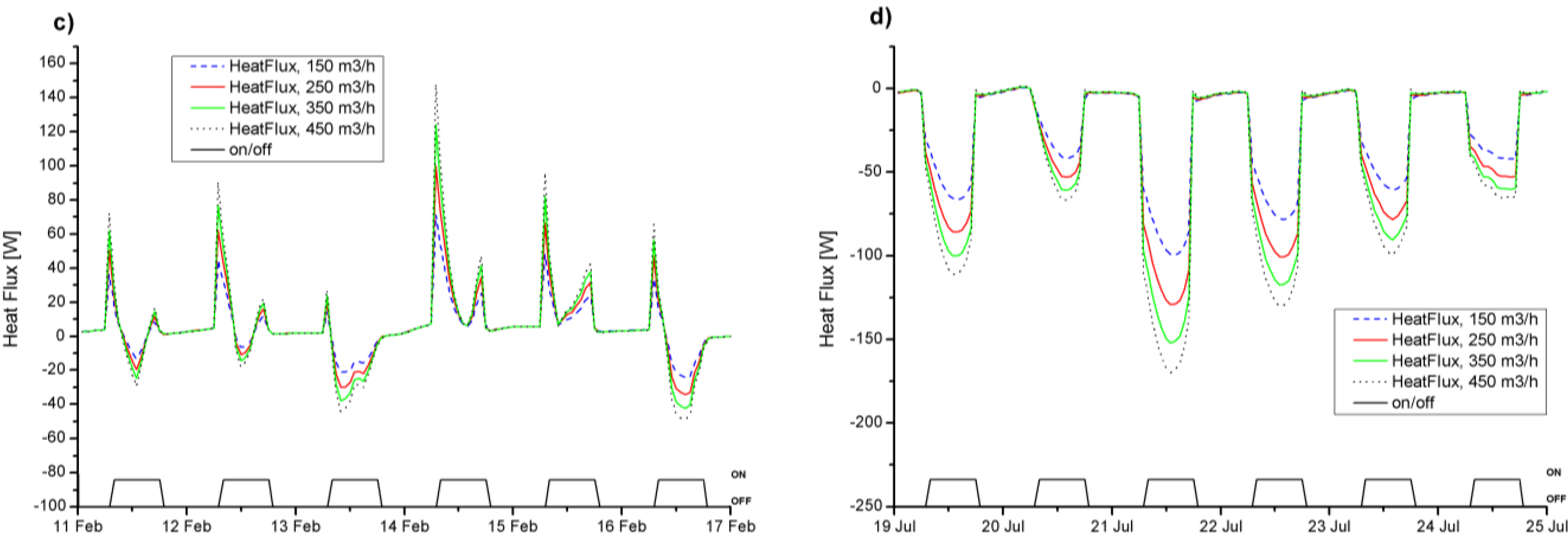
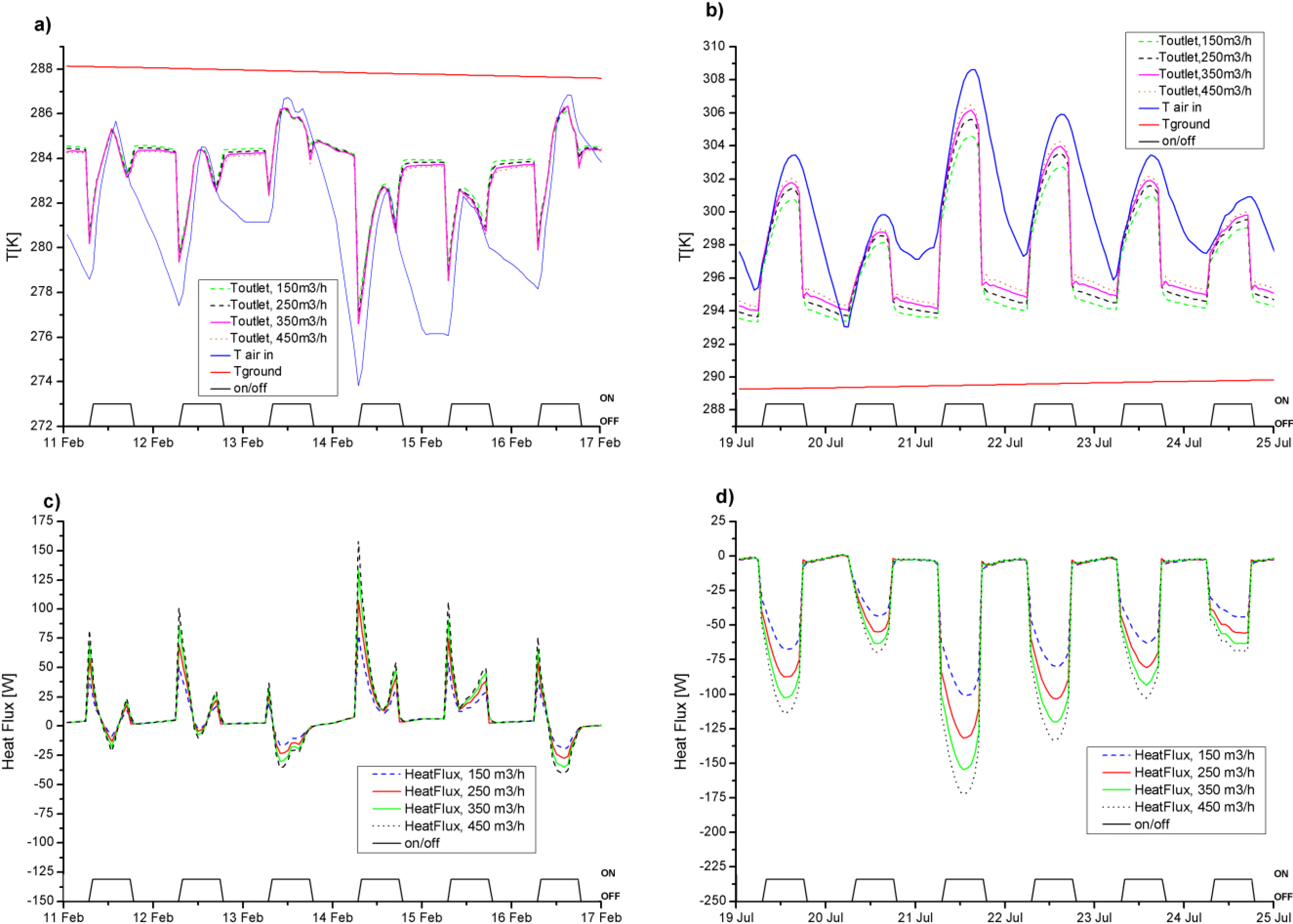
Ground and inlet-outlet air temperatures with λ = 1 W/m K, air-ground thermal power varying the air flow rate (range 150–450 m3 per hour), for typical winter (a,c) and summer weeks (b,d).
Figure 12.
Ground and inlet-outlet air temperatures with λ = 1 W/m K, air-ground thermal power varying the air flow rate (range 150–450 m3 per hour), for typical winter (a,c) and summer weeks (b,d).
Figure 13.
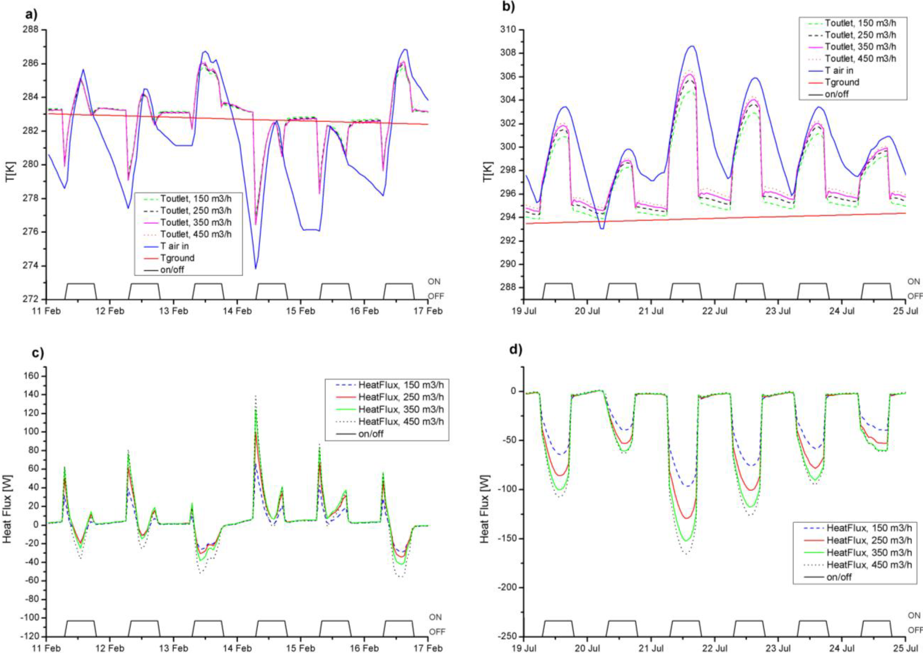
Ground and inlet-outlet air temperatures with λ = 2 W/m K, air-ground thermal power varying the air flow rate (range 150–450 m3 per hour), for typical winter (a,c) and summer weeks (b,d).
Figure 13.
Ground and inlet-outlet air temperatures with λ = 2 W/m K, air-ground thermal power varying the air flow rate (range 150–450 m3 per hour), for typical winter (a,c) and summer weeks (b,d).
Figure 14.
Ground and inlet-outlet air temperatures with λ = 3 W/m K, air-ground thermal power varying the air flow rate (range 150–450 m3 per hour), for typical winter (a,c) and summer weeks (b,d).
Figure 14.
Ground and inlet-outlet air temperatures with λ = 3 W/m K, air-ground thermal power varying the air flow rate (range 150–450 m3 per hour), for typical winter (a,c) and summer weeks (b,d).
The performance results were represented for the weeks in which climatic conditions are more “strict”; for winter, the week with the minimum peak temperature of the year is from 11 to 17 February, in summer, the week with the maximum peak temperature of the year is from 19 to 25 July (year 2002). During both weeks in winter and summer, the outlet air temperature shows, for each daily shutdown of the geothermal plant, an asymptotic behavior at the ground temperature, this henceforth will be called base-line. The value of the base-line depends on the thermal conductivity of the ground; in fact, the base-line tends to overlap the temperature of the ground faster, by increasing thermal conductivity (see
Figure 12a and
Figure 14a).
Figure 15.
Inlet-outlet air temperatures, air-ground thermal power varying the soil conductivity λ = 1–3 W/m K, fixed air flow rate 350 m3/h, for typical winter (a,c) and summer weeks (b,d).
Figure 15.
Inlet-outlet air temperatures, air-ground thermal power varying the soil conductivity λ = 1–3 W/m K, fixed air flow rate 350 m3/h, for typical winter (a,c) and summer weeks (b,d).
The principle that the air is in thermal equilibrium with the ground, during the shutdown of the plant is, certainly, plausible and well managed by the simulation in the CFD code, according to the settings on the back flow. The base line has a correlation, in the diagrams of heat flux, with the value of zero flux. The heat flux is related to the entire pipe and not to semi-pipe. The heat flux is assumed negative, when the air circulating in the duct transfers heat to the ground.
The trends of outlet air temperatures and the corresponding heat fluxes show an unsuitable behavior of the geothermal plant, during the winter. Although 11–17 February is a cold week, the results show the presence of negative peaks in heat transfer, in almost every ON-block. This means that the plant is not able to handle the heating of inlet air, during the whole daily ON-block (the classic office hours). It can happen that, often around 12:00 am, the inlet air temperature “overtakes” the ground temperature, making the reversal of flow (see
Figure 13a).
Instead, the behavior of the HAGHE in summer is significantly positive; with the system switched on, the heat fluxes are always negative in order to pre-cooling the inlet air, depending on the air flow rate.
Figure 12b and
Figure 14b, show a temperature decrease of 0°–4°, according to the air flow rate, with a pipe only 5 m long.
In
Figure 12b, observing the peak relative to the 21 July, can be seen that the air is undisturbed at a temperature of 309 K, while the out of the plant goes from 305 K, for a flow rate of 150 m
3/h, to 307 K, for a flow rate of 450 m
3/h. Clearly, a lower volumetric flow rate input, which means lower air velocity, confer the possibility of a more efficient heat exchange with the ground, for a long probe 5 m; the results are a cooler temperature and a better conditioning, for a flow rate of 150 m
3/h.
Finally,
Figure 15 shows the HAGHE performance by varying the soil conductivity (1, 2, 3 W/m K), keeping constant air flow rate at 350 m
3/h. The first evident difference between winter and summer is that in summer the heat flux is always in the same direction instead in winter the heat flux inversion is possible. Apparently there is a contradiction between
Figure 15a–c because the heat flux grows with the ground thermal conductivity but the outlet air temperature is highest with the lowest value of it. The reason is that ground with lower thermal conductivity is more isolated from the external weather conditions, in winter the ground temperature is higher with lower ground thermal conductivity.
A possible realistic solution to improve the efficiency of HAGHE buried in soil with low thermal conductivity is filling the trench with high thermal conductive materials.
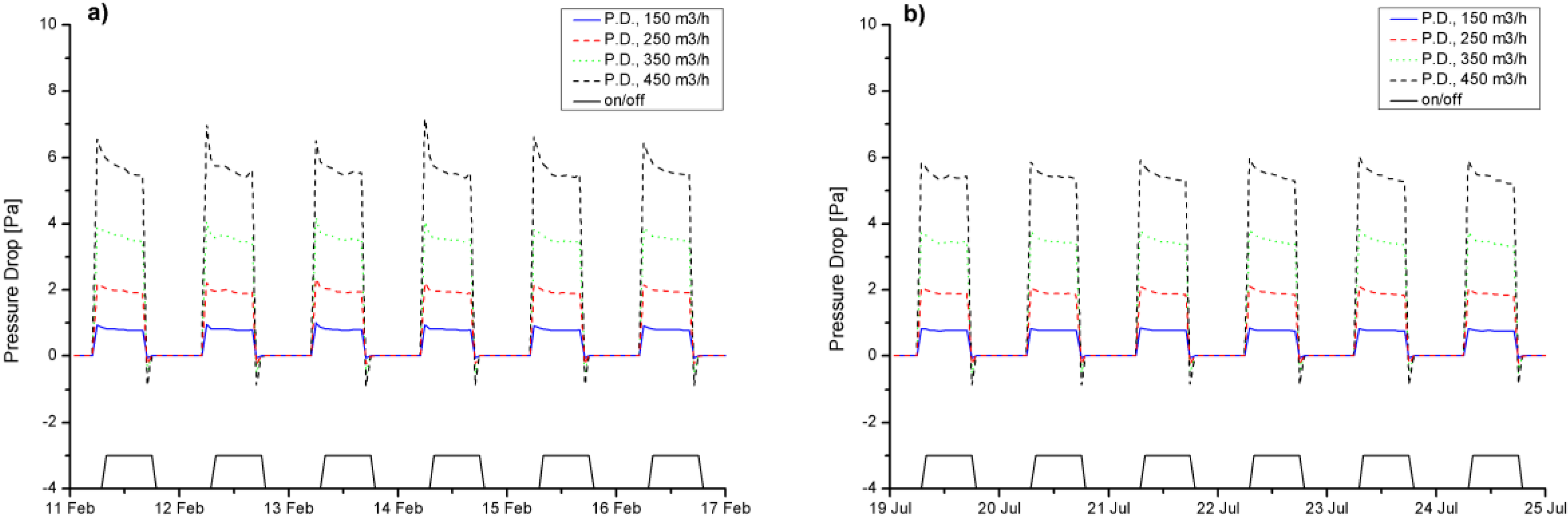
Figure 16a,b show the pressure drops along pipe 5 m long, for winter and summer, respectively.
Concluding the analysis underlines that, in warm climate, during the winter, the HAGHE can be used for a few hours daily and must have a bypass for the external air when the air temperature is higher than one of ground. Instead, during the summer, the HAGHE has huge advantages for cooling the ventilation air. A possible problem should be the relative humidity of air at the end of pipe, therefore it is important to evaluate for each case, if there is a need to keep under control the humidity by a heat pump. In particular, in the historical buildings with moisture dynamics implications [
30,
31], good ventilation using dry air seems to be necessary.
Figure 16.
Pressure drops of air vs. time varying the air mass flow rate for typical: (a) winter week and (b) summer week.
Figure 16.
Pressure drops of air vs. time varying the air mass flow rate for typical: (a) winter week and (b) summer week.
4. Conclusions
This work aims to investigate the performance of HAGHE for HVAC systems. By using the thermal energy stored in the ground, it is possible to pre-heat or pre-cool the ventilation air. HAGHE is a simple superficial system, because the pipes are not buried deep into the ground with air like vector fluid (see
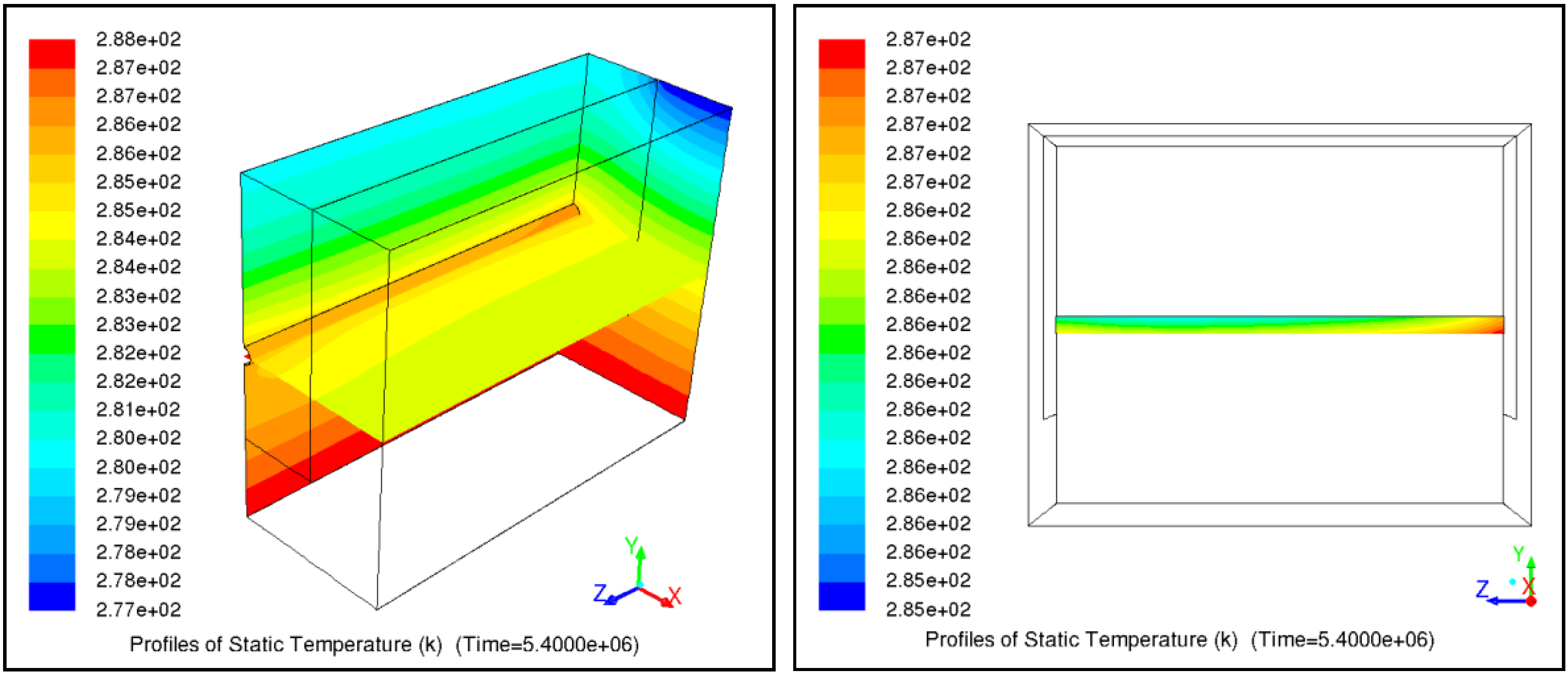
Figure 17). The horizontal geometry of pipes guarantees good heat transfer between air and ground and with a useful stability of air temperature. The horizontal geometry outperforms the vertical configuration, has not the problems related to deep wells, like cost and risk to meet the aquifer.
Figure 17.
Temperature distribution on the horizontal and vertical planes, air flow rate equal to 450 m3/h, with λ = 3 W/(m K), 20 February, at 12 a.m.
Figure 17.
Temperature distribution on the horizontal and vertical planes, air flow rate equal to 450 m3/h, with λ = 3 W/(m K), 20 February, at 12 a.m.
It is interesting to underline that such a condition offers a different strategic possibility, which is the application of HAGHE not for ventilation air but with an air-source heat pump, using the air flux from the HAGHE to keep the behavior of the heat pump stable, reducing the air temperature fluctuations.
The analysis of the results underlines that the HAGHE can be used for a few hours daily with a bypass for the external air when the air temperature is higher than the ground temperature. A smaller volumetric flow rate input, which means lower air velocity, leads to a more efficient heat exchange with the ground, for a 5 m long probe; this results in a cooler temperature and a better conditioning, for a flow rate of 150 m3/h. A comparison at equal flow of air, in function of the conductivity of the soil, shows a slight loss of performance, with the increase of the conductivity value. It is recommended that the heat exchanger be in ground insulation, and consequently less sensitive to thermal changes external; the solution could be a simple conductive trench, limited in size, which surrounds the heat exchanger.
The simulations show significant benefits of HAGH during the summer. The plant is able to process the inlet air during the whole day. The decrease of the outlet air temperature is between 2° and 4°, with a pipe only 5 m long. This offers a good possibility to use the HAGHE for a thermal pre-treatment of ventilation air. Of course the system shows good performance in terms of efficiency and environmental impact if coupled in buildings meeting the n-ZEB or ZEB standards.
Further numerical investigations will be focused on experiments that will be also performed to collect data for a better understanding of the heat transfer phenomenon with the ground, in real operating conditions for a long time.


