System Integration of the Horizontal-Axis Wind Turbine: The Design of Turbine Blades with an Axial-Flux Permanent Magnet Generator


Abstract
:1. Introduction

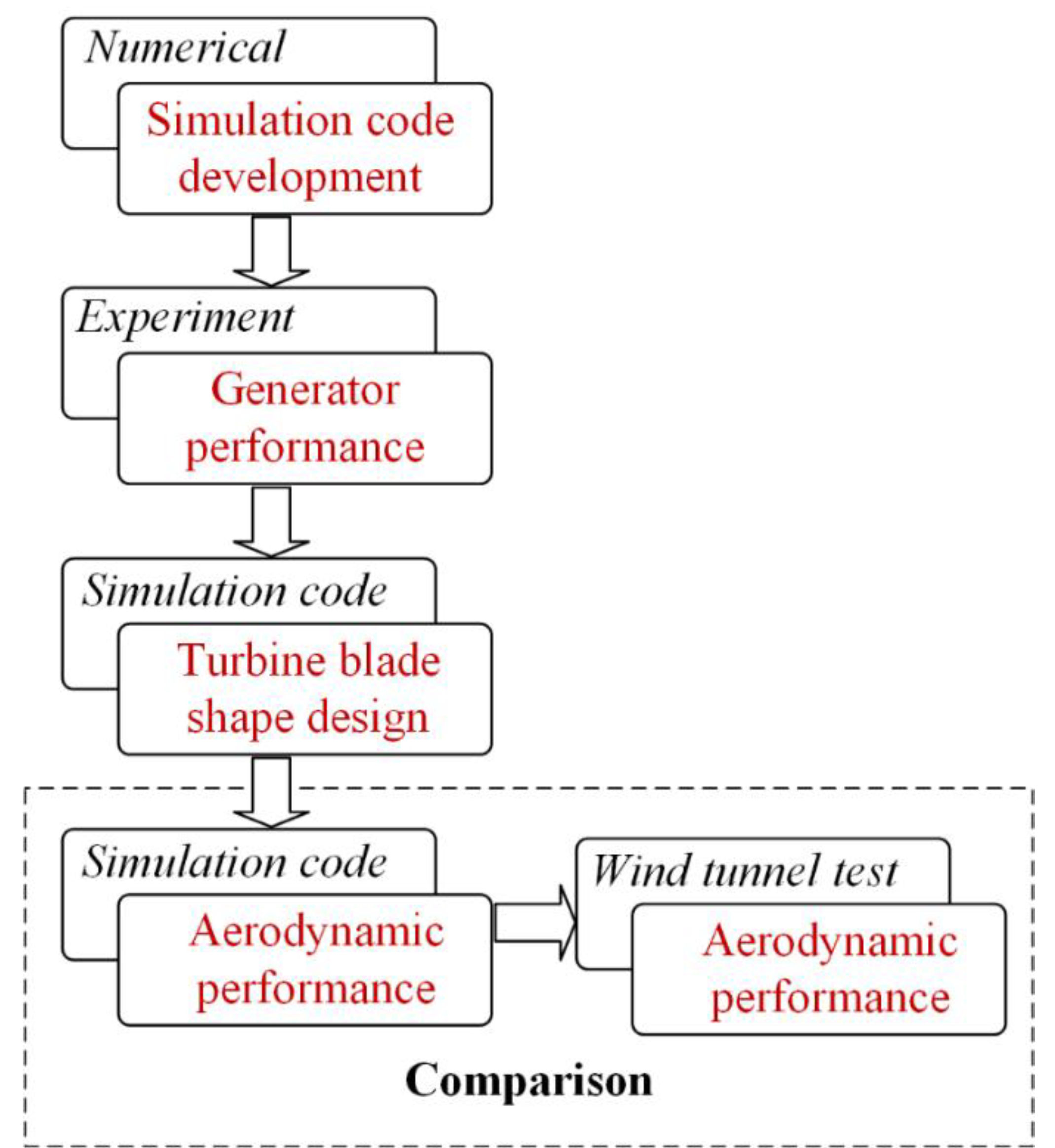
2. Simulation Code

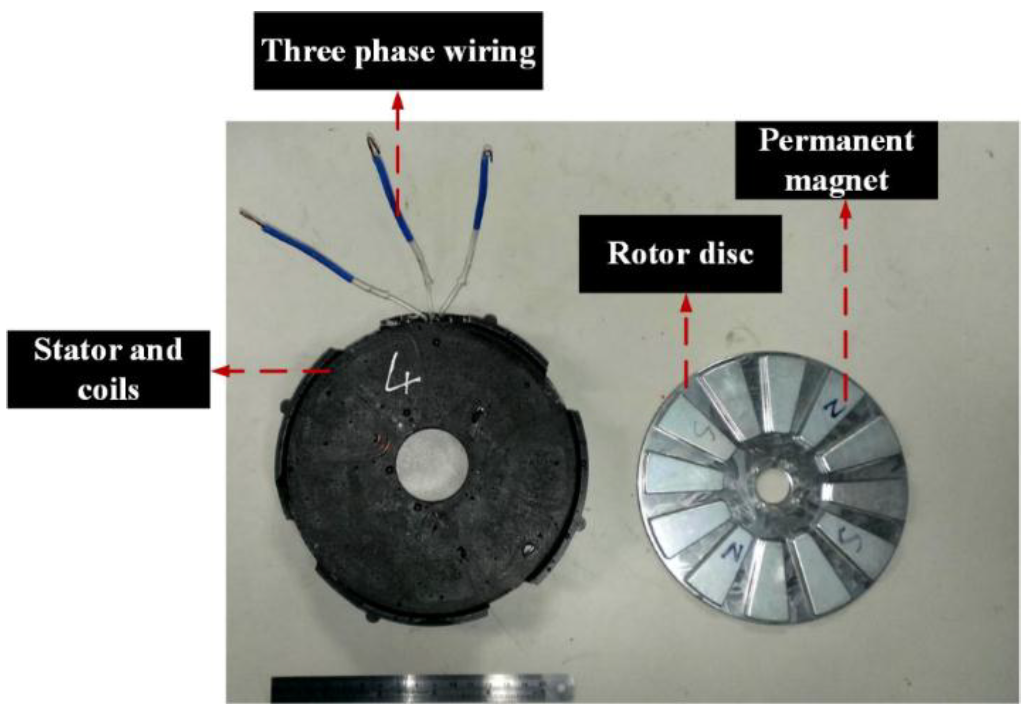
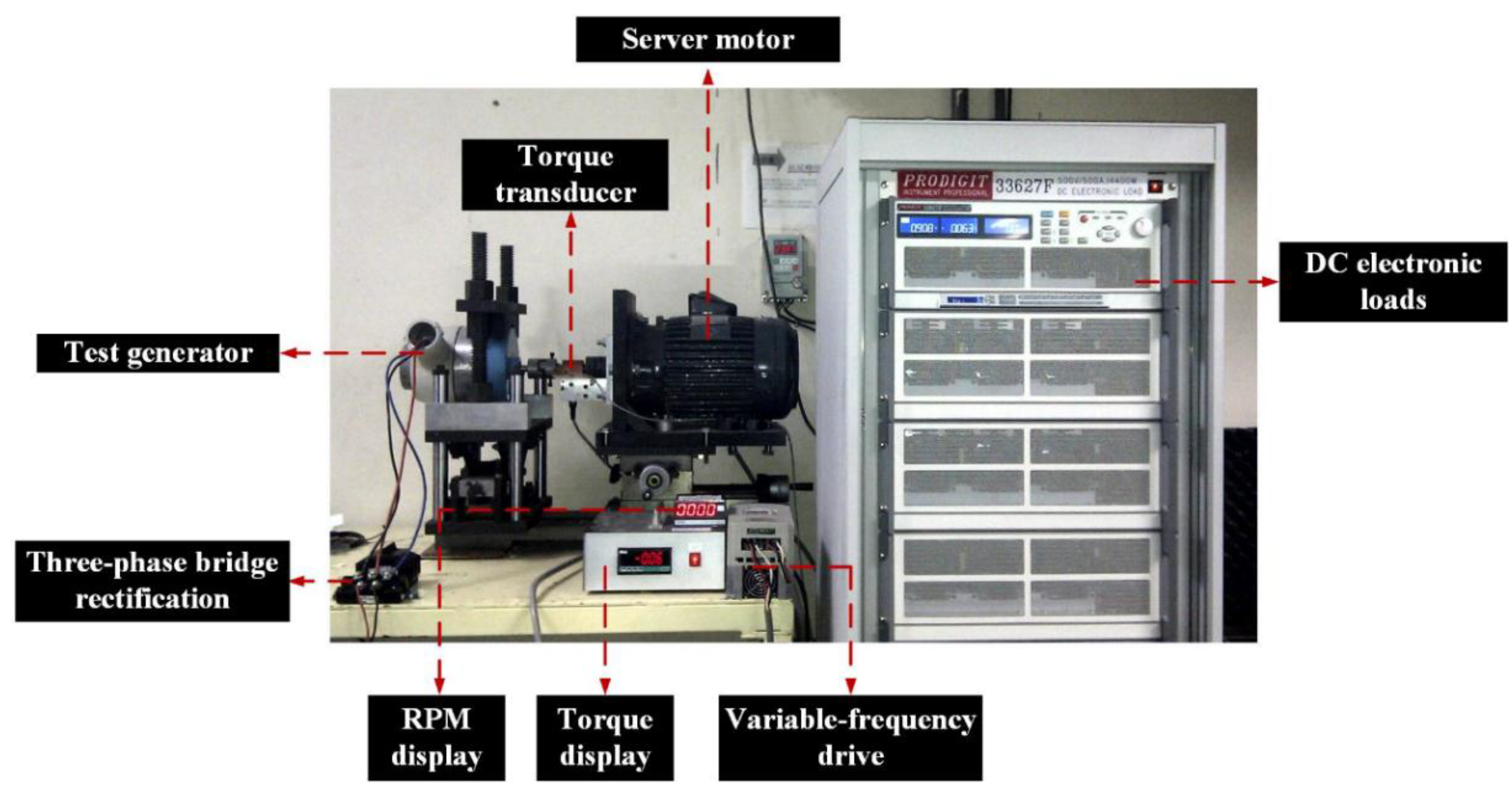
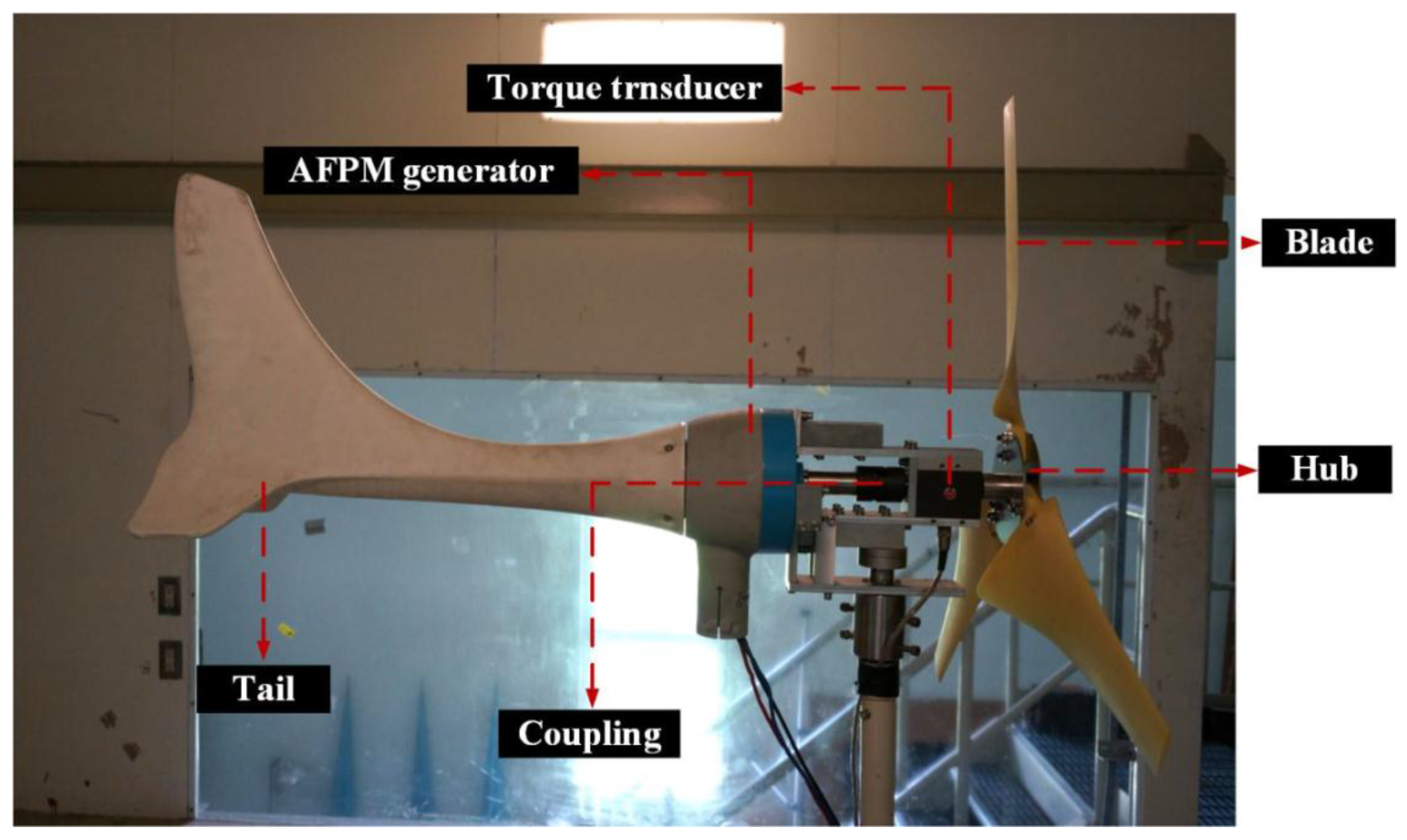
3. The AFPM Generator Test Platform


4. Design of Turbine Blade
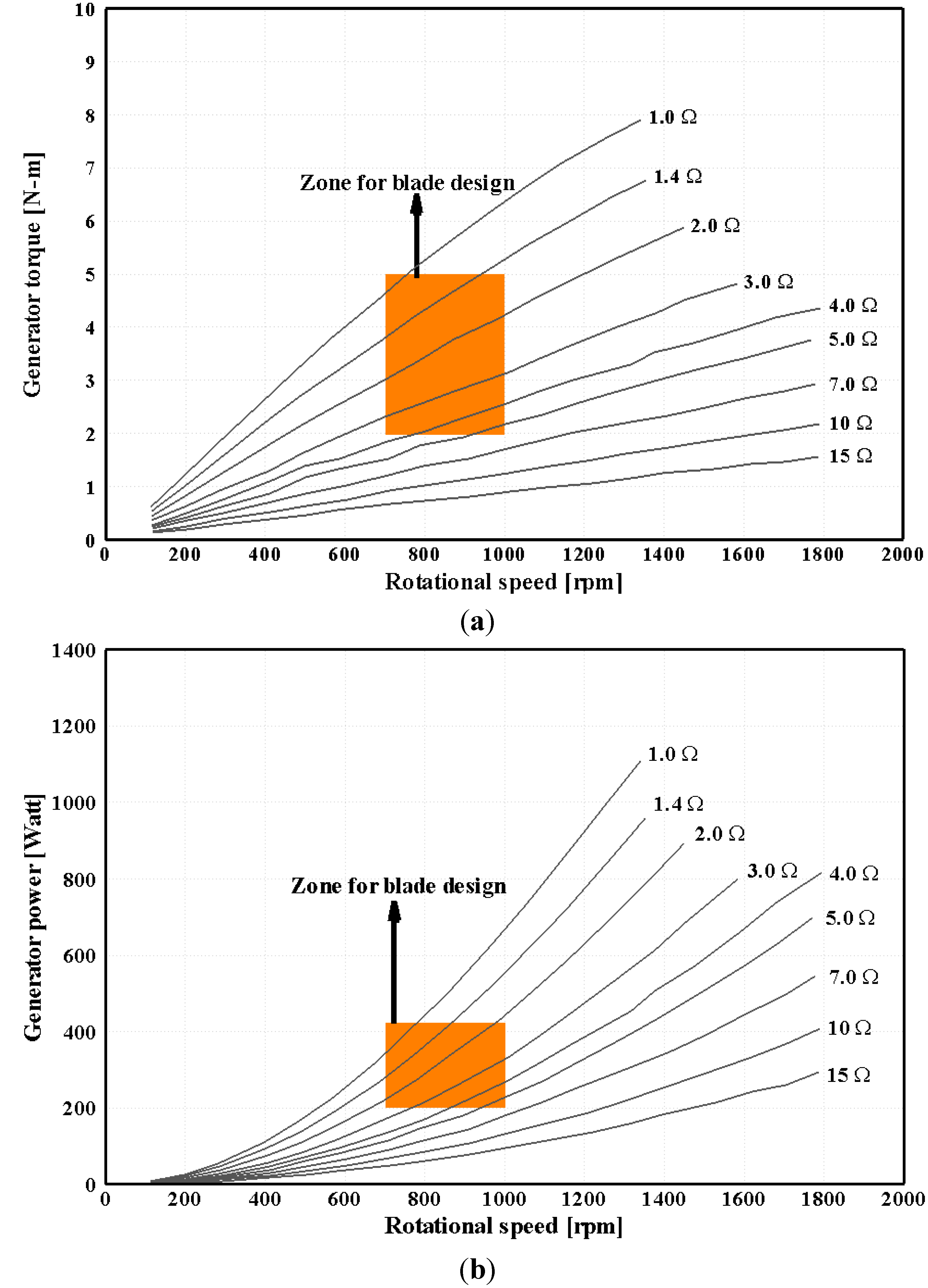
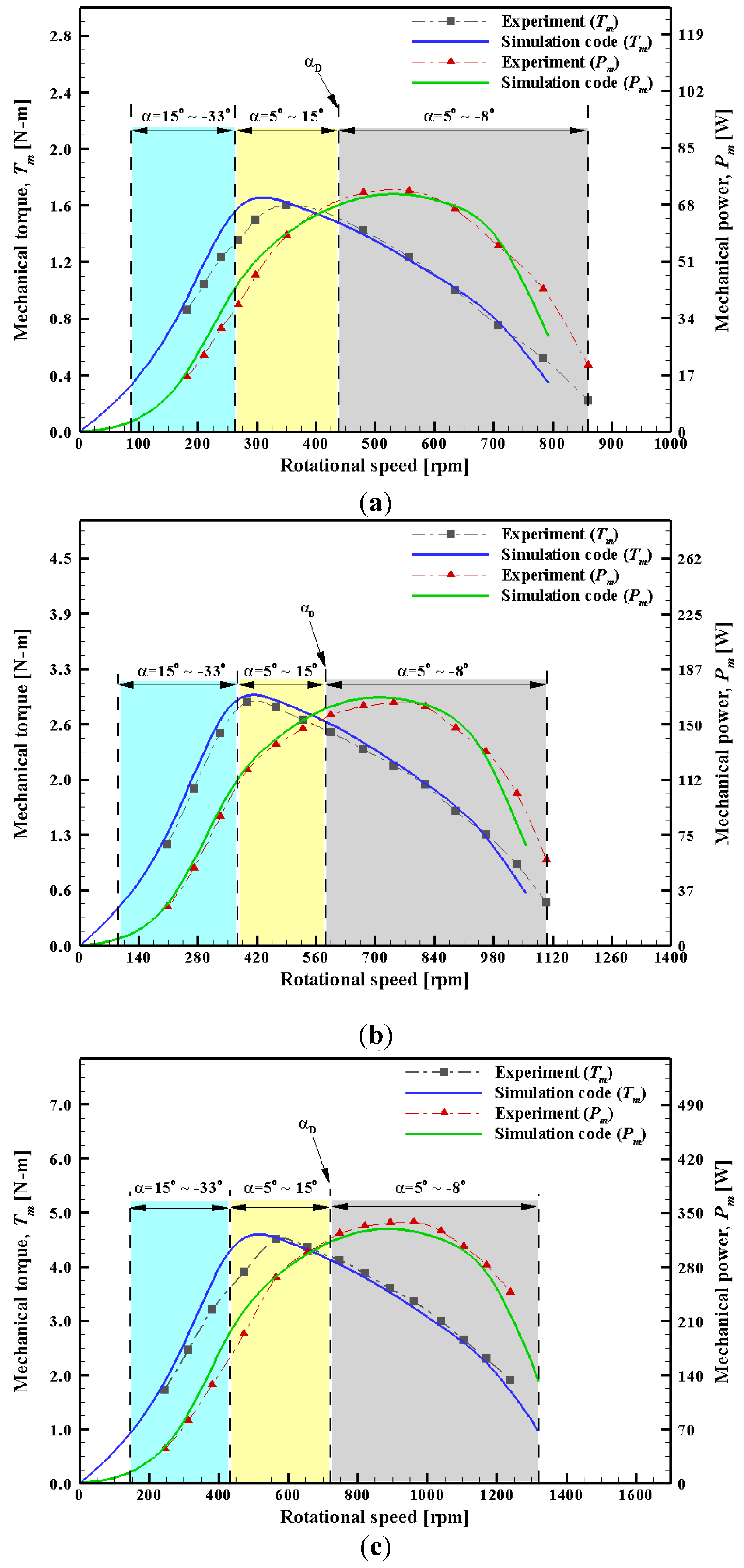
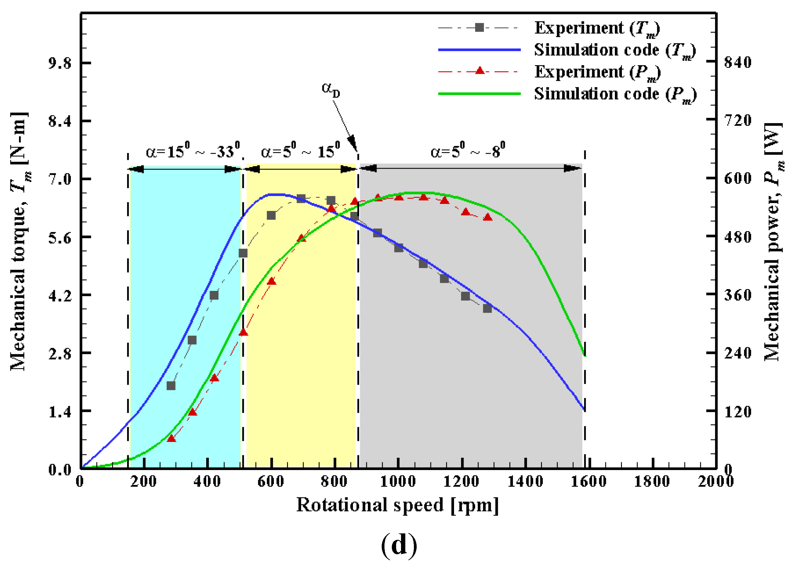
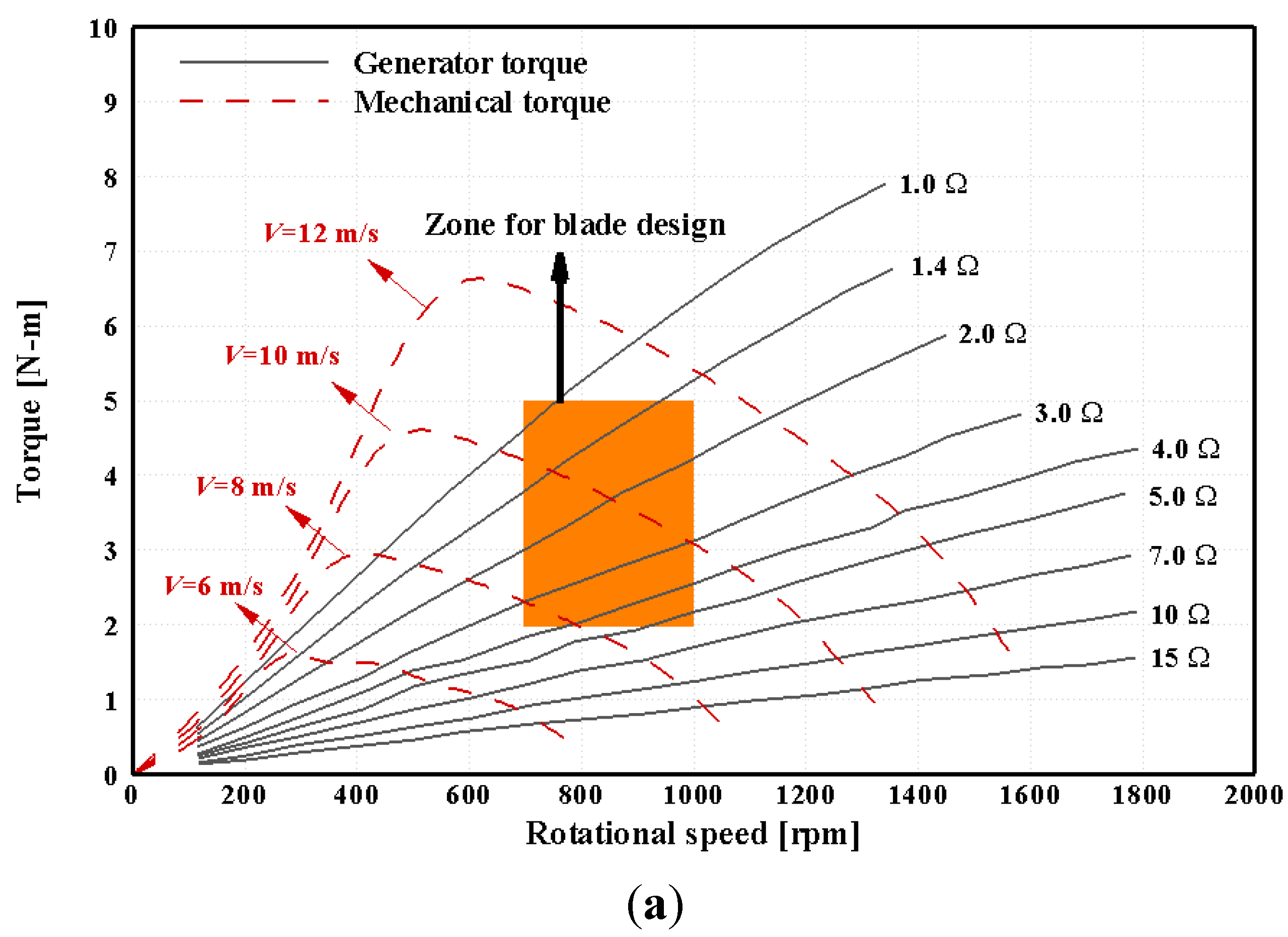
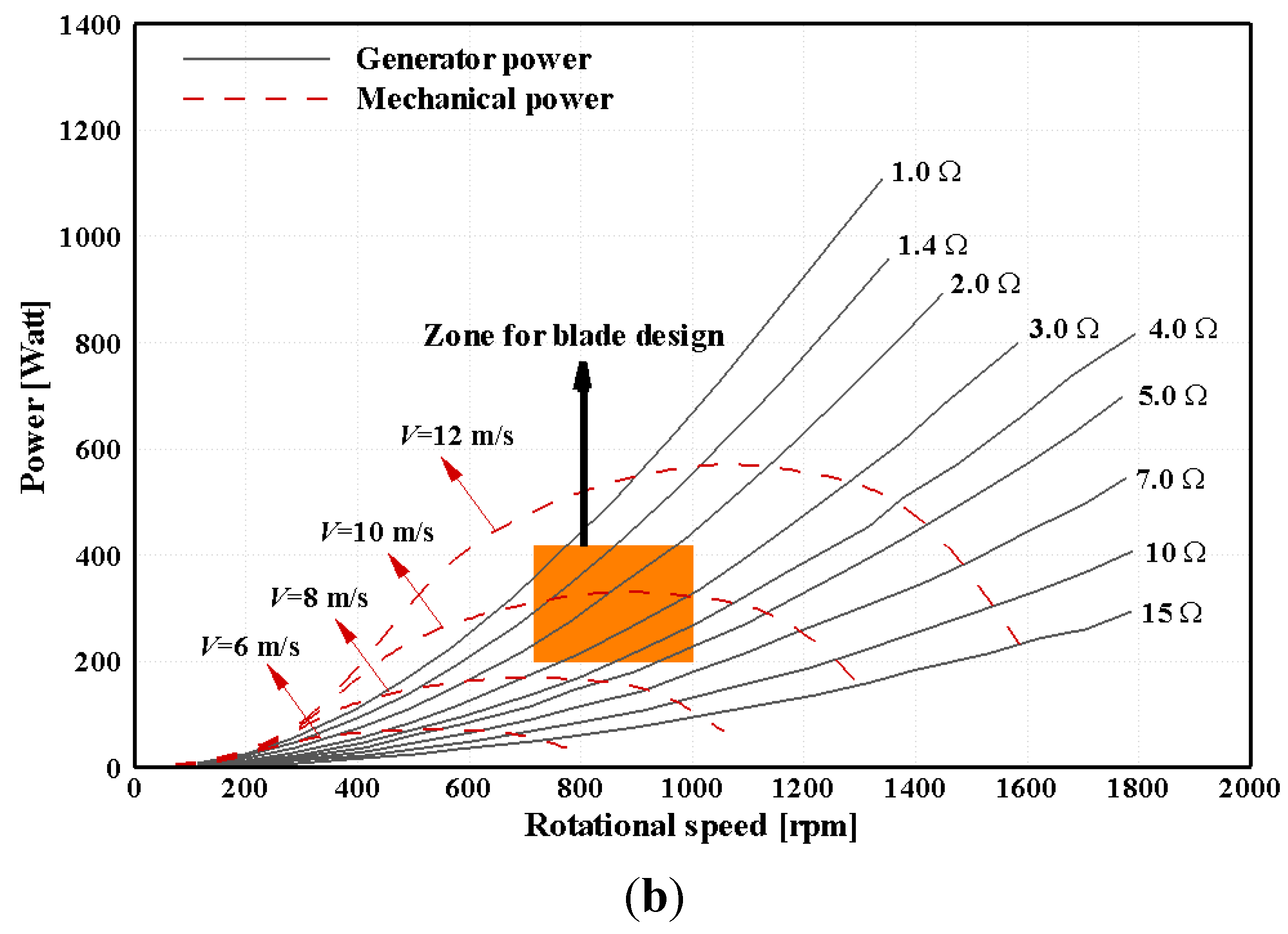
4.1. Performance of AFPM Generator


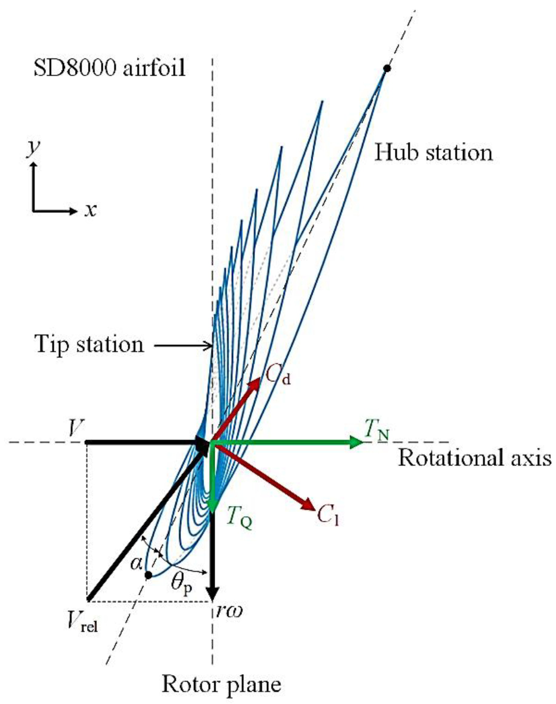
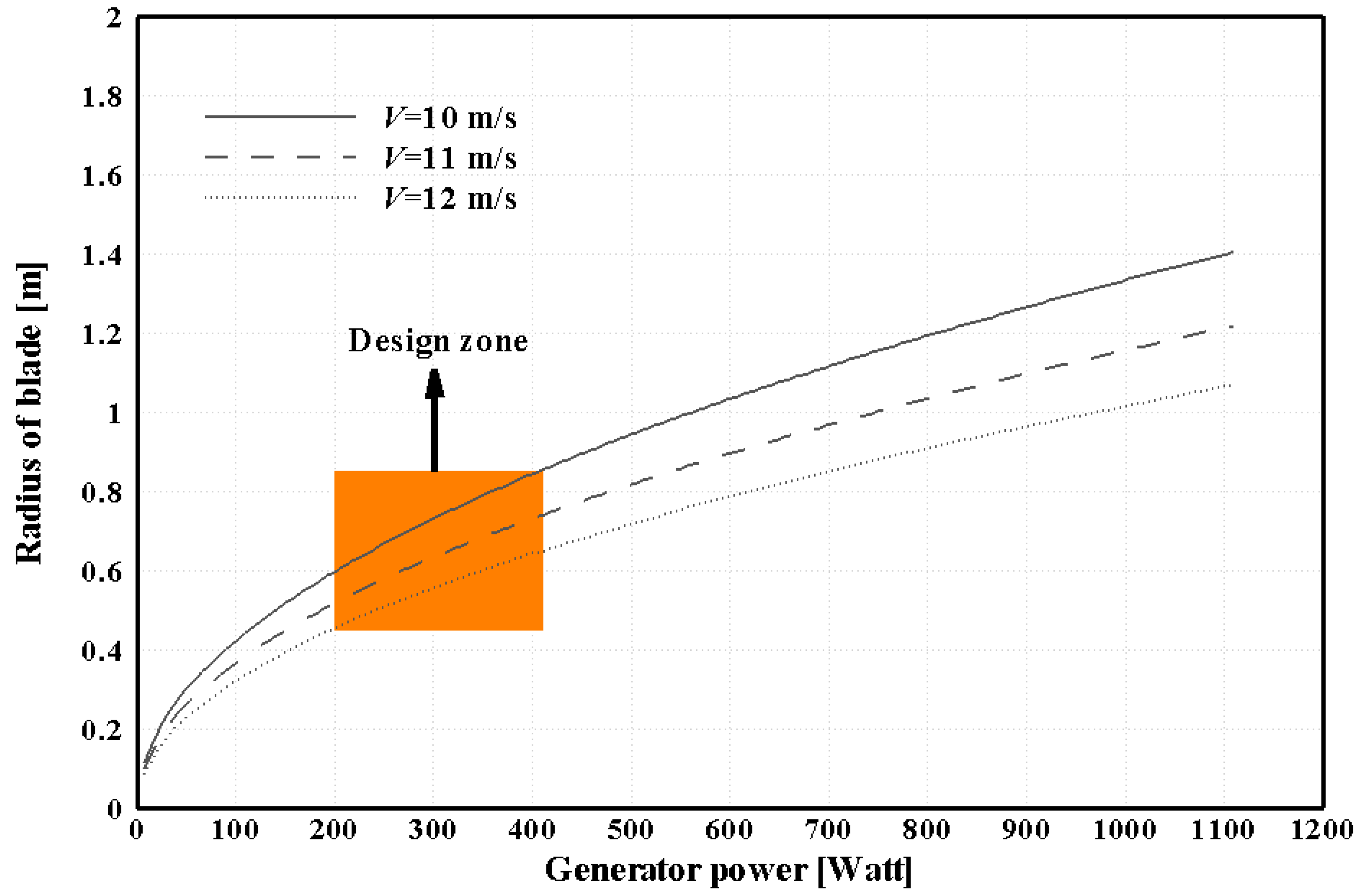
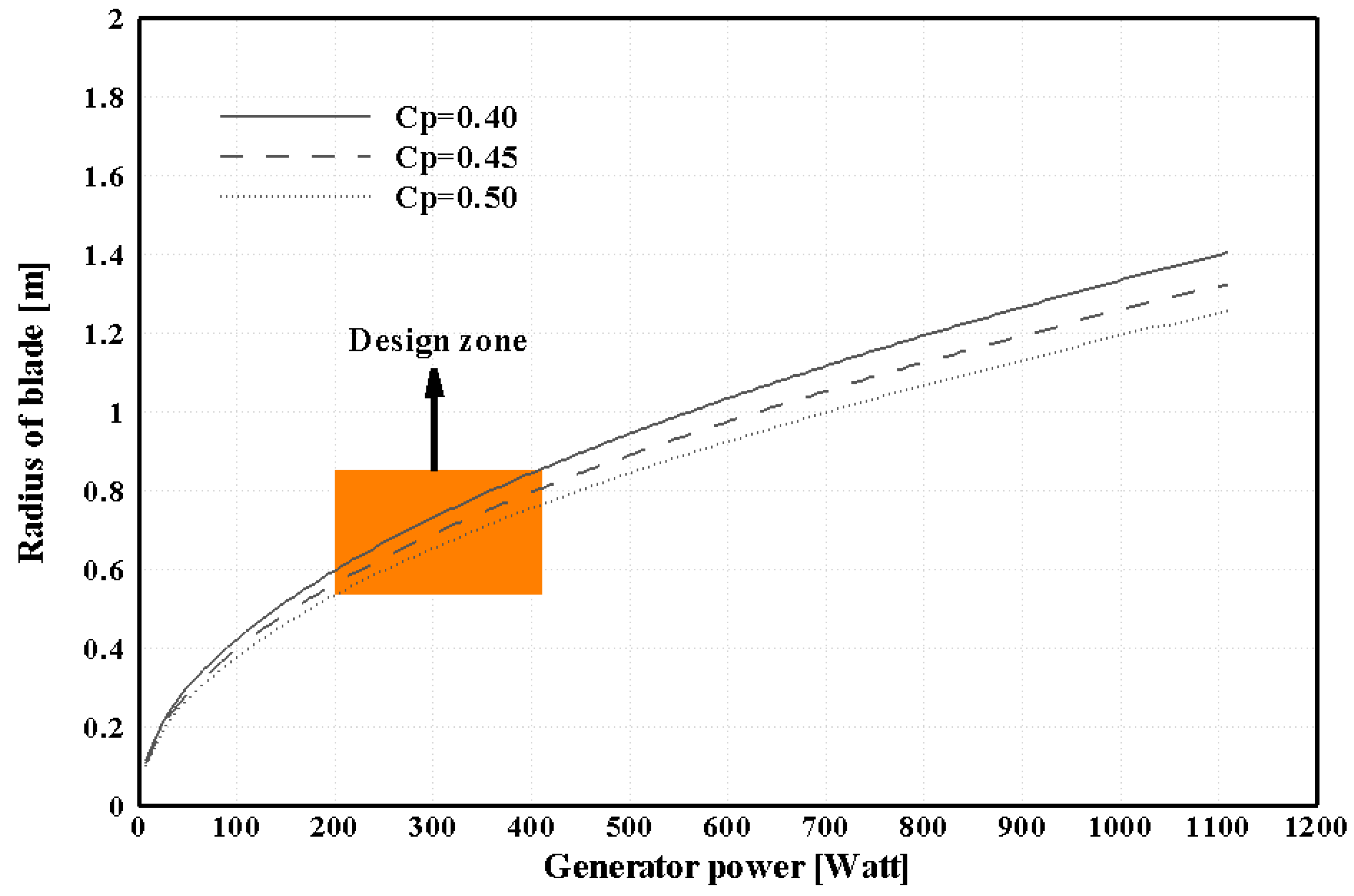
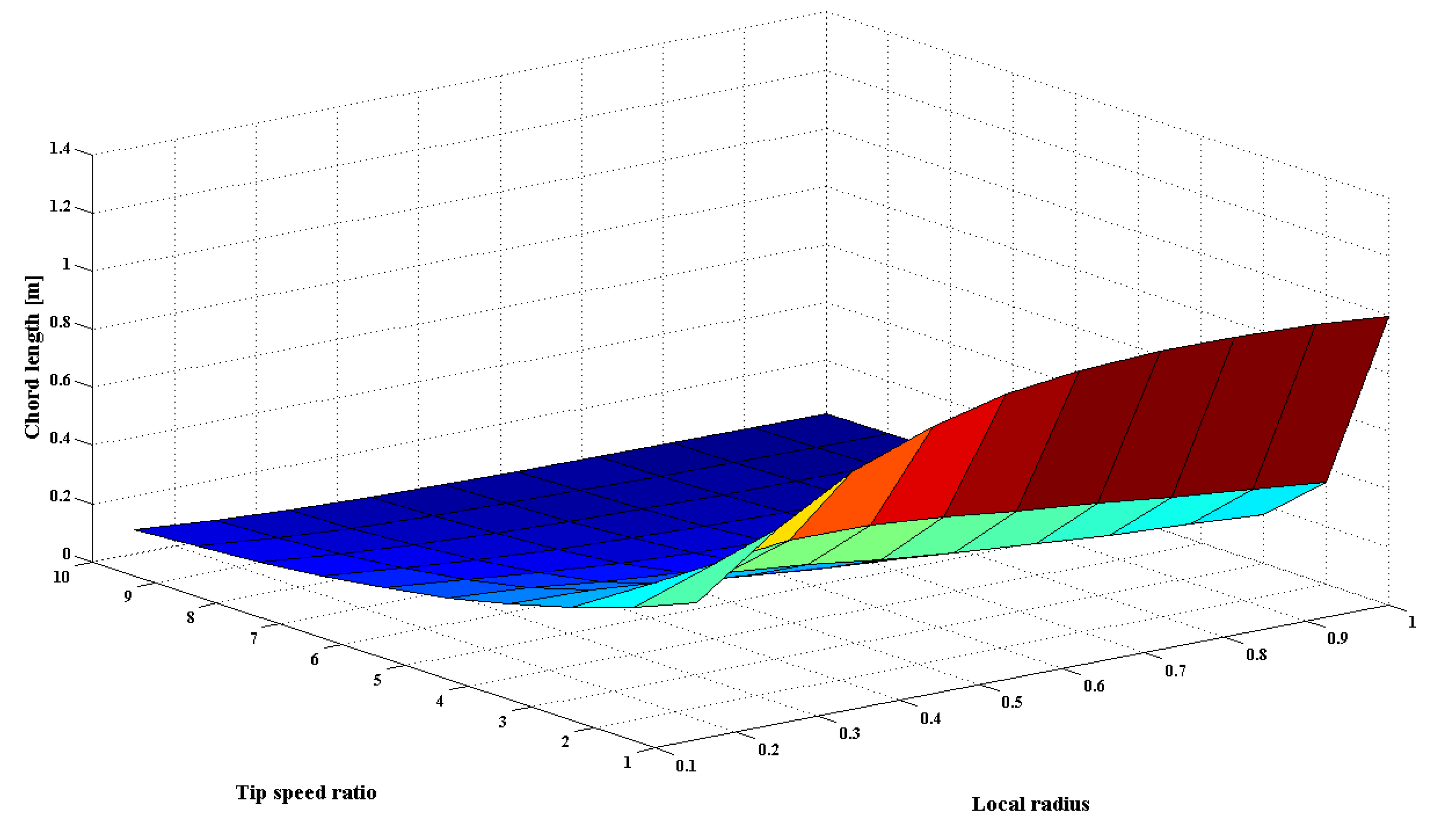
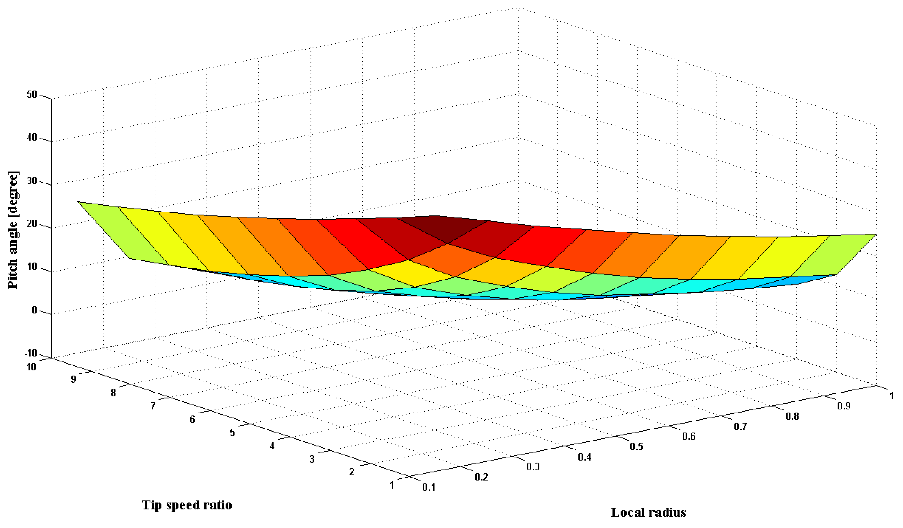
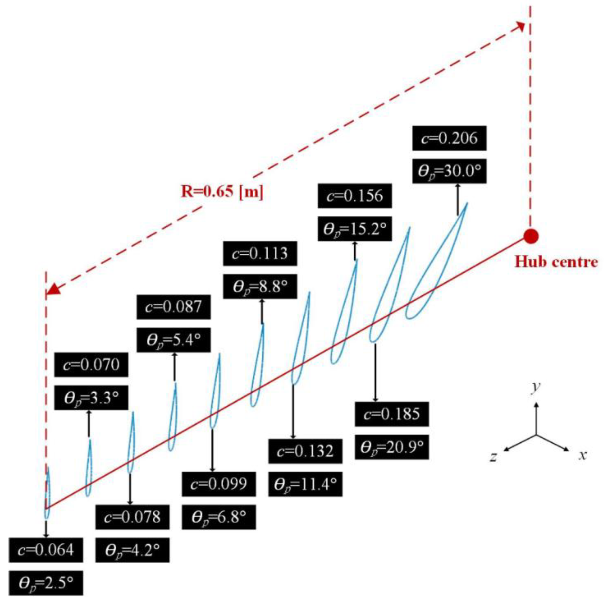
4.2. Geometry for Turbine Blade


| Characteristics | Values |
|---|---|
| Rated power (W) | 400 |
| Rated wind speed (m/s) | 12 |
| Designed tip speed ratio | 5 |
| Number of blades | 3 |
| Designed angle of attack (°) | 5 |
| Airfoil type | SD8000 |

5. Wind Tunnel Testing

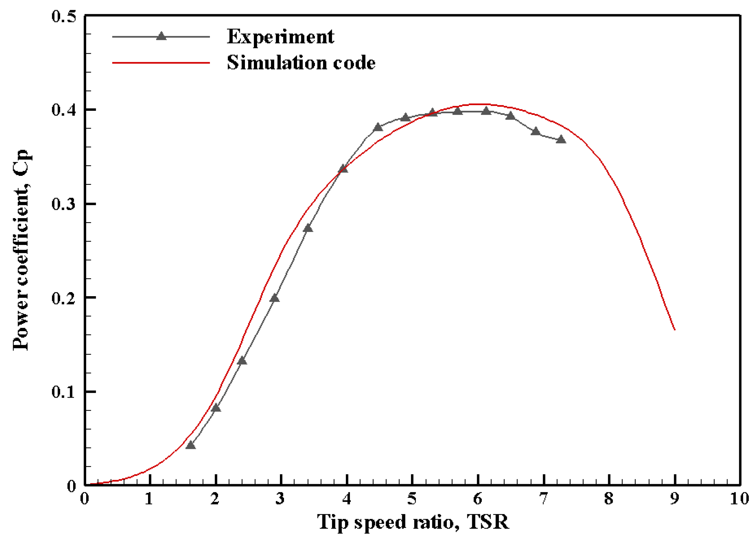
6. Comparison of the Simulation and Experimental Results


7. Conclusions
Acknowledgments
Author Contributions
Conflicts of Interest
References
- Madlener, R.; Latz, J. Economics of centralized and decentralized compressed air energy storage for enhanced grid integration of wind power. Appl. Energy 2013, 101, 299–309. [Google Scholar] [CrossRef]
- McKenna, R.; Hollnaicher, S.; Fichtner, W. Cost-potential curves for onshore wind energy: A high-resolution analysis for Germany. Appl. Energy 2014, 115, 103–115. [Google Scholar] [CrossRef]
- Yang, H.; Wei, Z.; Chengzhi, L. Optimal design and techno-economic analysis of a hybrid solar–wind power generation system. Appl. Energy 2009, 86, 163–169. [Google Scholar] [CrossRef]
- Goundar, J.N.; Ahmed, M.R. Design of a horizontal axis tidal current turbine. Appl. Energy 2013, 111, 161–174. [Google Scholar] [CrossRef]
- Hsiao, F.-B.; Bai, C.-J.; Chong, W.-T. The performance test of three different horizontal axis wind turbine (HAWT) blade shapes using experimental and numerical methods. Energies 2013, 6, 2784–2803. [Google Scholar]
- Lee, J.H.; Park, S.; Kim, D.H.; Rhee, S.H.; Kim, M.-C. Computational methods for performance analysis of horizontal axis tidal stream turbines. Appl. Energy 2012, 98, 512–523. [Google Scholar] [CrossRef]
- Krogstad, P.A.; Lund, J.A. An experimental and numerical study of the perofrmance of a model turbine. WInd Energy 2012, 15, 443–457. [Google Scholar]
- Martínez, J.; Bernabini, L.; Probst, O.; Rodríguez, C. An improved BEM model for the power curve prediction of stall-regulated wind turbines. Wind Energy 2005, 8, 385–402. [Google Scholar] [CrossRef]
- Lanzafame, R.; Messina, M. Fluid dynamics wind turbine design: Critical analysis, optimization and application of BEM theory. Renew. Energy 2007, 32, 2291–2305. [Google Scholar] [CrossRef]
- Dai, J.C.; Hu, Y.P.; Liu, D.S.; Long, X. Aerodynamic loads calculation and analysis for large scale wind turbine based on combining BEM modified theory with dynamic stall model. Renew. Energy 2011, 36, 1095–1104. [Google Scholar] [CrossRef]
- Hirahara, H.; Hossain, M.Z.; Kawahashi, M.; Nonomura, Y. Testing basic performance of a very small wind turbine designed for multi-purposes. Renew. Energy 2005, 30, 1279–1297. [Google Scholar] [CrossRef]
- Kishinami, K.; Taniguchi, H.; Suzuki, J.; Ibano, H.; Kazunou, T.; Turuhami, M. Theoretical and experimental study on the aerodynamic characteristics of a horizontal axis wind turbine. Energy 2005, 30, 2089–2100. [Google Scholar] [CrossRef]
- Bottasso, C.L.; Campagnolo, F.; Petrović, V. Wind tunnel testing of scaled wind turbine models: Beyond aerodynamics. J. Wind Eng. Ind. Aerodyn. 2014, 127, 11–28. [Google Scholar] [CrossRef]
- Sheng, W.; Galbraith, R.A.M.; Coton, F.N. On the S809 airfoil’s unsteady aerodynamic characteristics. Wind Energy 2009, 12, 752–767. [Google Scholar] [CrossRef]
- Vermeer, L.J.; Sørensen, J.N.; Crespo, A. Wind turbine wake aerodynamics. Progr. Aerosp. Sci. 2003, 39, 467–510. [Google Scholar] [CrossRef]
- Hansen, A.D.; Sørensen, P.; Iov, F.; Blaabjerg, F. Control of variable speed wind turbines with DFIGs. Wind Eng. 2004, 28, 411–434. [Google Scholar] [CrossRef]
- Lei, Y.; Mullane, A.; Lightbody, G.; Yacamini, R. Modeling of the wind turbine with a doubly fed induction generator for grid integration studies. IEEE Tran. Energy Convers. 2006, 21, 257–264. [Google Scholar] [CrossRef]
- González, L.G.; Figueres, E.; Garcerá, G.; Carranza, O. Maximum-power-point tracking with reduced mechanical stress applied to wind-energy-conversion-systems. Appl. Energy 2010, 87, 2304–2312. [Google Scholar] [CrossRef]
- Carranza, O.; Figueres, E.; Garcerá, G.; Gonzalez-Medina, R. Analysis of the control structure of wind energy generation systems based on a permanent magnet synchronous generator. Appl. Energy 2013, 103, 522–538. [Google Scholar] [CrossRef]
- Arroyo, A.; Manana, M.; Gomez, C.; Fernandez, I.; Delgado, F.; Zobaa, A.F. A methodology for the low-cost optimisation of small wind turbine performance. Appl. Energy 2013, 104, 1–9. [Google Scholar] [CrossRef]
- Amrouche, B.; Guessoum, A.; Belhamel, M. A simple behavioural model for solar module electric characteristics based on the first order system step response for MPPT study and comparison. Appl. Energy 2012, 91, 395–404. [Google Scholar] [CrossRef]
- Brahmi, J.; Krichen, L.; Ouali, A. A comparative study between three sensorless control strategies for PMSG in wind energy conversion system. Appl. Energy 2009, 86, 1565–1573. [Google Scholar] [CrossRef]
- Song, Z.; Xia, C.; Shi, T. Assessing transient response of DFIG based wind turbines during voltage dips regarding main flux saturation and rotor deep-bar effect. Appl. Energy 2010, 87, 3283–3293. [Google Scholar] [CrossRef]
- Rahimi, M.; Parniani, M. Grid-fault ride-through analysis and control of wind turbines with doubly fed induction generators. Electr. Power Syst. Res. 2010, 80, 184–195. [Google Scholar] [CrossRef]
- Mahmoudi, A.; Rahim, N.A.; Ping, H.W. Axial-flux permanent-magnet motor design for electric vehicle direct drive using sizing equation and finite element analysis. Prog. Electromagn. Res. 2012, 122, 467–496. [Google Scholar] [CrossRef]
- Jung, T.-U. Electromagnetic design analysis and performance improvement of axial field permanent magnet generator for small wind turbine. J. Appl. Phys. 2012, 111, 07E708. [Google Scholar]
- Manwell, J.F.; McGowan, J.G.; Rogers, A.L. Wind Energy Explained-Theory, Design and Application, 2nd ed.; John Wiley & Sons Ltd.: Chichester, West Sussex, UK, 2010. [Google Scholar]
- Barlow, J.B.; Rae, W.H., Jr.; POPE, A. Low-Speed Wind Tunnel Testing, 3rd ed.; Wiley-Interscience: New York, NY, USA, 1999. [Google Scholar]
- Viterna, L.A.; Corrigan, R.D. Fixed pitch rotor performance of large horizontal axis wind turbines. In Proceedings of the DOE/NASA Workshop on Large Horizontal Axis Wind Turbine, Cleveland, OH, USA, 28–30 July 1981; Volume 15, pp. 69–85.
- Chan, T.F.; Lai, L.L. An Axial-flux permanent-magnet synchronous generator for a direct-coupled wind-turbine system. IEEE Trans. Energy Convers. 2007, 22, 86–94. [Google Scholar] [CrossRef]
- Spera, D.A. Wind Turbine Technology: Fundamental Concepts of Wind Turbine Engineering; ASME Press: New York, NY, USA, 1994. [Google Scholar]
- Chen, T.Y.; Liou, L.R. Blockage corrections in wind tunnel tests of small horizontal-axis wind turbines. Exp. Therm. Fluid Sci. 2011, 35, 565–569. [Google Scholar] [CrossRef]
- Simms, D.; Schreck, S.; Hand, M.; Fingersh, L.J. NREL Unsteady Aerodynamics Experiment in the NASA-Ames Wind Tunnel: Comparison of Predictions to Measurements; BiblioGov: Golden, CO, USA, 2001. [Google Scholar]
© 2014 by the authors; licensee MDPI, Basel, Switzerland. This article is an open access article distributed under the terms and conditions of the Creative Commons Attribution license (http://creativecommons.org/licenses/by/4.0/).
Share and Cite
Bai, C.-J.; Wang, W.-C.; Chen, P.-W.; Chong, W.-T. System Integration of the Horizontal-Axis Wind Turbine: The Design of Turbine Blades with an Axial-Flux Permanent Magnet Generator. Energies 2014, 7, 7773-7793. https://doi.org/10.3390/en7117773
Bai C-J, Wang W-C, Chen P-W, Chong W-T. System Integration of the Horizontal-Axis Wind Turbine: The Design of Turbine Blades with an Axial-Flux Permanent Magnet Generator. Energies. 2014; 7(11):7773-7793. https://doi.org/10.3390/en7117773
Chicago/Turabian StyleBai, Chi-Jeng, Wei-Cheng Wang, Po-Wei Chen, and Wen-Tong Chong. 2014. "System Integration of the Horizontal-Axis Wind Turbine: The Design of Turbine Blades with an Axial-Flux Permanent Magnet Generator" Energies 7, no. 11: 7773-7793. https://doi.org/10.3390/en7117773
APA StyleBai, C.-J., Wang, W.-C., Chen, P.-W., & Chong, W.-T. (2014). System Integration of the Horizontal-Axis Wind Turbine: The Design of Turbine Blades with an Axial-Flux Permanent Magnet Generator. Energies, 7(11), 7773-7793. https://doi.org/10.3390/en7117773