Game-Theoretic Energy Management for Residential Users with Dischargeable Plug-in Electric Vehicles

Abstract

The plug-in electric vehicle (PEV) has attracted more and more attention because of the energy crisis and environmental pollution, which is also the main shiftable load of the residential users’ demand side management (DSM) system in the future smart grid (SG). In this paper, we employ game theory to provide an autonomous energy management system among residential users considering selling energy back to the utility company by discharging the PEV’s battery. By assuming all users are equipped with smart meters to execute automatic energy consumption scheduling (ECS) and the energy company can adopt adequate pricing tariffs relating to time and level of energy usage, we formulate an energy management game, where the players are the residential users and the strategies are their daily schedules of household appliance use. We will show that the Nash equilibrium of the formulated energy management game can guarantee the global optimization in terms of minimizing the energy costs, where the depreciation cost of PEV’s battery because of discharging and selling energy back is also considered. Simulation results verify that the proposed game-theoretic approach can reduce the total energy cost and individual daily electricity payment. Moreover, since plug-in electric bicycles (PEBs) are currently widely used in China, simulation results of residential users owing household appliances and bidirectional energy trading of PEBs are also provided and discussed.

1. Introduction

As the operation of electric energy systems, the classic unidirectional top-down oriented power grid has gradually been transformed and upgraded to the two-way smart grid (SG). Physical implementations of SG integration, such as the MeRegioMobil project in Karlsruhe, Germany [1,2], which can realize bi-directional power flows between vehicles and a smart home, are already in place. A strong driver for SG approaches is to integrate fluctuating renewable energy (wind and solar) into the power grid. In order to smooth the fluctuations of the distributed renewable energy generations, energy storage and demand side management (DSM) are widely considered in SG. For electrical energy storage, chemical energy carriers have been widely used currently, such as different types of batteries equipped in plug-in electric vehicles (PEVs) [3], although they are still subjected to the range anxiety [2]. DSM generally refers to such activities implemented to improve energy efficiency and reduce cost at the customer side and control the energy consumption [4]. It is also designed to reduce peak-to-average ratio (PAR) and balance power supply and demand [5]. Another advantage of DSM is that it is less expensive to intelligently influence a load than to build a new power plant or install energy storage devices [6]. Although the main users of DSM consist of residential users, commercial users, and industrial users, optimizing residential energy consumption has emerged as a hot topic [7] because of the large number of residential customers, and we are almost ready with the developed and developing technologies related to SG, especially equipped household smart meters [8].

The main categories of DSM for residential users are energy efficiency, smart pricing, and direct load control (DLC). Energy efficiency methods include all permanent changes to equipment or improvements to the physical properties of the system, which will result in immediate and permanent energy and emissions savings and is therefore the most welcome method [6]. Further, the drawback of energy efficiency is that the one time investment is expensive. In DLC programs, the utility company can remotely control the operations of certain household appliances based on an agreement between the utility company and the customers. The major concern of DLC would be users’ privacy, which will be a barrier in the real implementation for residential users [9]. Smart pricing, including critical-peak pricing [10], time-of-use (ToU) pricing, and real-time pricing [11], has attracted growing attention, both in academia and industry, which means the utility company uses time-dependent electric prices to encourage customers to schedule their shiftable demands from peak hours to off-peak hours [12–14]. Shiftable demands of residential users come from the shiftable operation of household appliances, such as washing machines, dishwashers, PEVs, and so on. Among them, the PEV would be the most special, because of its large daily energy consumption and capacity of discharging in SG. Therefore, as PEVs become popular, appropriate load-shifting is foreseen to become even more crucial [15].

In most of the literature, whether on DSM programs developed over the past three decades or on optimal charging scheduling for PEVs in recent decades, the key focus has been on interactions between the utility company and the end users. To deal with these interactions in SG, game-theoretic methods, including non-cooperative games and cooperative games, have been extensively employed as solution techniques for these control/optimization problems because they can benefit both the utility company and the end user by resolving the equilibrium of a game [16,17]. Tushar et al. [18] considered the optimal joint scheduling for electric vehicles and home appliances in microgirds by formulating the scheduling method as a mixed integer linear programming problem. Yang et al. [19] studied the ToU electricity pricing policy implemented by the utility company based on game theory, the model of costs was proposed and a game-theoretic approach was described to optimize ToU pricing strategies. Tushar et al. [20,21] studied the problem of grid-to-vehicle energy exchange between a SG and PEV groups, and a noncooperative Stackelberg game was applied to optimize a tradeoff between the benefit of battery charging and associated costs. Maharjan et al. [22] also modeled the interactions between utility companies and the end-users as a Stackelberg game but with multi-leaders and multi-followers.

Furthermore, some researchers have begun to study the interactions among the energy supplies or customers. Nguyen and Song [23] considered a smart charging and discharging process for multiple PEVs in a building’s garage to optimize the energy consumption profile of the building. They designed an energy cost sharing model and applied a non-cooperative approach to formulate an energy charging and discharging scheduling game, in which the players were the users, their strategies were the battery charging and discharging schedules, and the utility function of each user was defined as the negative total energy payment to the building. Wang et al. [24] studied the interactions and energy trading decisions of a number of geographically distributed storage units and formulated the interactions among storage units, such as plug-in hybrid electric vehicles, or an array of batteries that were trading their stored energy as a noncooperative game. Atzeni et al. [25–27] focused on a SG in which the demand-side comprised traditional users as well as users owning some kind of distributed energy source and/or energy storage device. By means of a day-ahead DSM, synchronous and asynchronous algorithms were respectively developed for the consumers to achieve their optimal strategies in a distributed manner. Chen et al. [28] have focused on the similar DSM scenario highlighted with a distributed synchronous agreement-based algorithm and a distributed asynchronous gossip-based algorithm. Chai et al. [29] modeled the interactions between utility companies and residential users as a two-level game, where the competition among the utility companies was formulated as a non-cooperative game, while the interaction among the residential users was formulated as an evolutionary game. Fadlullah et al. [30] also investigated how energy consumption might be optimized by taking into consideration the interaction between both users and power suppliers with a two-step centralized game.

In this paper, we focus on the residential energy scheduling problem in a SG system that consists of a utility company and multiple end users with PEVs. The game-theoretic analysis on unidirectional energy consumption among residential users in [9] is extended to autonomous energy scheduling for household appliances and bidirectional energy trading among end users by allowing the residents to buy and sell energy from/to the utility company with their PEVs. This study is also related to the actual situations of a large number of Chinese households with appliances and plug-in electric bicycles (PEBs) [31–34]: (a) a household already owns a PEB and even more than one; although a PEB is not a PEV, the main difference in this study are different battery parameters; (b) smart meters and ToU electricity price are already put in practice for a large number of households; and (c) the electricity energy generated by consumers can be traded with the State Grid Corporation of China since March 2013. The main contributions of this paper can be summarized as: (1) the interaction among residential users having household appliances and bidirectional energy trading PEVs is considered to formulate residential energy consumption scheduling as a game, where the utility company decides its prices considering the aggregate loads of the users, and the users schedule their energy in order to minimize their cost including the depreciation cost of the PEV battery; (2) simulations are conducted to validate the effectiveness and efficiency of the proposed approach, especially the simulated results on the PEBs in Chinese households corresponding to the PEV in literatures would be more practical and can be referred by Chinese residents.

The rest of this paper is organized as follows. We introduce the system model in Section 2. The energy cost minimization problem and the game are discussed and solved in Section 3. Extensive simulation results are presented and discussed in Section 4. Conclusions are provided in Section 5.

2. System Model

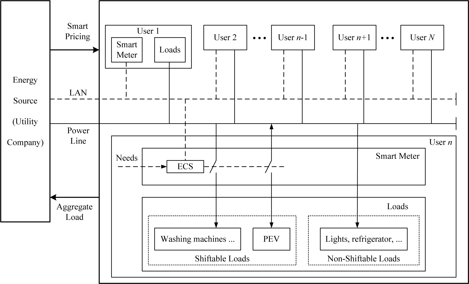
As in [5,9,13], we consider a smart power system with multiple load customers and a single energy source or utility company as part of the wholesale electricity market as shown in Figure 1. For all customers, we assume that they own smart meters with the ECS function to schedule household electricity consumption. All smart meters are connected to the power line coming from the utility company. All smart meters and the utility company can communicate with each other through a communication infrastructure such as a local area network (LAN). According to the above assumptions, power consumption model, energy cost model, and household load control will be formulated in this section.

2.1. Power Consumption Model

Consider a smart power supply system with a set of $\mathcal{N}=\{1,\dots ,N\}$ users that share an energy source. For each user n, let $l_n^h$ denote the total energy consumption of household appliances and loads at hour $h\in \mathscr{H}=\{1,\dots ,H\}$. For a daily operation of the grid, each time slot may take one hour and we have H = 24. The total daily load schedule for user n is denoted by $1_n\stackrel{\mathrm{\Delta }}{=}\left[l_n^1,\dots ,l_n^H\right]$, and the total load for all users during a time h can be described as:

$$L_h\stackrel{\mathrm{\Delta }}{=}{\displaystyle \sum _{n\in \mathcal{N}}{l}_n^h}$$

(1)

The daily peak and average load levels are calculated as:

$$L_{\mathrm{peak}}=\underset{h\in \mathscr{H}}{\max }{L}_h$$

(2)

and:

$$L_{\mathrm{avg}}=\frac{1}{H}{\displaystyle \sum _{h\in \mathscr{H}}{L}_h}$$

(3)

respectively. Therefore, the PAR in the load demand is:

$$\mathrm{PAR}=\frac{L_{\mathrm{peak}}}{L_{\mathrm{avg}}}=H\frac{{\max }_{h\in \mathscr{H}}{L}_h}{{\displaystyle {\sum }_{h\in \mathscr{H}}{L}_h}}$$

(4)

2.2. Energy Cost Model

The utility company obtains energy from multiple sources and sells it to the users. Energy cost model is cost function to determine the price at which the utility company sells energy to the customers. A smart cost function is important to provide incentive for users to follow a specific consumption behavior and minimize the impact of selfish behavior. Let C_h(L_h) be a cost function indicating the cost of generating or distributing electricity by the energy source as well as consuming electricity by users at each hour $h\in \mathscr{H}$. We make the following assumptions [13]:

• The cost functions are always increasing with respect to the total demand.

• The cost functions are strictly convex.

• When residential users buy energy from the utility company, we have C_h(L_h) > 0 for L_h > 0; when residential users sell energy back with their PEVs, we have C_h(L_h) < 0 for L_h < 0.

• At any given time h, the utility company will always make a profit, i.e., the price at which it buys energy from the residential users is always less than the price at which it sells.

Only increasing and strictly convex for cost functions are required for energy consumption scheduling without selling energy back in most literatures [5,8,9], and quadratic cost function:

$$C_h(L_h)=a_h{L}_h^2+b_h{L}_h+c_h$$

(5)

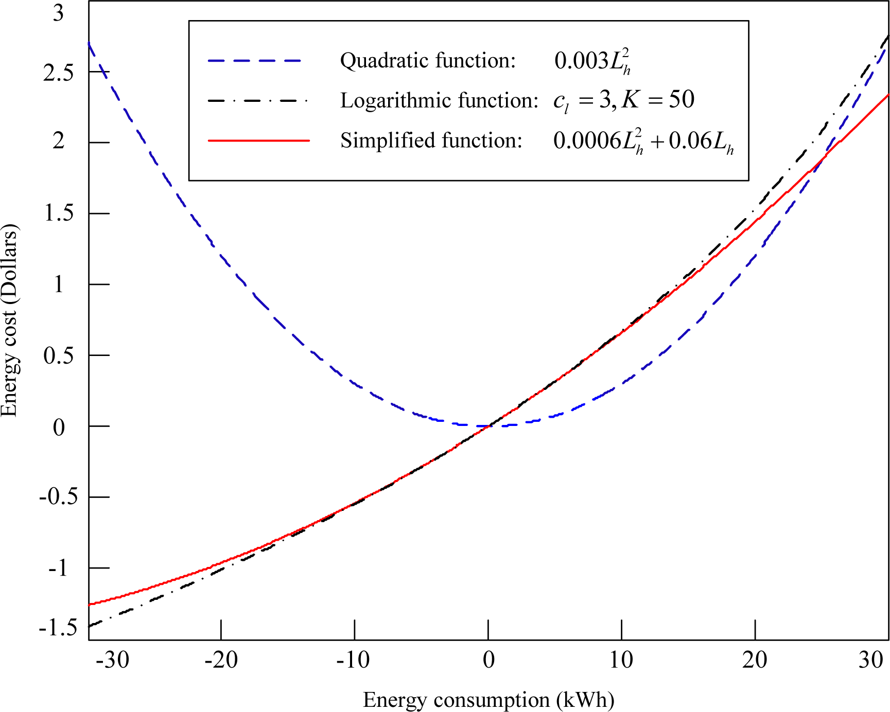
where a_h > 0, b_h ≥ 0, and c_h ≥ 0 are fixed parameters, for thermal generators is usually considered as the cost function. However, when the users can sell their energy back, they should be paid for their energy, that is C_h(L_h) < 0 for L_h < 0. A simple quadratic cost function, such as $C_h(L_h)=a_h{L}_h^2$, clearly does not satisfy this condition. Logarithmic cost functions were proposed to meet all of the four requirements in [13,30]. According to the logarithmic cost function:

$$C_h(L_h)=-c_l\log \left(1-\frac{L_h}{K}\right)$$

(6)

used in [13], where c_l > 0 is a cost coefficient and K is a parameter introduced to give cost values very close to the values given by a quadratic one, we employ a simplified cost function as:

$$C_h(L_h)={\widehat{a}}_h{L}_h^2+{\widehat{b}}_h{L}_h$$

(7)

where ${\widehat{a}}_h>0$ and ${\widehat{b}}_h>0$ are fix parameters. One can see that the simplified cost function in Equation (7) is included in the general quadratic cost function in Equation (5) and also can be Taylor expanded for the logarithmic cost Equation (6). However, since people normally used $C_h(L_h)=a_h{L}_h^2$ for their cost function [9] and logarithmic function is complicated, it is valuable to present the cost function in Equation (7) in this paper. The relationship among the cost functions in Equations (5)–(7) can be illustrated in Figure 2. It can be seen that the quadratic cost function can not describe the selling energy back case but the other two cost functions can. Moreover, the presented simplified cost function can approach the logarithmic cost function well to meet all the listed four assumptions well.

2.3. Household Load Control

Under the autonomous demand response paradigm [9], ECS in user’s smart meter seeks to schedule energy consumption such that the billing is minimized. For each user n, let ${\mathcal{A}}_n$ denote the set of household appliances such as lights, air conditioning, PEV, etc. For each appliance $a\in {\mathcal{A}}_n$, we define a load scheduling vector as:

$${\mathrm{x}}_{n,a}=\left[x_{n,a}^1,\dots ,x_{n,a}^h,\dots ,x_{n,a}^H\right]$$

(8)

where $x_{n,a}^h$ denotes the one-hour energy consumption that is scheduled for appliance a at hour h. It should be noted that $x_{n,a}^h$ is always a non-negative scalar for buying energy from the utility company as in [9] while it is a negative scalar for selling energy back to the utility company with PEV in this paper. Therefore, the total load of user n at hour h is calculated as:

$$l_n^h={\displaystyle \sum _{a\in A_n}{x}_{n,a}^h},h\in H$$

(9)

According to the illustration of household appliances as in Figure 1, each user has a set of non-shiftable and shiftable appliances. In our design, it is similar as in [9] that the designed energy consumption scheduler does not aim to change the amount of energy consumption, but instead to systematically manage the energy consumption of the shiftable appliances. Let E_a,n denote the total energy predetermined by appliance a belonging to user n. In addition, the user n selects the beginning time ${\alpha }_{n,a}\in \mathscr{H}$ and ending time ${\mathrm{\beta }}_{n,a}\in \mathscr{H}$, where ${\alpha }_{n,a}<{\mathrm{\beta }}_{n,a}$, that appliance a can be managed. Therefore, the following constraint mush hold:

$${\displaystyle \sum _{h={\alpha }_{n,a}}^{{\beta }_{n,a}}{x}_{n,a}^h}=E_{n,a}$$

(10)

and:

$$x_{n,a}^h=0,\forall h\in \mathscr{H}\backslash {\mathscr{H}}_{n,a}$$

(11)

where ${\mathscr{H}}_{n,a}\stackrel{\mathrm{\Delta }}{=}\{{\alpha }_{n,a},\dots ,{\mathrm{\beta }}_{n,a}\}$ denotes the available time slots for appliance a of the user n. The scheduling interval ${\mathscr{H}}_{n,a}$ should be equal to or longer than the normal time required for completing the operation for appliance a. For a shiftable appliance, the scheduling interval should be more than the normal requirement time. While, for a non-shiftable appliance, its scheduling interval is either a whole day with constant energy consumption (e.g., refrigerator) or equal to the normal requirement time in order to avoid further change to the plan.

It also can be concluded that daily energy consumption of all loads/appliances equals the total energy consumed by all appliances over 24 h, which leads to the following energy balance constraint:

$${\displaystyle \sum _{h\in \mathscr{H}}{L}_h}={\displaystyle \sum _{n\in \mathcal{N}}{\displaystyle \sum _{a\in {\mathcal{A}}_n}{E}_{n,a}}}$$

(12)

At the same time, the power level of each appliance a of the user n needs to be constrained. Let ${\gamma }_{n,a}^{\max }$ denote the maximum power level and ${\gamma }_{n,a}^{\min }$ denote the minimum power level. Then, it is clear that:

$${\gamma }_{n,a}^{\min }\le x_{n,a}^h\le {\gamma }_{n,a}^{\max },\forall h\in {\mathscr{H}}_{n,a}$$

(13)

Finally, by introducing vector x_n as energy consumption scheduling vector x_n,a for all appliances $a\in {\mathcal{A}}_n$, a feasible energy consumption scheduling set ${\mathcal{X}}_n$ corresponding to user n can be summarized as:

$${\mathcal{X}}_n=\left\{{\mathrm{x}}_n|{\displaystyle \sum _{h={\alpha }_{n,a}}^{{\mathrm{\beta }}_{n,a}}{x}_{n,a}^h=E_{n,a},x_{n,a}^h=0\forall h\in \mathscr{H}\backslash {\mathscr{H}}_{n,a},{\gamma }_{n,a}^{\min }\le x_{n,a}^h\le {\gamma }_{n,a}^{\max }\forall h\in {\mathscr{H}}_{n,a}}\right\}$$

(14)

3. Game-Theoretic Energy Consumption Scheduling

To achieve a lower energy cost, we suppose that residential users wish to preserve their privacy and are willing to share some information. According to the incentive electricity pricing set by the utility company, each user will try to adjust its electricity energy scheduling with the information that exchanges among the smart meters and the energy source. Game theory is able to capture the competitive behavior of the users. In this section, to minimize the energy cost, we will employ game theory to adjust electricity arrangements according to the demands of all residential users who are equipped with smart meters with ECS functionality.

3.1. Energy Cost Minimization

In terms of residential users, the purpose of getting involved in energy consumption scheduling is to reduce their electricity energy costs. Therefore, our goal is to find an efficient energy consumption scheduling in terms of minimizing the energy costs to all residential users, which can be expressed as the following optimization problem:

$$\underset{{\mathrm{x}}_n\in {\mathcal{X}}_n,\forall n\in \mathcal{N}}{\mathrm{minimize}}{\displaystyle \sum _{h=1}^H{C}_h}\left({\displaystyle \sum _{n\in \mathcal{N}}{\displaystyle \sum _{a\in {\mathcal{A}}_n}{x}_{n,a}^h}}\right)$$

(15)

Because the cost function C_h(·) is assumed to be strictly convex, problem in Equation (15) is a convex optimization and can be solved easily using convex programming techniques, such as interior point method (IPM) [9].

The optimization problems defined in Equation (15) can be solved to obtain an optimal solution for the given users and their energy schedules. However, once some users are selfish and interested only in optimizing their own costs, they might deviate from the centralized solution if they find new schedules with less costs. Moreover, it is important to find an approach that can be implemented with smart meters autonomously. Consequently, we need to calculate the billing tariffs for residential users.

3.2. Residential Billing Tariffs

Let b_n denote the daily billing amount that the utility company charges user $n\in \mathcal{N}$ at the end of each day. Then the billing tariff for all the users can be calculated as:

$${\displaystyle \sum _{n\in \mathcal{N}}{b}_n}={\displaystyle \sum _{h-1}^H{C}_h}\left({\displaystyle \sum _{n\in \mathcal{N}}{x}_{n,a}^h}\right)$$

(16)

In addition, we assume that users are charged proportional to their total daily energy consumption [9], which is consistent with the existing residential metering models. For arbitrary two user n and m, this proportional relationship can be presented as:

$$\frac{b_n}{b_m}=\frac{{\displaystyle \sum {}_{h=1}^H{l}_n^h}}{{\displaystyle \sum {}_{h=1}^H{l}_m^h}},\forall n,m\in \mathcal{N}$$

(17)

This feasible assumption can help analyzing tractable by directly relating each residential electricity billing to the total billing in Equation (16) in the smart power supply system.

Equation (17) can be rewritten as:

$$b_m=b_n\frac{{\displaystyle \sum {}_{h=1}^H{l}_m^h}}{{\displaystyle \sum {}_{h=1}^H{l}_n^h}}$$

(18)

Summing up both sides of the above equation for all users $m\in \mathcal{N}$, billing tariff for each user $n\in \mathcal{N}$ can be calculated as:

$$b_n=\frac{{\displaystyle \sum {}_{h=1}^H{l}_n^h}}{{\displaystyle {\sum }_{m\in \mathcal{N}}{\displaystyle \sum {}_{h=1}^H{l}_m^h}}}\left({\displaystyle \sum _{m\in \mathcal{N}}{b}_m}\right)={\Omega }_n{\displaystyle \sum _{h=1}^H{C}_h}\left({\displaystyle \sum _{m\in \mathcal{N}}{\displaystyle \sum _{a\in {\mathcal{A}}_m}{x}_{m,a}^h}}\right)$$

(19)

where:

$${\Omega }_n=\frac{{\displaystyle {\sum }_{a\in {\mathcal{A}}_m}{E}_{n,a}}}{{\displaystyle {\sum }_{m\in \mathcal{N}}{\displaystyle {\sum }_{a\in {\mathcal{A}}_m}{E}_{m,a}}}}$$

(20)

represents the proportion of energy consumed by user n, relative to the total energy consumed by all participated users. In other words, the electricity payment of each user not only depends on its own electricity consumption but also is related to others users’ electricity consumption.

According to the billing tariff in Equation (19), we have not considered any depreciation costs of household appliances. Although most household appliances could be neglected, such as the refrigerator and washer, the depreciation cost of the PEV’s battery can not be ignored in practice, especially when the battery is charged and discharged frequently [35,36] for storing and selling back the energy to the utility company. Because the normal charging and discharging for driving of the PEV have a smaller impact on its battery, we mainly consider the depreciation cost because of charing and discharging PEV’s battery frequently, i.e., depreciation cost of PEV’s battery for selling energy back to the utility company. For user $m\in \mathcal{N}$, let η_m(·) denote the depreciation cost of selling energy back. To keep the optimization problem in Equation (15) convex, the depreciation cost function is simply defined as a quadratic function:

$${\mathrm{\eta }}_m(l_{\mathrm{v}2\mathrm{g}})=a_{\mathrm{\eta }}{l}_{\mathrm{v}2\mathrm{g}}^2$$

(21)

where a_η is a positive parameter and l_v2g is the vehicle to grid (v2g) energy that is sold back to the utility company with PEVs. Then, the billing tariff in Equation (19) is revised to:

$$b_n={\Omega }_n{\displaystyle \sum _{h=1}^H{C}_h}\left({\displaystyle \sum _{m\in \mathcal{N}}{\displaystyle \sum _{a\in {\mathcal{A}}_m}{x}_{m,a}^h}}\right)+{\Phi }_n{\displaystyle \sum _{h=1}^H{\eta }_m}\left({\displaystyle \sum _{m\in \mathcal{N}}{x}_{m,\mathrm{v}2\mathrm{g}}^h}\right)$$

(22)

where $x_{m,\mathrm{v}2\mathrm{g}}^h$ represents the energy amount that is sold back by user m at time slot h. Because of $x_{m,\mathrm{v}2\mathrm{g}}^h$ is stored (positive charging load) and sold back (negative discharging load), one can see that it has no impact on the total consumed energy $E_m={\displaystyle {\sum }_{a\in {\mathcal{A}}_m}{E}_{m,a}}$of the user m. And Φ_n, similar to the proportion coefficient of Ω_n, is defined as:

$${\Phi }_n=\frac{E_{n,\mathrm{v}2\mathrm{g}}}{{\displaystyle {\sum }_{m\in \mathcal{N}}{E}_{m,\mathrm{v}2\mathrm{g}}}},E_{n,\mathrm{v}2\mathrm{g}}={\displaystyle \sum _{h={\alpha }_{n,\mathrm{v}2\mathrm{g}}}^{{\mathrm{\beta }}_{n,v2g}}{x}_{n,\mathrm{v}2\mathrm{g}}^h,E_{m,\mathrm{v}2\mathrm{g}}=}{\displaystyle \sum _{h={\alpha }_{m,\mathrm{v}2\mathrm{g}}}^{{\mathrm{\beta }}_{m,v2g}}{x}_{m,\mathrm{v}2\mathrm{g}}^h}$$

(23)

which represents the proportion of energy sold back by user n, relative to the total energy sold back by all users.

3.3. Energy Consumption Game

Naturally, the energy consumption game among users can be defined as:

• Players: Users in the set $\mathcal{N}$.

• Strategies: Each user $n\in \mathcal{N}$ selects its energy consumption strategy by scheduling appliance $a\in {\mathcal{A}}_n$ to maximize its payoff.

• Payoffs: P_n(x_n; x_−n) for each user $n\in \mathcal{N}$ is defined as:

  $$P_n({\mathrm{x}}_n;{\mathrm{x}}_{-n})=-b_n=-{\Omega }_n{\displaystyle \sum _{h=1}^H{C}_h}\left({\displaystyle \sum _{m\in \mathcal{N}}{\displaystyle \sum _{a\in {\mathcal{A}}_m}{x}_{m,a}^h}}\right)-{\Phi }_n{\displaystyle \sum _{h=1}^H{\mathrm{\eta }}_m}\left({\displaystyle \sum _{m\in \mathcal{N}}{x}_{m,\mathrm{v}2\mathrm{g}}^h}\right)$$

  where ${\mathrm{x}}_{-n}\stackrel{\mathrm{\Delta }}{=}[{\mathrm{x}}_1,\cdots ,{\mathrm{x}}_{n-1},{\mathrm{x}}_{n+1},\cdots ,{\mathrm{x}}_N]$ denotes the energy consumption schedules for all users except the user n.

Based on the definitions of the strategies and payoffs in the above game, all users will try to schedule their household appliances to minimize their electricity payments until a Nash equilibrium of the game is reached:

• Nash equilibrium: Consider the game played among a set $\mathcal{N}$ of players. The energy consumption scheduling ${\mathrm{x}}_n\in {\mathcal{X}}_n$ for each user $n\in \mathcal{N}$ form a unique Nash equilibrium if and only if we have:

  $$P_n({\mathrm{x}}_n^{*};{\mathrm{x}}_{-n}^{*})\ge P_n({\mathrm{x}}_n;{\mathrm{x}}_{-n}^{*})$$

  (24)

Once the energy consumption game is at its unique Nash equilibrium, no one will benefit by deviating from ${\mathrm{x}}_n^{*},\forall n\in \mathcal{N}$. The proof of existence and uniqueness of Nash equilibrium in Equation (24) can be found in [13]. And the proof of unique Nash equilibrium of the game is also the optimal solution of the energy cost minimization problem can be processed similarly as in [9].

4. Simulation Results

In this section, simulation results will be presented to show the feasibility and effectiveness of the proposed residential energy consumption game. In addition, the programmed algorithm in Matlab to solve the Nash equilibrium in Equation (24) is referred to as Algorithm 1 in [9], which is mainly based on iteration by using IPM. Further, the conditions under which people would like to sell energy back to the utility company through their PEVs will also be discussed.

4.1. Residential Users Having Household Appliances and Plug-in Electric Vehicles

In the simulation, we consider a small SG system consisting of a utility company and five users that subscribe to the ECS services. For simplicity, we assume that each user could have two non-shiftable household appliances, i.e., refrigerator and lights, and three shiftable household appliances, i.e., dishwasher, washing machine and PEV. Daily electricity energy consumption of each residential load is assumed as in

Table 1. Daily electricity consumption of each residential load (kW·h).

Users	Refrigerator	Lights	Washing machine	PEV	Dishwasher
1	1.32	1.3	1.49	14.4	0
2	1.32	1.0	1.30	14.4	1.44
3	1.32	0.8	1.49	14.4	1.44
4	1.32	1.0	1.49	14.4	1.44
5	1.32	1.2	1.49	0	1.44

and working time setting of household appliances except PEV is assumed as in

Table 2. Working time of household appliances except plug-in electric vehicle: for the case without energy consumption scheduling function deployment, each appliance is assumed to start operation right at the initial time; for the case with energy consumption scheduling function deployment, the timing for the operation of each shiftable appliance is determined by the game result.

Appliances	Refrigerator	Lights	Washing machine	Dish-washer
Time interval	1:00–24:00	18:00–24:00	18:00–23:00	8:00–10:00, 20:00–22:00
Initial time	1:00	18:00	21:00	8:00 and 20:00
Time duration (h)	24	6	1	1 at each interval

. For non-shiftable loads, we assume that each refrigerator is used throughout the day and lights are on from 6:00 PM to 12:00 PM. For a shiftable load washing machine, we assume it will work for 1 h at any time between 6:00 PM and 11:00 PM. For a shiftable load dishwasher, it will work 2 h, 1 h between 8:00 AM and 10:00 AM and 1 h between 8:00 PM and 10:00 PM, respectively. For a shiftable load PEV, we assume all PEVs owned by the residential users are equipped with identical batteries, and the simulation parameters based on real-world data of existing PEVs [37–40] for the batteries are listed as in

Table 3. Parameters for battery of household plug-in electric vehicle: battery is assumed to be charged right at the initial time for the case without energy consumption scheduling function deployment; for the case with energy consumption scheduling function deployment, the timing for charging of each plug-in electric vehicle is determined by the game result; the discharging power level, discharging time interval, and depreciation coefficient is only valid with energy consumption scheduling and discharging case.

Items	Values	Items	Values
Battery capacity	20 kW•h	Charging/Discharging efficient	92%
Charging power	6 kW	Depreciation coefficient aη	0.00032
Discharging power	7 kW	Working time interval	1:00–7:00, 20:00–24:00
Discharging depth	80%	Initial working time	20:00

. The capacity of each battery is 20 kW·h. We assume that PEV’s battery will be charged to maximum capacity at 7:00 AM for driving in daytime, the energy consumption for driving is 14.4 kW·h as shown in Table 1. The battery will not be connected to the grid when the user is not at home, i.e., from 7:00 AM to 20:00 PM. Once the user is back home, the PEV can be charged and discharged from 8:00 PM to 1:00 AM the day after and only can be charged from 1:00 AM to 7:00 AM the day after. The maximum charging and discharging power level of the battery is 6 kW and 7 kW, respectively; coefficient of charging and discharging is assumed to be 92%. The maximum discharging depth of the battery is 80%, which means at least 4 kW·h has to be kept in the battery during discharging. In addition, according to Equation (21), the depreciation cost function of discharging PEV is selected as:

$${\mathrm{\eta }}_{\mathrm{PEV}}(l_{\mathrm{v}2\mathrm{g}})=0.00032l_{\mathrm{v}2\mathrm{g}}^2$$

(25)

The energy cost function is selected as depicted in Equation (7). Referring the cost functions selected in [9] that $C_{h,\mathrm{day}}=0.003L_h^2$ (Dollars) during daytime hours, i.e., from 8:00 AM to 12:00 PM, and $C_{h,\mathrm{night}}=0.002L_h^2$ (Dollars) during the night, i.e., from 12:00 PM to 8:00 AM the day after; the cost functions in this paper are defined as:

$$C_{h,\mathrm{day}}(L_h)=0.00084L_h^2+0.064L_h$$

(26)

$$C_{h,\mathrm{night}}(L_h)=0.0004L_h^2+0.045L_h$$

(27)

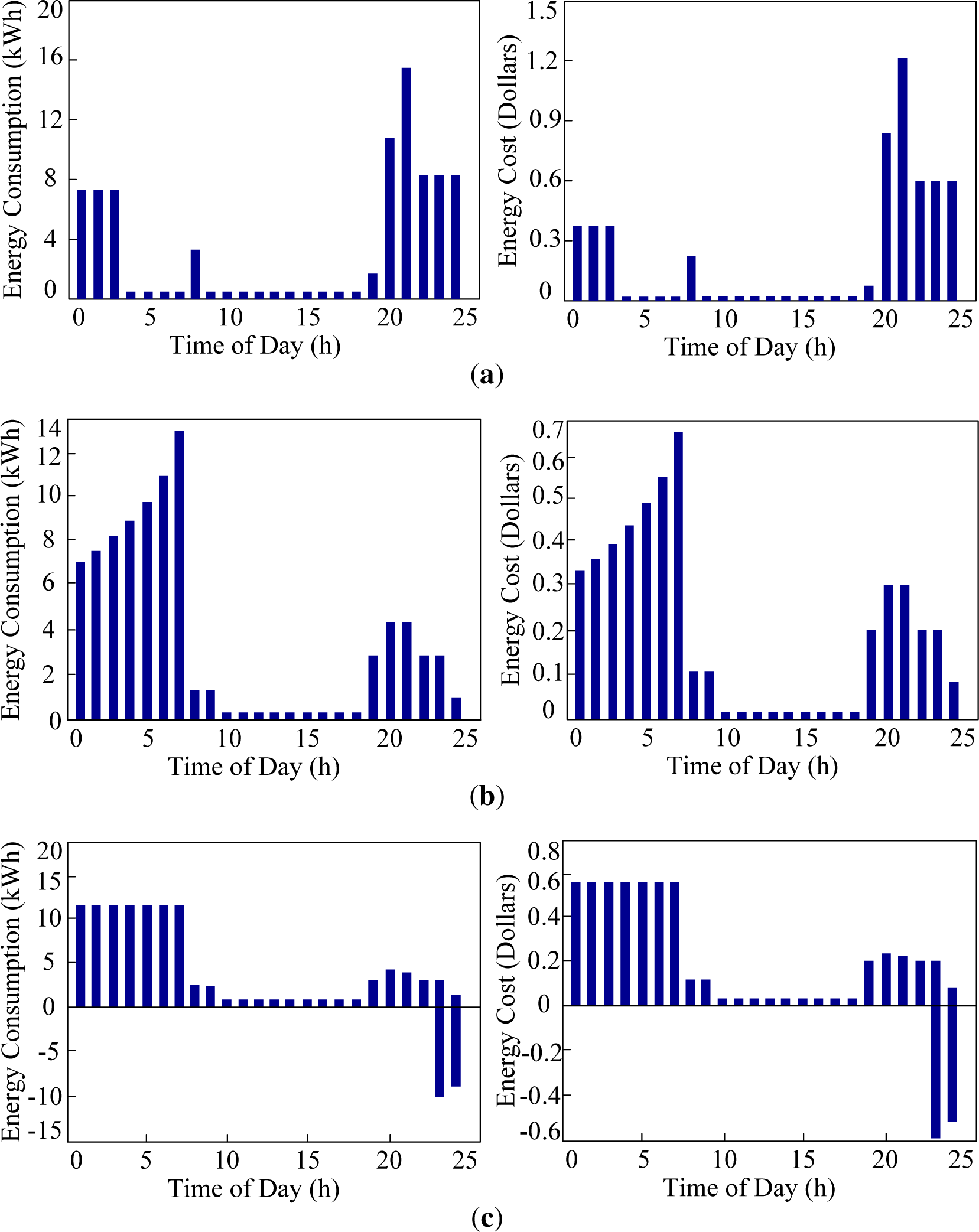
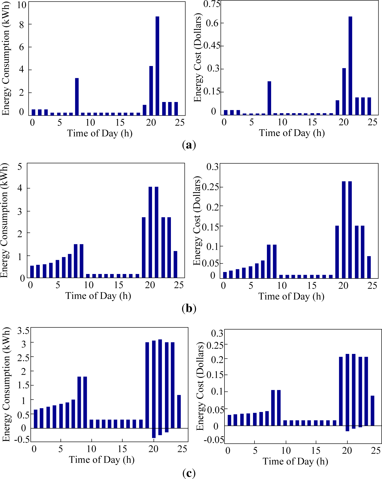
The simulation results on scheduled energy consumption and corresponding cost of the aggregate five users having household appliances and PEVs are shown in Figure 3, for the cases without ECS deployment, with ECS deployment but without discharging battery to sell energy back, and with ECS deployment and discharging battery to sell energy back. One can see that when ECS functions are not deployed, the aggregate cost is 5.29 Dollars and the PAR is 4.36. Once the ECS based on game theory is implemented, the aggregate cost reduces to 4.76 Dollars and PAR is reduced to 3.35. Moreover, when the residential users sell energy back to the utility company by storing and discharging electricity energy with their PEVs, the aggregate cost reduces to 3.28 Dollars and the PAR reduces to 2.63 further. The decreasing of PAR will benefit the utility company, therefore the utility company should encourage users to participate in the game.

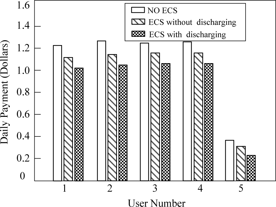
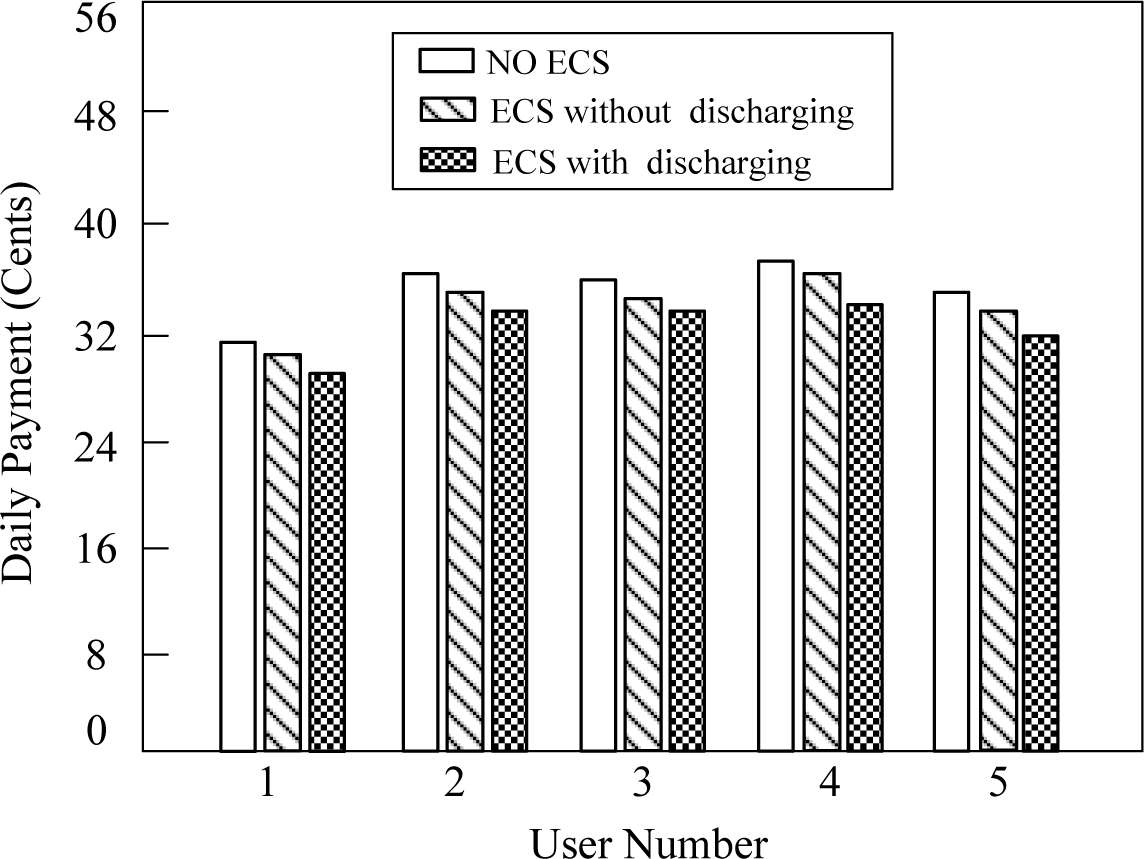
While the proposed ECS based on game theory leads to less total cost and lower PAR in the aggregate load from the five users, it is also beneficial for each residential user. The daily payments for each user in different cases are shown in Figure 4. One can see that the payments of each user decrease monotonically from the case without ECS, to the case with ECS but without selling energy back, and to the case with ECS and selling energy back. Even for User 5, who dose not own a PEV, his/her energy payments decrease monastically because of participating in the game. Therefore, all the users will benefit and be willing to take part in the game.

4.2. Chinese Residential Users Having Household Appliances and Plug-in Bicycles

For Chinese residential users who already own household appliances and PEBs other than PEVs, the settings for household appliances are identical with the previous simulation. For shiftable load PEBs, we also assume all PEBs are equipped with identical batteries, and their simulation parameters [41,42] are listed as in

Table 4. Parameters for battery of household plug-in electric bicycle: battery is assumed to be charged right at the initial time for the case without energy consumption scheduling function deployment; for the case with energy consumption scheduling function deployment, the timing for the operation of each shiftable appliance is determined by game result; the discharging power level, discharging time interval, and depreciation coefficient is only valid with energy consumption scheduling and discharging case.

Items	Values	Items	Values
Battery Capacity	0.96 kW•h	Charging/Discharging Efficient	92%
Charging power	0.4 kW	Depreciation coefficient aη	0.0008
Discharging power	0.24 kW	Working time interval	1:00–7:00, 20:00–24:00
Discharging depth	60%	Initial working time	20:00

. The capacity of each battery is reduced to 0.94 kW·h which will be fully charged at 7:00 AM. The energy consumed for driving is 0.7 kW·h. The time settings for charging and discharging are also the same with the case of PEVs. The maximum charging and discharging power level of the battery is 0.4 kW and 0.24 kW, respectively; the coefficient of charging and discharging is also set to 92%. The maximum discharging depth of the battery is 60%. In addition, the depreciation coefficient of discharging PEBs is selected as 0.0008.

The corresponding simulation results are shown in Figures 5 and 6, for the cases without ECS deployment, with ECS deployment but without discharging battery to sell energy back, and with ECS deployment and discharging battery to sell energy back. One can see that when ECS functions are not deployed, the aggregate cost is 1.74 Dollars and the PAR is 7.77. Once the ECS based on game theory is implemented, the aggregate cost reduces to 1.68 Dollars and PAR is reduces to 3.57. Moreover, when the residential users sell energy back to the utility company by storing and discharging electricity energy with their PEBs, the aggregate cost reduces to 1.61 Dollars and the PAR reduces to 2.84 further. In addition, the daily payments for each user will decrease monotonically from the case without ECS, to the case with ECS but without selling energy back, and to the case with ECS and selling energy back. It is apparent that the decreasing amplitude becomes smaller comparing to residential users having PEVs. The reasons are a significantly smaller battery capacity, smaller discharging depth and larger depreciation cost of battery because of discharging energy to the utility company. However, as long as benefits exist, people would like to take part in the game and selling energy back to the utility company.

4.3. Discussion on Discharging Predication of the Plug-In Electric Vehicle’s Battery

According to the previous two sets of simulation results, we have known that both the utility company and residential users will benefit by deploying the proposed ECS based on game theory. Although the two simulation cases show that people would like to sell energy back to the utility company, one should notice that residential users owning PEBs benefit only a little more when comparing the case with ECS and discharging to the case with ECS but without discharging. In practice, one additional investment, such as an inverter, needed for selling energy back, or there would no longer be a profit. Therefore, people will not be willing to sell energy back by discharging their batteries. To describe this issue clearly, for a random user, we can calculate the profit of selling energy back by discharging a battery as:

$${\mathrm{\Delta }}_{\mathrm{P}}=C_{\mathrm{discharge}}(l_{\mathrm{v}2\mathrm{g}})-C_{\mathrm{charge}}(l_{\mathrm{v}2\mathrm{g}})-\mathrm{\eta }(l_{\mathrm{v}2\mathrm{g}})$$

(28)

where C_discharge (l_v2g), C_charge (l_v2g) and η(l_v2g) denote the payment from the utility company for selling energy back, the cost to charge the energy amount and the overall depreciation cost of storing and selling energy back, respectively. Therefore, generally speaking, only when the profit ∆_p is a large enough positive incentive number, would the user like to sell energy back using his/her PEV. According to [43], the cost of battery degradation can be approximately 26.25 Cents per kW·h of throughput in the 1500 cycle lifetime scenario and substantially lower at 6.45 Cents per kW·h of throughput in the 5300 cycle scenario. In other words, if discharging price minus charging price is less than 6.45 Cents per kW·h in the 5300 cycle scenario, people would not do sell energy back by using his/her PEV’s battery. From the perspective of utility companies, once they find that the residential users selling energy back can help decreasing PAR, they would like to encourage residential users to do it. If necessary, the utility company would be willing to present a special energy price for the residential users who could store and sell electricity energy back by using their PEVs at proper timings, such as electricity price subsidies which have been already implemented for distributed wind farms [44] or photovoltaic plants [45].

5. Conclusions

In this paper, we have presented a game-theoretic approach to schedule the energy consumption of residential users automatically in the presence of bidirectional energy trading by allowing the residents to buy and sell energy from/to the utility company with their PEVs. Simulation results show that the proposed DSM strategy can reduce the aggregate cost of the five residential users from 4.76 Dollars to 3.28 Dollars and the PAR from 3.35 to 2.63, once users sell energy back to the utility company by using their PEVs, which can benefit both residential users and utility company further. In addition, the analysis on the discharging depreciation of PEV’s battery shows that the utility company would need to provide special electricity price subsides to encourage residential users to store and sell electricity energy back by using their PEVs at proper timings.

References

- Eberle, U.; Muller, B.; von Helmolt, R. Fuel cell electric vehicles and hydrogen infrastructure: Status 2012. Energy Environ. Sci 2012, 5, 8780–8792. [Google Scholar]
- Multin, M.; Allerding, F.; Schmeck, H. Integration of electric vehicles in smart homes—an ICT-based solution for V2G scenarios, Proceedings of the IEEE PES Innovative Smart Grid Technologies, Washington, DC, USA, 16–20, January 2012; pp. 1–8.
- Di Silvestre, M.L.; Riva Sanseverino, E.; Zizzo, G.; Graditi, G. An optimization approach for efficient management of EV parking lots with batteries recharging facilities. J. Ambient Intell. Hum. Comput 2013, 4, 641–649. [Google Scholar]
- Baharlouei, Z.; Hashemi, M.; Narimani, H.; Mohsenian-Rad, H. Achieving optimality and fairness in autonomous demand response: Benchmarks and billing mechanisms. IEEE Trans. Smart Grid 2013, 4, 968–975. [Google Scholar]
- Samadi, P.; Mohsenian-Rad, H.; Schober, R.; Wong, V.W.S. Advanced demand side management for the future smart grid using mechanism design. IEEE Trans. Smart Grid 2012, 3, 1170–1180. [Google Scholar]
- Palensky, P.; Dietrich, D. Demand side management: Demand Response, intelligent energy systems, and smart loads. IEEE Trans. Ind. Inform 2011, 7, 381–388. [Google Scholar]
- Siano, P.; Graditi, G.; Atrigna, M.; Piccolo, A. Designing and testing decision support and energy management systems for smart homes. J. Ambient Intell. Hum. Comput 2013, 4, 651–661. [Google Scholar]
- Baharlouei, Z.; Hashemi, M. Efficiency-fairness trade-off in privacy-preserving autonomous demand side management. IEEE Trans. Smart Grid 2014, 5, 799–808. [Google Scholar]
- Mohsenian-Rad, A.-H.; Wong, V.W.S.; Jatskevich, J.; Schober, R.; Leon-Garcia, A. Autonomous demand-side management based on game-theoretic energy consumption scheduling for the future smart grid. IEEE Trans. Smart Grid 2010, 1, 320–331. [Google Scholar]
- Zhang, X. Optimal scheduling of critical peak pricing considering wind commitment. IEEE Trans. Sustain. Energy 2014, 5, 637–645. [Google Scholar]
- Deng, R.; Yang, Z.; Chen, J.; Asr, N.R.; Chow, M.-Y. Residential energy consumption scheduling: A coupled-constraint game approach. IEEE Trans. Sustain. Energy 2014, 5, 1340–1350. [Google Scholar]
- Ma, K.; Hu, G.; Spanos, C.J. Energy consumption control via real-time pricing feedback in smart grid. IEEE Trans. Control Syst. Technol 2014, 22, 1907–1914. [Google Scholar]
- Soliman, H.M.; Leon-Garcia, A. Game-theoretic demand-side management with storage devices for the future smart grid. IEEE Trans. Smart Grid 2014, 5, 1475–1485. [Google Scholar]
- Bu, S.; Yu, F.R. A game-theoretical scheme in the smart grid with demand-side management: Towards a smart cyber-physical power infrastructure. IEEE Trans. Emerg. Top. Comput 2013, 1, 22–32. [Google Scholar]
- Kim, B.-G.; Ren, S.; Schaar, M.; Lee, J.-W. Bidirectional energy trading and residential load scheduling with electric vehicles in the smart grid. IEEE J. Sel. Areas Commun 2013, 31, 1219–1234. [Google Scholar]
- Nguyen, P.H.; Kling, W.L.; Ribeiro, P.F. A game theory strategy to integrate distributed agent-based functions in smart grids. IEEE Trans. Smart Grid 2013, 4, 568–576. [Google Scholar]
- Saad, W.; Han, Z.; Poor, H.V.; Basar, T. Game theoretic methods for the smart grid: An overview of microgrid systems, demand-side management, and smart grid communications. IEEE Signal Process. Mag 2012, 9, 86–105. [Google Scholar]
- Tushar, M.H.K.; Assi, C.; Maier, M.; Uddin, M.F. Smart microgrids: Optimal joint scheduling for electric vehicles and home appliances. IEEE Trans. Smart Grid 2014, 5, 239–250. [Google Scholar]
- Yang, P.; Tang, G.; Nehorai, A. A game-theoretic approach for optimal time-of-use electricity pricing. IEEE Trans. Power Syst 2013, 28, 884–892. [Google Scholar]
- Tushar, W.; Saad, W.; Poor, H.V.; Smith, D.B. Economics of electric vehicle charging: A game theoretic approach. IEEE Trans. Smart Grid 2012, 3, 1767–1778. [Google Scholar]
- Tushar, W.; Zhang, J.A.; Smith, D.B.; Poor, H.V.; Thiebaux, S. Prioritizing consumers in smart grid: A game theoretic approach. IEEE Trans. Smart Grid 2014, 5, 1429–1438. [Google Scholar]
- Maharjan, S.; Zhu, Q.; Zhang, Y.; Gjessing, S.; Basar, T. Dependable demand response management in the smart grid: A Stackelberg game approach. IEEE Trans. Smart Grid 2013, 4, 120–132. [Google Scholar]
- Nguyen, H.K.; Song, J.B. Optimal charging and discharging for multiple PHEVs with demand side management in vehicle-to-building. J. Commun. Netw 2012, 14, 662–671. [Google Scholar]
- Wang, Y.; Saad, W.; Han, Z.; Poor, H.V.; Basar, T. A game-theoretic approach to energy trading in the smart grid. IEEE Trans. Smart Grid 2014, 5, 1439–1450. [Google Scholar]
- Atzeni, I.; Ordonez, L.G.; Scutari, G.; Palomar, D.P.; Fonollosa, J.R. Demand-side management via distributed energy generation and storage optimization. IEEE Trans. Smart Grid 2013, 4, 866–876. [Google Scholar]
- Atzeni, I.; Ordonez, L.G.; Scutari, G.; Palomar, D.P.; Fonollosa, J.R. Noncooperative and cooperative optimization of distributed energy generation and storage in the demand-side of the smart grid. IEEE Trans. Signal Process 2013, 61, 2454–2472. [Google Scholar]
- Atzeni, I.; Ordonez, L.G.; Scutari, G.; Palomar, D.P.; Fonollosa, J.R. Noncooperative day-ahead bidding strategies for demand-side expected cost minimization with real-time adjustments: A GNEP approach. IEEE Trans. Signal Process 2014, 62, 2397–2412. [Google Scholar]
- Chen, H.; Li, Y.; Louie, R.H.Y.; Vucetic, B. Autonomous demand side management based on energy consumption scheduling and instantaneous load billing: An aggregative game approach. IEEE Trans. Smart Grid 2014, 5, 1744–1754. [Google Scholar]
- Chai, B.; Chen, J.; Yang, Z.; Zhang, Y. Demand response management with multiple utility companies: A two-level game approach. IEEE Trans. Smart Grid 2014, 5, 722–731. [Google Scholar]
- Fadlullah, Z.M.; Quan, D.M.; Kato, N.; Stojmenovic, I. GTES: An optimized game-theoretic demand-side management scheme for smart grid. IEEE Syst. J 2014, 8, 588–597. [Google Scholar]
- Fairley, P. China’s cyclisists take charge: Electric bicycles are sellig by the millions despite efforts to ban them. IEEE Spectr 2005, 42, 54–59. [Google Scholar]
- Zhang, H.; Shaheen, S.A.; Chen, X. Bicycle evolution in China: From the 1900s to the present. Int. J. Sustain. Transp 2014, 8, 317–335. [Google Scholar]
- Erkin, Z.; Troncoso-Pastoriza, J.R.; Lagendijk, R.L.; Perez-Gonzalez, F. Privacy-preserving data aggregation in smart metering systems: An overview. IEEE Trans. Signal Process. Mag 2013, 30, 75–86. [Google Scholar]
- Sate Grid Corpration of China. On service work for grid-connected distributed generation. Solar Energy 2013, 6, 6–7, In Chinese.
- Peterson, S.B.; Apt, J.; Whitacre, J.F. Lithium-ion battery cell degradation resulting from realistic vehicle and vehicle-to-grid utilization. J. Power Sources 2010, 195, 2385–2392. [Google Scholar]
- Guenther, C.; Schott, B.; Hennings, W.; Waldowski, P.; Danzer, M.A. Model-based investigation of electric vehicle battery aging by means of vehicle-to-grid scenario simulations. J. Power Sources 2013, 239, 604–610. [Google Scholar]
- Sun, B.; Liao, Q.; Xie, P.; Zhou, G.; Shi, Q.; Ge, H. A cost-benefit analysis model of vehicle-to-grid for peak shaving. Power Syst. Technol 2012, 36, 30–34. [Google Scholar]
- Luo, Z.; Hu, Z.; Song, Y.; Xu, Z.; Yang, Y.; Liu, H. Coordinated charging and discharging of large-scale plug-in electric vehicles with cost and capacity benefit analysis. Autom. Electr. Power Syst 2012, 36, 19–26. [Google Scholar]
- Matthe, R.; Eberle, U. The voltec system-energy storage and electric propulsion. In Lithium-Ion Batteries: Advances and Applications; Pistoia, G., Ed.; Elsevier: Amsterdam, The Netherlands, 2014; pp. 151–176. [Google Scholar]
- Warner, J. Lithium-Ion Battery Packs for EVs. In Lithium-Ion Batteries: Advances and Applications; Pistoia, G., Ed.; Elsevier: Amsterdam, The Netherlands, 2014; pp. 127–150. [Google Scholar]
- Muetze, A.; Tan, Y.C. Electric bicycle—A performance evaluation. IEEE Ind. Appl. Mag 2007, 13, 12–21. [Google Scholar]
- Ke, W.; Zhang, N. Charging models and the performance of battery packs for electric bicycles, Proceedings of the Australasian Universities Power Engineering Conference, Perth, Australia, 9–12, December 2007; pp. 1–4.
- White, C.D.; Zhang, K.M. Using vehicle-to-grid technology for frequency regulation and peak-load reduction. J. Power Sources 2011, 196, 3972–3980. [Google Scholar]
- Abadie, L.M.; Chamorro, J.M. Valuation of wind energy projects: A real options approach. Energies 2014, 7, 3218–3255. [Google Scholar]
- Chen, Z.; Su, S.I. Photovoltaic supply chain coordination with strategic consumers in China. Renew. Energy 2014, 68, 236–244. [Google Scholar]