Dynamic Simulation of a CPV/T System Using the Finite Element Method

Abstract

The aim of this paper is the determination of a concentrating thermo-photovoltaic (CPV/T) system dynamic model by means of the finite element method (FEM). The system consist of triple-junction InGaP/InGaAs/Ge (indium-gallium phosphide/indium-gallium-arsenide/germanium) solar cells connected to a metal core printed circuit board (MCPCB) placed on a coil circuit used for the thermal energy recovery. In particular, the main aim is to determine the fluid outlet temperature. It is evaluated corresponding both to a constant cell temperature equal to 120 °C, generally representing the maximum operating temperature, and to cell temperature values instantly variable with the direct normal irradiation (DNI). Hence, an accurate DNI analysis is realized adopting the Gordon-Reddy statistical model. Using an accurate electric model, the cell temperature and efficiency are determined together with the CPV/T module electric and thermal powers. Generally, the CPV system size is realized according to the user electric load demand and, then, it is important to evaluate the necessary minimum concentration ratio (C_min), the limit of CPV system applicability, in order to determine the energy convenience profile. The fluid outlet temperature can be then obtained by the FEM analysis to verify if a CPV/T system can be used in solar heating and cooling applications.

1. Introduction

In concentrating photovoltaic systems (CPV), sunlight is concentrated on the solar cells by means of optical devices [1]. Higher temperatures are also reached [2] and this affects the electric performance, but also allows a high thermal energy recovery. The concentration systems that use triple-junction cells are less affected by the temperature increase, thus preserving a good electric efficiency [3]. Hence, the concentrating thermo-photovoltaic systems (CPV/T) allow one to not only obtain electric energy but also thermal energy. Systems which recover thermal energy from GaAs cell arrays are evaluated in [4]. In [5] the concentrating system thermal energy is used to supply a LiBr/H₂O single-effect absorption heat pump. In [6] a concentrating dish is designed and connected to a system of evacuated tubes to obtain a more efficient thermal energy production. In [7] the fluid which cools the cells is accumulated in a tank. A CPV/T system linked to an organic Rankine cycle in order to increase the electricity production is studied in [8], where the thermal energy obtained with a recovery system is supplied to a low-boiling fluid that allows an additional production of electric energy. A CPV/T system coupled with an air conditioning plant in order to separate latent load from sensitive load is shown in [9]. Referring to the electric, heating and cooling loads of a domestic user, in [10] the design and model of a concentrating photovoltaic thermal system are studied. Moreover, in [11] the optimized value of the concentration factor able to decrease the CPV/T system size and to provide a fluid outlet temperature, that satisfies the thermal and cooling demands, is determined in each working condition. Hence, there are different CPV/T systems that allow one to obtain a combined energy production, but there is not yet a standard configuration of these systems. In this paper the main aim is to determine by means of the finite element method (FEM) a dynamic model of a CPV/T system where the fluid cooling the cells flows in a coil circuit supplied by a pump. All this in order to determine the refrigerant fluid temperature corresponding to variable DNI values and then to verify the possibility to use a CPV/T system in solar heating and cooling applications.

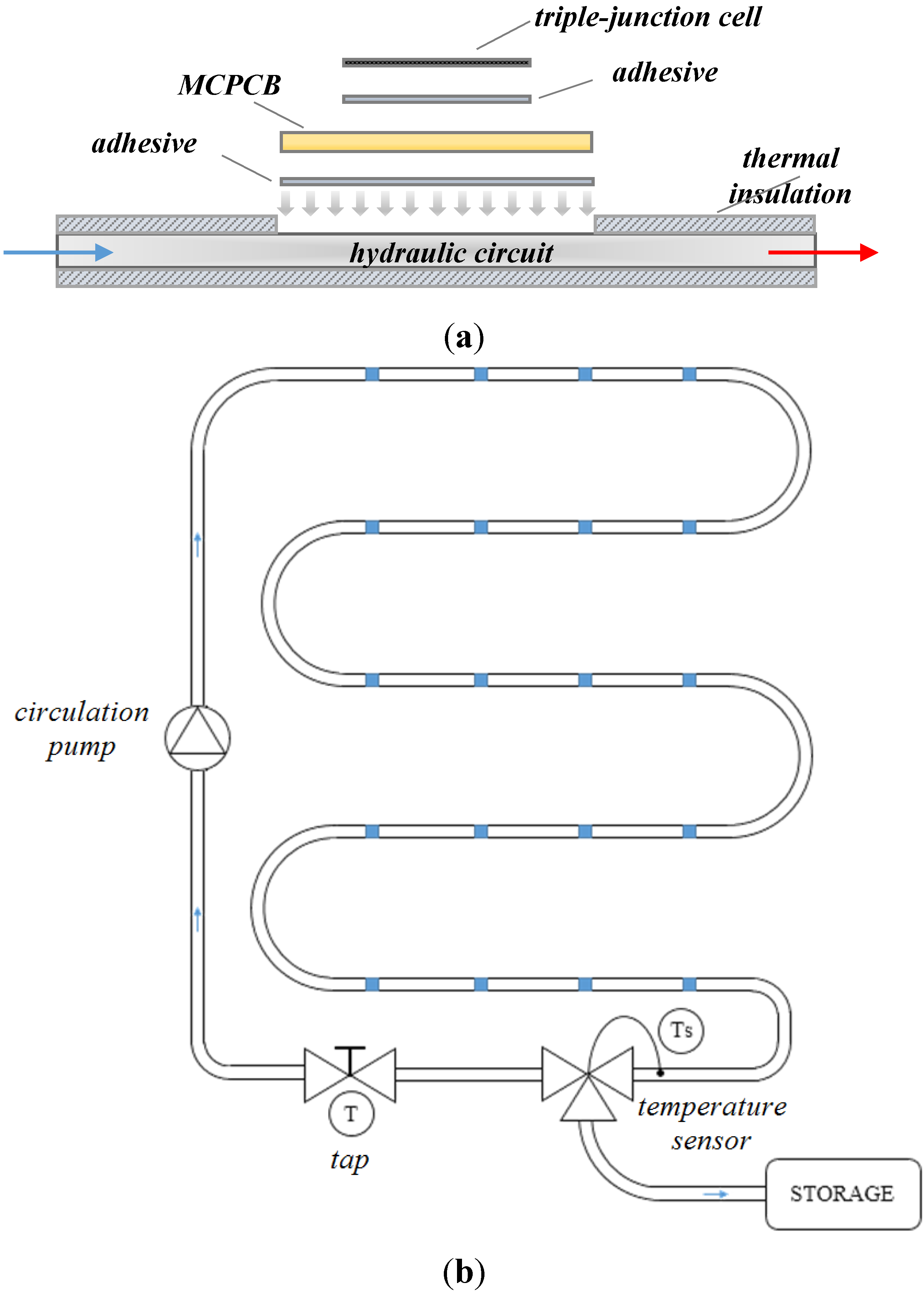
2. CPV/T System Description

The CPV systems allows an increase in the electric power and efficiency in comparison with a traditional silicon photovoltaic system by means of optical components (Fresnel lenses, parabolic mirrors, etc.) which concentrate the sunlight on high efficiency multi-junction solar cells. This technology allows the conversion of higher area of the electromagnetic solar spectrum thanks to the combination of different band-gap semiconductor layers. The system analyzed in this paper consist of triple-junction solar cells (InGaP/InGaAs/Ge). The cell is applied by means of an adhesive on a Metal Core Printed Circuit Board (MCPCB, Figure 1a), placed on a copper coil circuit properly sized for the thermal energy recovery (Figure 1b), where a fluid, usually water and glycol, flows. The size of the heat recovery system has been realized considering empirical criteria that include the analysis of friction losses, the minimum and maximum speed of refrigerant flow and the Reynolds number in order to prevent turbulent energy dissipations. According to these factors, a pipe diameter of 20 mm and a volumetric flow rate of 0.2 m³/h have been determined. In particular, a single CPV/T module of twenty multi-junction cells, able to supply to a domestic user an electric power of about 500 W if a high concentration ratio is considered, has been analyzed. Specific details about the optics and the solar tracking system have been considered in the parameters of the model.

Figure 1. (a) Schematic view of a CPV/T system; and of (b) a heat recovery coil circuit.

Figure 1. (a) Schematic view of a CPV/T system; and of (b) a heat recovery coil circuit.

3. CPV/T System Dynamic Model

The main aim is the determination of a model that links the input variables, such as solar radiation and solar cell parameters, with the output variables in order to quantify the cell efficiency and temperature and the electric and thermal powers under concentrated light. This analysis allows determination of the CPV/T system performance also in terms of refrigerant fluid temperature.

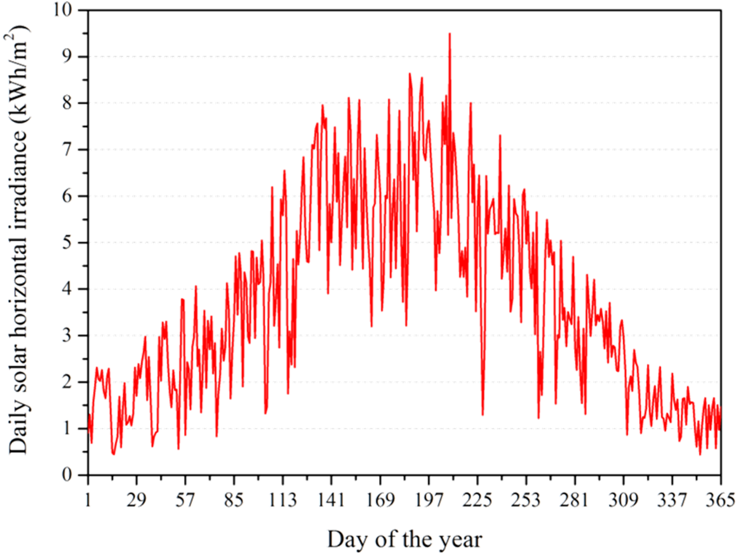
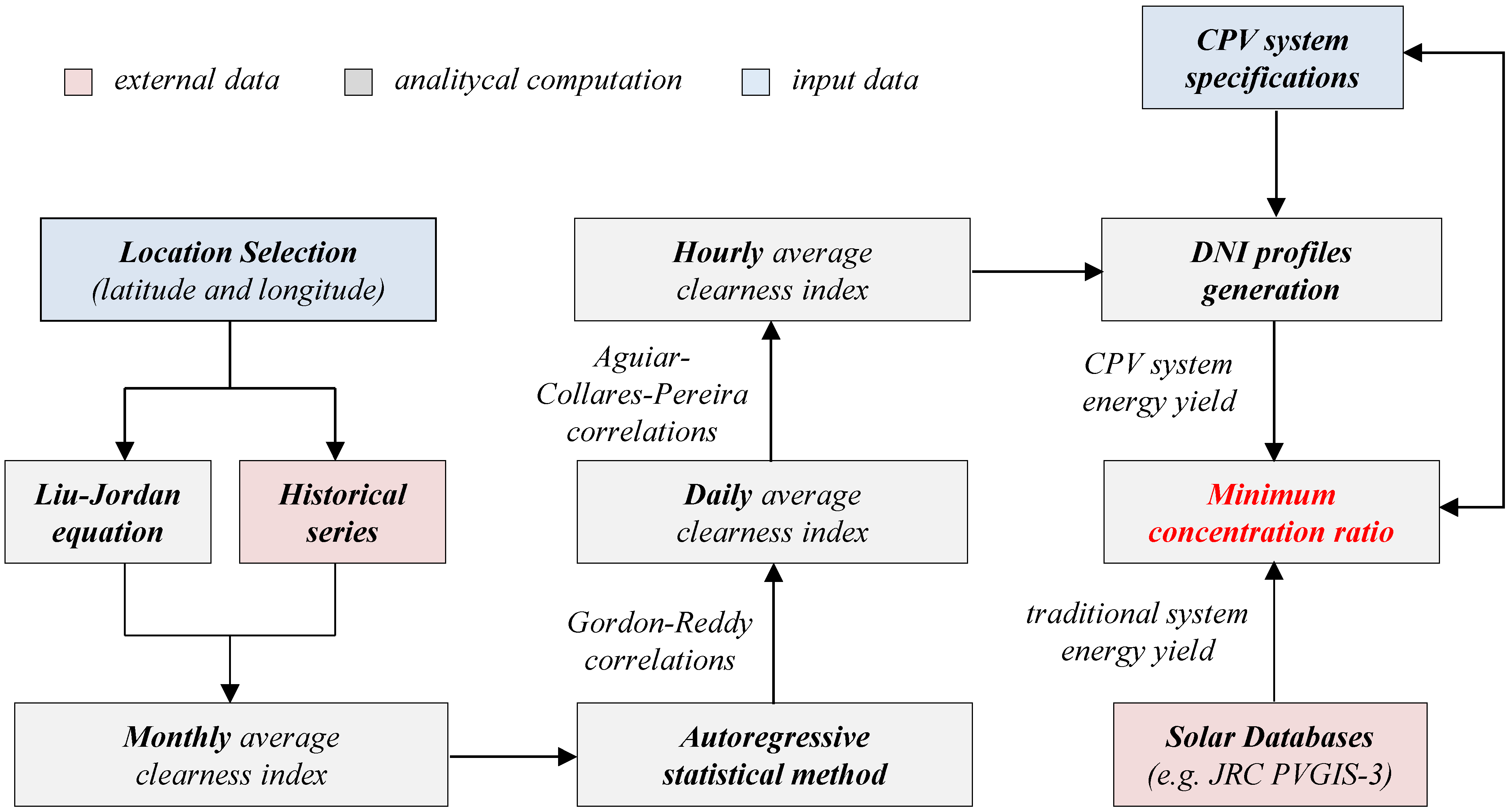
3.1. Solar Radiation

The solar radiation analysis incident on the terrestrial surface depends on astronomical angles (Table 1) that take into account the relative position between the Sun and the Earth.

Table 1. Astronomic angles and solar parameters [12].

Parameter	Symbol	Formula
Solar Declination	δ	$\text{δ}={\text{sin}}^{-1}\left[\text{sin}(23.45)·\text{sin}(360/365·(d-81))\right]$
Local Solar Time Meridian	LSTM	$LSTM=15°·∆T_{GMT}$ (for Italy $∆T_{GMT}=+1$)
Time Correction Factor	ΔT	$∆T=4·(longitude-LSTM)+EoT$
Equation of Time	EoT	$EoT=9.87·\text{sin}(2B)-7.53·\text{cos}(B)-1.5·\text{sin}(B)$
EoT Factor	B	$B=360°·(d-81)/365$
Local Time	LT	-
Local Solar Time	LST	$LST=LT+∆T/60-\left\{1h\right\}$
Solar Hour Angle	ω	$\text{ω}=15°·(LST-12)$
Solar Altitude	α	$\text{α}={\text{sin}}^{-1}\left[\text{sin}(\text{δ})·\text{sin}(\text{φ})+\text{cos}(\text{δ})·\text{cos}(\text{φ})·\text{cos}(\text{ω})\right]$
Zenith Angle	ϑz	${\vartheta }_{\text{z}}=90°-\text{α}$
Solar Azimuth	γ	$\text{γ}=\left\{\begin{array}{c}180°-{\text{cos}}^{-1}\left(\frac{\text{sin}(\text{α}) ·\text{sin}(\text{φ})-\text{sin}(\text{δ})}{\text{cos}(\text{α})·\text{cos}(\text{φ})}\right) \text{if} \text{ω}\le 0 \\ 180°+{\text{cos}}^{-1}\left(\frac{\text{sin}(\text{α}) ·\text{sin}(\text{φ})-\text{sin}(\text{δ})}{\text{cos}(\text{α})·\text{cos}(\text{φ})}\right) \text{if} \omega >0 \end{array}\right\}$

Table 1. Astronomic angles and solar parameters [12].

Parameter	Symbol	Formula
Solar Declination	δ	$\text{δ}={\text{sin}}^{-1}\left[\text{sin}(23.45)·\text{sin}(360/365·(d-81))\right]$
Local Solar Time Meridian	LSTM	$LSTM=15°·∆T_{GMT}$ (for Italy $∆T_{GMT}=+1$)
Time Correction Factor	ΔT	$∆T=4·(longitude-LSTM)+EoT$
Equation of Time	EoT	$EoT=9.87·\text{sin}(2B)-7.53·\text{cos}(B)-1.5·\text{sin}(B)$
EoT Factor	B	$B=360°·(d-81)/365$
Local Time	LT	-
Local Solar Time	LST	$LST=LT+∆T/60-\left\{1h\right\}$
Solar Hour Angle	ω	$\text{ω}=15°·(LST-12)$
Solar Altitude	α	$\text{α}={\text{sin}}^{-1}\left[\text{sin}(\text{δ})·\text{sin}(\text{φ})+\text{cos}(\text{δ})·\text{cos}(\text{φ})·\text{cos}(\text{ω})\right]$
Zenith Angle	ϑz	${\vartheta }_{\text{z}}=90°-\text{α}$
Solar Azimuth	γ	$\text{γ}=\left\{\begin{array}{c}180°-{\text{cos}}^{-1}\left(\frac{\text{sin}(\text{α}) ·\text{sin}(\text{φ})-\text{sin}(\text{δ})}{\text{cos}(\text{α})·\text{cos}(\text{φ})}\right) \text{if} \text{ω}\le 0 \\ 180°+{\text{cos}}^{-1}\left(\frac{\text{sin}(\text{α}) ·\text{sin}(\text{φ})-\text{sin}(\text{δ})}{\text{cos}(\text{α})·\text{cos}(\text{φ})}\right) \text{if} \omega >0 \end{array}\right\}$

The extraterrestrial solar radiation can be theoretically calculated for each day of the year by means of the following equation [13]:

$${\text{G}}_{\text{ext}}={\text{G}}_{\mathrm{c}}·\left[1+0.033·\text{cos}\left(\frac{360·\text{d}}{365}\right)\right]$$

(1)

where G_c is the solar constant, equal to 1367 W/m², and d is the number of days from the beginning of the year.

The global solar radiation can be evaluated by means of the following balance equation:

$${\text{G}}_{\text{tot}}={\text{ G}}_{\text{dir}}+{\text{G}}_{\text{dif}}+{\text{G}}_{\text{ref}}$$

(2)

where the global solar radiation is the sum of the direct, diffuse and reflected components. Multi-junction cells can only convert the direct solar radiation into electricity. The system orientation and installation site knowledge allows to calculate the direct solar radiation through empirical cloudless models based on the historical series of the solar irradiance data [14]:

$${\text{G}}_{\text{dir}}={\text{C}}_{\mathrm{n}} ·\text{A} · {\text{e}}^{-\left(\frac{\text{p}}{{\text{p}}_0}\right)·\frac{\text{B}}{\text{cos}({\text{θ}}_{\text{z}})}}$$

(3)

where C_n is the clearness number, a dimensionless factor which varies between 0.85 and 1.15; it takes into account the amount of water vapor and aerosol particles. The other parameters of Equation (3) are: solar zenith angle (θ_z), site pressure (p), standard pressure at 1 atm (p₀), empirical factors A and B which model the solar radiation amount that passes through the atmosphere and the diffuse radiation proportion [14].

A detailed analysis of the solar radiation requires the study of the actual climatic conditions. This can be carried out by means of non-cloudless models. In this paper, a statistical autoregressive model has been used [15]. A normal variable Z_d, representative of a random process which may be the succession of daily climatic conditions in a specific site, is introduced as a linear function of the same variable, referring to its previous states, plus an error term representing the statistical noise. This can be expressed as:

$${\text{Z}}_{\mathrm{d}}={\text{τ}}_1 · {\text{Z}}_{\text{d}-1}+{\text{τ}}_2 · {\text{Z}}_{\text{d}-2}+\dots +{\text{τ}}_{\mathrm{n}} · {\text{Z}}_{\text{d}-\text{n}}+{\text{r}}_{\mathrm{d}}$$

(4)

where τ_i are the autocorrelation coefficients. The analysis of historical series shows that it is possible to consider only the first order term. Furthermore, the first order autocorrelation coefficient, which varies between 0 to 0.6 depending on the site, can be reasonably approximated to 0.3 [15]. The statistical noise is a normal random variable which is defined from a sequence of random numbers z ∈ [0,1] having the following formulation:

$${\text{r}}_{\mathrm{d}}=\text{ σ}·[{\text{z}}^{0.135}-{(1-\text{z})}^{0.135}]/0.1975$$

(5)

Initializing Z₀ = 0, it is possible to generate a values series which approximates the climatic data historical series. The procedure is based on Gordon-Reddy method [16] which consists of empirical formulations expressed as a function of the average monthly clearness index (k_tm). This parameter is the ratio of the terrestrial solar energy on a horizontal surface (H_h) and the extraterrestrial solar energy (H_h0):

$${\text{k}}_{\text{tm}}=\frac{{\text{H}}_{\text{h}}}{{\text{H}}_{\text{h}0}}$$

(6)

The H_h value can be obtained by means of climatic databases [17], while monthly solar horizontal radiation H_h0 can be analytically calculated by Liu-Jordan formula [18]:

$${\text{H}}_{\text{h}0}=\frac{24{\text{ G}}_{\text{c}}}{\text{π}}·\left[1+0.033\text{cos}\left(\frac{360\text{d}}{365}\right)\right] ·\left[\text{cos}(\text{φ}) · \text{cos}(\text{δ}) · \text{sin}({\text{ω}}_{\text{s}})+\frac{2{\text{π ω}}_{\text{s}}}{360} · \text{sin}(\text{φ}) · \text{sin}(\text{δ})\right]$$

(7)

where ω_s is the sunset hour angle, defined as:

$${\text{ω}}_{\mathrm{s}}={\text{cos}}^{-1}\left[-\text{tan}(\text{φ}) · \text{tan}(\text{δ})\right]$$

(8)

The probability density function of the average daily clearness index is described by the following equation [16]:

$$\text{P}\left({\text{X}}_{\text{d}}\right)=\text{A} · {\text{X}}_{\mathrm{d}}^{\mathrm{n}} · \left(1-\frac{{\text{X}}_{\text{d}}}{{\text{X}}_{\text{max}}}\right)$$

(9)

The Gordon-Reddy coefficients are reported in Table 2. Equating the cumulative distribution functions of X_d and Z_d, an implicit equation is obtained; this must be solved iteratively:

$$\text{A} · {\text{X}}_{\mathrm{d}}^{\text{n}+1}=\raisebox{1ex}{$\text{F}\left({\text{Z}}_{\text{d}}\right)$}\!\left/ \!\raisebox{-1ex}{$\left(\frac{1}{\text{n}+1}-\frac{{\text{X}}_{\text{d}}}{\left(\text{n}+2\right) · {\text{X}}_{\text{max}}}\right)$}\right.$$

(10)

Solving Equation (10) in X_d, it is possible to generate a value for the average daily clearness index, considering that: ${\text{k}}_{\text{td}}={\text{X}}_{\mathrm{d}}·{\text{k}}_{\text{tm}}$.

Table 2. Gordon-Reddy coefficients.

Symbol	Formula
${\text{σ}}_{xd}^2$	$\left\{\begin{array}{c}0.1926 if \overline{k_{tm}}\le 0.2\\ \text{max}[0.01, (0.269-0.382·\overline{k_{tm}} ] if \overline{k_{tm}}>0.2\end{array}\right\}$
n	$-2.5+0.5\sqrt{9+8/{\text{σ}}_{xd}^2}$
Xmax	$(n+3)/(n+1)$
A	$\left(n+1\right)·\frac{(n+2)}{{\left(X_{\text{max}}\right)}^{n+1}}$

Table 2. Gordon-Reddy coefficients.

Symbol	Formula
${\text{σ}}_{xd}^2$	$\left\{\begin{array}{c}0.1926 if \overline{k_{tm}}\le 0.2\\ \text{max}[0.01, (0.269-0.382·\overline{k_{tm}} ] if \overline{k_{tm}}>0.2\end{array}\right\}$
n	$-2.5+0.5\sqrt{9+8/{\text{σ}}_{xd}^2}$
Xmax	$(n+3)/(n+1)$
A	$\left(n+1\right)·\frac{(n+2)}{{\left(X_{\text{max}}\right)}^{n+1}}$

Iterating this method during the year, it is possible to get a statistical profile of the horizontal solar radiation for a given site (Figure 2).

Figure 2. An example of daily solar irradiance profile generated for the city of Salerno (40.7°N–14.8°E) adopting the Gordon-Reddy statistical model.

Figure 2. An example of daily solar irradiance profile generated for the city of Salerno (40.7°N–14.8°E) adopting the Gordon-Reddy statistical model.

Table 3. Annual horizontal global irradiation comparison for different Italian sites.

Location	Solar atlas [19]	CM-SAF [20]	Model
Bari (41.1°N–16.9°E)	1625–1700 kWh/m2	1680 kWh/m2	1745 kWh/m2
Catania (37.5°N–15.1°E)	1775–1850 kWh/m2	1830 kWh/m2	1780 kWh/m2
Florence (43.8°N–11.2°E)	1475–1550 kWh/m2	1500 kWh/m2	1560 kWh/m2
Genova (44.4°N–9.0°E)	1400–1475 kWh/m2	1475 kWh/m2	1495 kWh/m2
Milan (45.5°N–9.2°E)	1325–1400 kWh/m2	1450 kWh/m2	1395 kWh/m2
Naples (41.1°N–14.3°E)	1625–1700 kWh/m2	1690 kWh/m2	1665 kWh/m2
Palermo (38.1°N–13.4°E)	1700–1775 kWh/m2	1790 kWh/m2	1740 kWh/m2
Rome (41.9°N–12.5°E)	1550–1625 kWh/m2	1670 kWh/m2	1625 kWh/m2
Turin (45.1°N–7.7°E)	1400–1475 kWh/m2	1460 kWh/m2	1425 kWh/m2

Table 3. Annual horizontal global irradiation comparison for different Italian sites.

Location	Solar atlas [19]	CM-SAF [20]	Model
Bari (41.1°N–16.9°E)	1625–1700 kWh/m2	1680 kWh/m2	1745 kWh/m2
Catania (37.5°N–15.1°E)	1775–1850 kWh/m2	1830 kWh/m2	1780 kWh/m2
Florence (43.8°N–11.2°E)	1475–1550 kWh/m2	1500 kWh/m2	1560 kWh/m2
Genova (44.4°N–9.0°E)	1400–1475 kWh/m2	1475 kWh/m2	1495 kWh/m2
Milan (45.5°N–9.2°E)	1325–1400 kWh/m2	1450 kWh/m2	1395 kWh/m2
Naples (41.1°N–14.3°E)	1625–1700 kWh/m2	1690 kWh/m2	1665 kWh/m2
Palermo (38.1°N–13.4°E)	1700–1775 kWh/m2	1790 kWh/m2	1740 kWh/m2
Rome (41.9°N–12.5°E)	1550–1625 kWh/m2	1670 kWh/m2	1625 kWh/m2
Turin (45.1°N–7.7°E)	1400–1475 kWh/m2	1460 kWh/m2	1425 kWh/m2

The annual horizontal solar radiation values have been obtained and compared to the data reported in solar radiation atlas [19] and in the CM-SAF PVGIS database [20] for different Italian cities (Table 3). The values obtained by the model are the arithmetic average calculated through the generation of 1000 irradiation profiles. The first-order autoregressive procedure is similarly used for the hourly clearness index (k_th). In this case empirical correlations by [21] are taken into account to generate a statistical profile of hourly weather conditions. Hourly clearness index is the input parameter for the direct, diffuse and reflected radiation evaluation. Considering the Equation (2) and characterizing it for each solar component, the complete balance equation is [15]:

$${\text{G}}_{\text{tot},\text{h}}={\text{ G}}_{\text{dir},\text{h}}·\frac{\text{cos}(\text{θ})}{\text{cos}({\text{θ}}_{\text{z}})}+{\text{G}}_{\text{dif},\text{h}} · \frac{1+\text{cos}(\text{β})}{2}+{\text{G}}_{\mathrm{h}} ·\text{ρ}·\frac{1-\text{cos}(\text{β})}{2}$$

(11)

where G_tot,h is the global horizontal radiation:

$${\text{G}}_{\text{tot},\text{h}}={\text{ G}}_{\text{c}}·\frac{{\text{ K}}_{\text{th}}}{\text{cos}({\text{θ}}_{\text{z}})}$$

(12)

β is the module tilt angle respect to the horizontal plane, ρ is the ground albedo and Gh is defined as the sum of horizontal direct and diffuse radiation: ${\text{G}}_{\mathrm{h}}={\text{ G}}_{\text{dir},\text{h}}+{\text{G}}_{\text{dif},\text{h}}$.

The Erbs predictive model [22] is used to quantify the radiation diffuse component on the horizontal surface. Hence, it is possible to determine the G_dir,h and the DNI on the module surface by means of the following expression:

$${\text{G}}_{\text{DNI}}={\text{ G}}_{\text{dir},\text{h}} · \left[\frac{\text{cos}\left(\text{α}\right)·\sin \left(\text{β}\right)·\text{cos}\left({\text{γ}}_{\text{s}}-\text{γ}\right)+\text{sin}\left(\text{α}\right)·\text{cos}\left(\text{β}\right)}{\text{cos}({\text{θ}}_{\text{z}})}\right]$$

(13)

where γ_s and γ are the azimuth of the direction to which the system is oriented, usually south in the northern hemisphere, and the solar azimuth respectively.

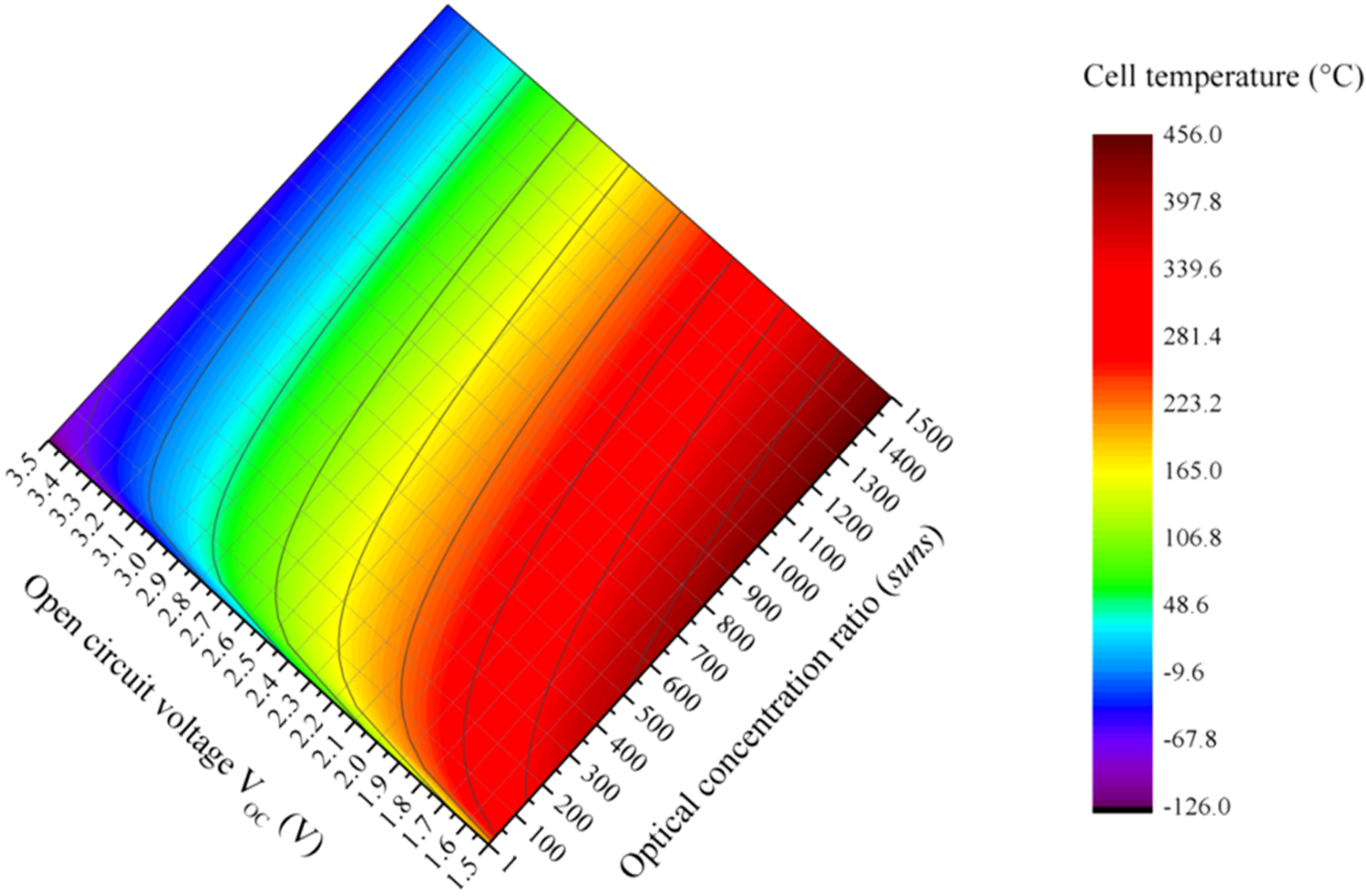
3.2. Solar Cell Electric Model

The single-junction photovoltaic cell behavior can be analyzed by means of the equivalent circuit model. From the electric point of view, an ideal cell is a current generator with a diode placed in parallel. To consider the effect of the internal dissipations, two resistances in series (R_s) and in parallel (R_sh, shunt resistance) are introduced.

The cell is described from the analytical point of view by the Shockley diode equation:

$$\text{I}={\text{I}}_{\text{L}}-{\text{I}}_{\mathrm{O}}·\left[{\text{e}}^{\frac{\text{q}\left(\text{V}+{\text{IR}}_{\text{s}}\right)}{\text{nkT}}}-1\right]-\frac{\text{V}+{\text{IR}}_{\text{s}}}{{\text{R}}_{\text{sh}}}$$

(14)

where I_L is the photo-generated current intensity, proportional to the incident solar radiation, I_O is the reverse saturation current intensity proportional to the p-n junction area, T is the absolute temperature, q is the elementary charge, k is the Boltzmann’s constant and n is the diode ideality factor, which varies between 1 and 2 in Si-based solar cells.

Equation (14) provides an accurate representation of the cell behaviour, although it cannot be directly applied because of the difficulty in the constitutive parameters determination. In practical applications, a simplified approach is adopted considering the following assumptions: uniform generation in cells subjected to the same operating conditions, negligible voltage drop in metallic conductors, negligible resistive effects and photo-generated current approximated to short-circuit current. Generally, the solar cells modeling is realized under open circuit and short circuit conditions. The open circuit voltage (V_OC) can be approximated to:

$${\text{V}}_{\text{OC}}\approx \frac{\text{nkT}}{\text{q}} · \text{ln}\left(\frac{{\text{I}}_{\text{L}}}{{\text{I}}_{\text{O}}}+1\right)$$

(15)

Considering a short circuit condition (V = 0) and high quality cells (low Rs and high Rsh), the following short circuit current expression is obtainable from Equation (14): ${\text{I}}_{\text{SC}}\approx {\text{I}}_{\mathrm{L}}$.

The previous equations are related to a solar cell under non-concentrated light. The effect of solar concentration occurs by means of the proportional increase of short circuit current intensity. The concentration ratio can be expressed in electric terms as follows:

$$\text{C}=\frac{{\text{I}}_{\text{SC}}}{{\text{I}}_{\text{SC},\text{r}}}$$

(16)

where I_SC,r indicates the short circuit current intensity without concentration. The expression of the open circuit voltage thus becomes:

$${\text{V}}_{\text{OC}}({\text{T}}_{\mathrm{r}},\text{C})\approx \frac{{\text{nkT}}_{\text{r}}}{\text{q}}· \text{ln}\left(\frac{{\text{I}}_{\text{L}}}{{\text{I}}_{\text{O}}}+1\right)\approx \frac{{\text{nkT}}_{\text{r}}}{\text{q}}· \text{ln}\left(\frac{{\text{I}}_{\text{SC}}}{{\text{I}}_{\text{O}}}\right)={\text{V}}_{\text{OC}}({\text{T}}_{\mathrm{r}},1)+\frac{{\text{nkT}}_{\text{r}}}{\text{q}}· \text{ln}\left(\text{C}\right)$$

(17)

This is the starting point to obtain the cell temperature under concentrated light. A first approach for multi-junction cells is the King’s model [23]:

$${\text{T}}_{\mathrm{c}}=\raisebox{1ex}{$\left({\text{V}}_{\text{OC}}-{\text{V}}_{\text{OC},\text{r}}+{\text{β}}_{\text{Voc}}\left(\text{C}\right)·{\text{T}}_{\text{r}}\right)$}\!\left/ \!\raisebox{-1ex}{$\left[\frac{\text{nk}}{\text{q}}·\text{ln}\left(\frac{{\text{I}}_{\text{SC}}}{{\text{I}}_{\text{SC},\text{r}}}\right)+{\text{β}}_{\text{Voc}}(\text{C})\right]$}\right.$$

(18)

where the subscript r indicates the parameters calculated in the reference conditions without concentration and β_Voc(C) is the open circuit temperature coefficient. The method used in this paper is based on the Xing Ju et al. model [24]. Hence, the multi-junction cell temperature is equal to:

$${\text{T}}_{\mathrm{c}}={\text{T}}_{\mathrm{r}}+\frac{\left[{\text{V}}_{\text{OC}}\left({\text{T}}_{\text{c}},\text{C}\right)-{\text{V}}_{\text{OC}}\left({\text{T}}_{\text{r}},1\right)-\frac{{\text{nkT}}_{\text{r}}}{\text{q}}·\ln \left(\text{C}\right)\right]}{{\text{β}}_{\text{Voc}}(\text{C})}$$

(19)

Using Spectrolab C1MJ cells (Spectrolab Inc., CA, USA), it is possible to estimate the analytical expression of the electrical parameters:

$${\text{β}}_{\text{Voc}}\left(\text{C}\right)=-6.4 ·{10}^{-3}+3.2143 ·{10}^{-4}·\text{ln}\left(\text{C}\right)$$

(20)

The data sheets analysis shows an ideality factor of 3.72 and a V_OC value in standard conditions of 2.54 V (Figure 3).

The multi-junction cell temperature profile can be determined corresponding to Maximum Power Point (MPP). In this case V_OC depends on the concentration ratio and the working temperature. By means of the data sheets interpolations the following expression has been obtained:

$${\text{V}}_{\text{ MPP}}=-1.285 · {10}^{-12} · {\text{C}}^4+3.380 · {10}^{-9} · {\text{C}}^3-3.264 · {10}^{-6} · {\text{C}}^2+1.253 · {10}^{-3} · \text{C}+2.543$$

(21)

where the numerical coefficients are calculated in standard conditions. Substituting Equation (21) in Equation (19) the cell temperature can be determined:

$${\text{T}}_{\text{MPP}}={\text{T}}_{\mathrm{r}}+\left[\frac{{\text{V}}_{\text{ MPP}}-2.543-3.2143 · {10}^{-4} · 298.15·\text{ln}\left(\text{C}\right)}{-6.4·{10}^{-3}+3.2143 · {10}^{-4} · \text{ln}\left(\text{C}\right)}\right]$$

(22)

In order to determine the cell temperature, it has been necessary to assume that the inverter instantaneously imposes a specific electric voltage profile to the cell. Although it is not possible to achieve MPP in open circuit conditions, a voltage profile must be imposed in order to build an analytical model of multi-junction cell temperature; the voltage profile closer to the one requested is the V_MPP profile, calculated empirically through Equation (21). This assumption has been confirmed by the correspondence between the resulting temperature profile (Figure 4) and the experimental indications given by CPV systems manufacturers corresponding to the maximum operating temperature (110–120 °C) under high solar irradiance conditions.

Figure 3. Multi-junction cell temperature as function of V_oc and C.

Figure 3. Multi-junction cell temperature as function of V_oc and C.

Figure 4. Multi-junction cell temperature at MPP as function of optical concentration ratio in standard conditions.

Figure 4. Multi-junction cell temperature at MPP as function of optical concentration ratio in standard conditions.

In Figure 4 concentration ratio is expressed in suns (1 sun = 1000 W/m²) but the solar direct irradiance in real applications is generally lower than 1000 W/m² and this implies a lower real level of concentration, justifying thus the theoretical limit reported by cells manufacturers.

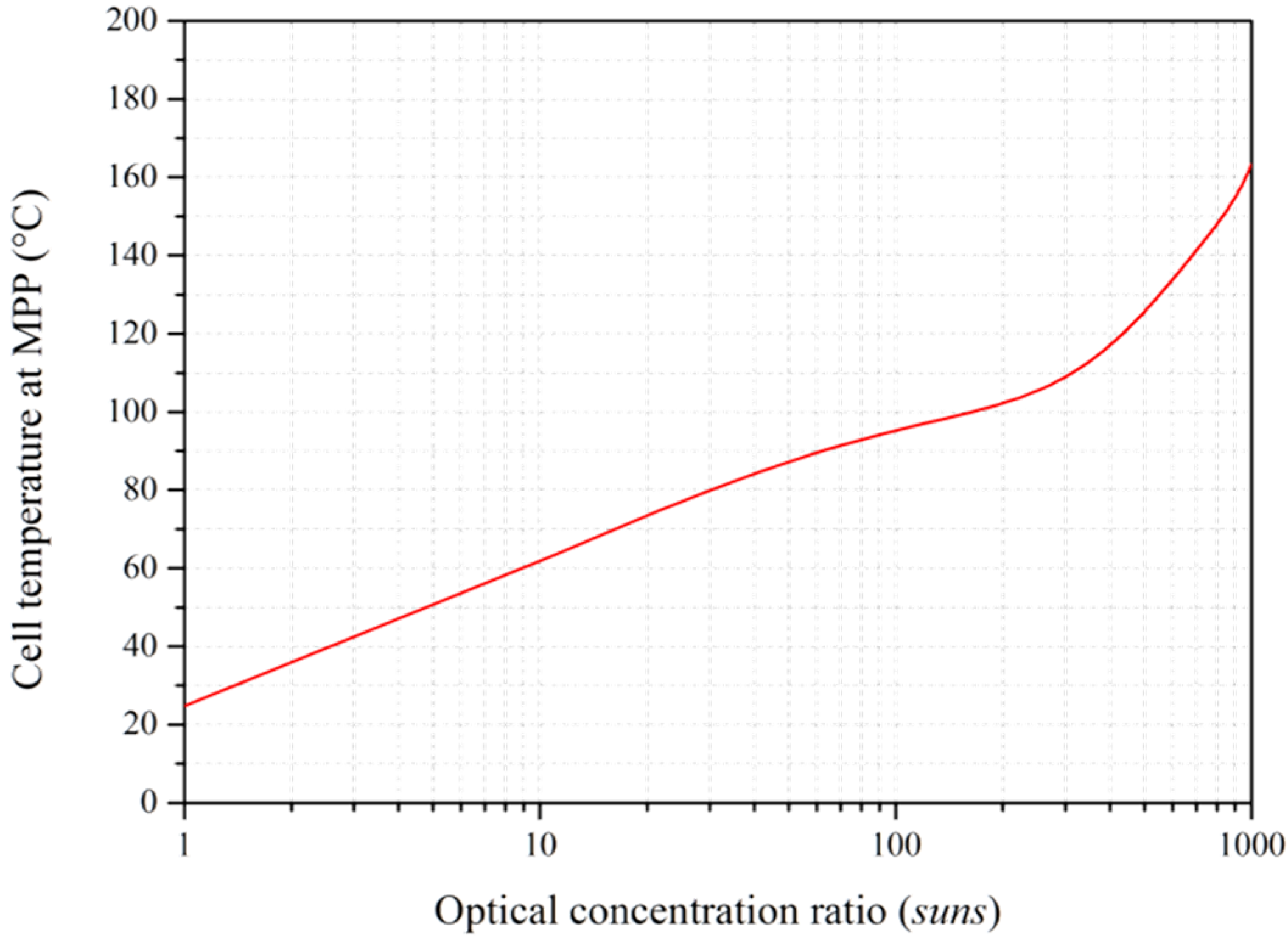
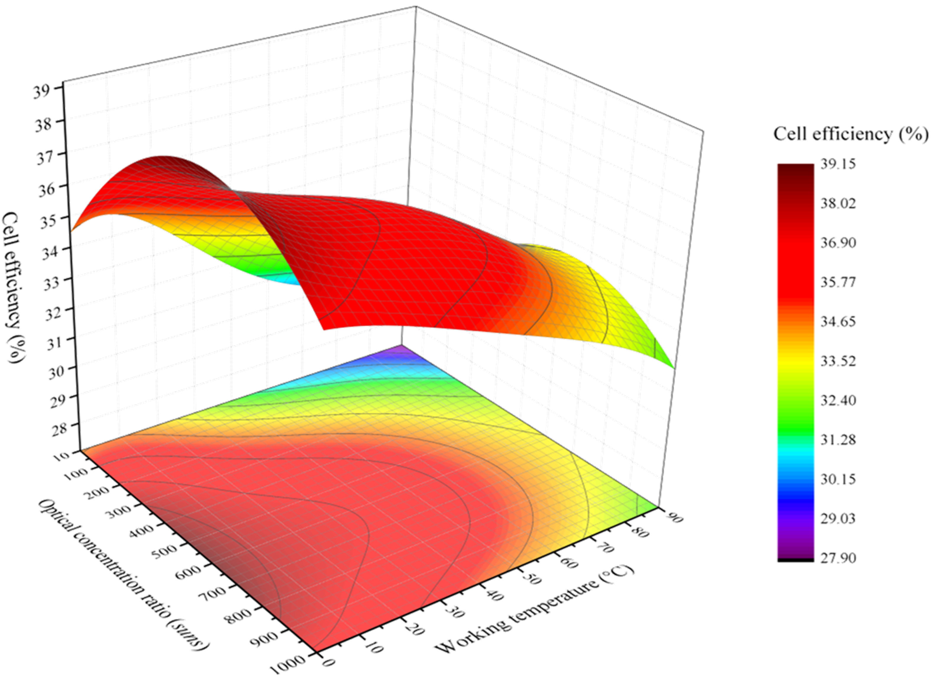
3.3. Cell Efficiency

The cell efficiency depends on the working temperature T_w and the concentration ratio C. By means of a double interpolation of C1MJ data sheets, it is possible to empirically estimate the cell efficiency as (Figure 5):

$$\text{η}({\text{T}}_w,\text{C})=\text{a}\left({\text{T}}_w\right) · {\text{C}}^2+\text{b}\left({\text{T}}_w\right)·\text{C}+\text{c}({\text{T}}_w)$$

(23)

where a(T), b(T) and c(T) coefficients are equal to:

$$\text{a}\left({\text{T}}_w\right)=-3.45 · {10}^{-12} · {{\text{T}}_w}^4+6.61 · {10}^{-10} · {{\text{T}}_w}^3-4.07 · {10}^{-8} · {{\text{T}}_w}^2+8.27 · {10}^{-7} · {\text{T}}_w-1.40 · {10}^{-5}$$

Figure 5. Electric efficiency profile of a multi-junction cell.

Figure 5. Electric efficiency profile of a multi-junction cell.

3.4. Electric and Thermal Power

The CPV module electric power can be expressed as:

$${\text{P}}_{\text{el}}=\left[\text{n} · {\text{C}}_{\text{x}} · {\text{G}}_{\text{DNI}} ·\text{ η}\left(\text{T},\text{C}\right) · {\text{η}}_{\text{opt}}\left({\text{C}}_{\text{x}}\right) · {\text{η}}_{\text{tr}}-{\text{P}}_{\text{loss}}\right] · {\text{A}}_{\text{mod}} · {\text{η}}_{\text{inv}}$$

(24)

where n is the number of solar cells, A_mod is the active surface of the CPV module, C_x is the geometric concentration ratio, η_opt is the optical efficiency (0.65 ÷ 0.85), η_tr is the tracking system efficiency (generally > 0.95) and P_loss is the parasitic power due to the circulation pump and the solar tracker. This quantity is generally negligible if compared to the solar energy captured by means of the tracking system. In many cases the parasitic power is indeed less than 3% of the total incident solar power [25]. The inverter allows the conversion of direct current into alternating current, suitable for the network distribution. The inverter efficiency increases with the load and the power, reaching values even higher than 95%; a typical value of 90% is used in the model [26]. Theoretically, thermal power is the amount of direct solar radiation incident on the cell which is not converted into electricity:

$${\text{P}}_{\text{th}}=\left[\text{n} · {\text{C}}_{\text{x}} · {\text{G}}_{\text{DNI}} · {\text{η}}_{\text{opt}}\left({\text{C}}_{\text{x}}\right) · {\text{η}}_{\text{tr}}\right] · \left[1-\text{η}\left(\text{T},\text{C}\right)\right] · {\text{A}}_{\text{mod}}$$

(25)

Considering the technical specifications of some commercial solutions and experimental systems, the model validation has been performed (Table 4). The comparison has been realized using as reference CPV technologies of different size and type. The model flexibility and accuracy have been demonstrated by the small difference between calculated and nominal values (Table 4). The model values have been adjusted by considering technical specifications such as the efficiency (solar cell, optics, inverter, module assembly, etc.), the solar cells active area and other loss factors reported in the data sheets. The CPV/T systems enable the thermal energy recovery by means of a hydraulic circuit whose configuration can vary significantly; in particular, in this analysis the circuit reported in Figure 1b has been considered.

Table 4. CPV model validation.

System	Output power	Model	Δ
ArimaEco CPV G1 [a]	621 Wp	613.5 Wp	−1.2%
Meridian MGM16-96 [b]	96 Wp	97.9 Wp	+2.0%
Emcore G3-1090x [c]	455 Wp	457.8 Wp	+0.6%
GPW HCPV [d]	400 Wp	396.8 Wp	−0.8%
Mini Dish CPV [26]	172 Wp	171.3 Wp	−0.4%
Mini Dish CPV [26]	530 Wth	522.9 Wth	−1.3%

[a] Arima EcoEnergy technologies corp., Corso Garibaldi 40, Seveso (Italy); [b] Meridian Green Energy Int. Ltd., RM.3D, Cheng Yiu Building No.169 Castle Peak Road Tsuen Wan (Hong Kong); [c] Emcore corp., 10420 Research Rd. SE, Bldg. 1 Albuquerque, NM 87123 (USA); [d] GPW-African Green Dev. Ltd., 24 Smith Street, Bromhof, Randburg, 2154, Gauteng (South Africa).

Table 4. CPV model validation.

System	Output power	Model	Δ
ArimaEco CPV G1 [a]	621 Wp	613.5 Wp	−1.2%
Meridian MGM16-96 [b]	96 Wp	97.9 Wp	+2.0%
Emcore G3-1090x [c]	455 Wp	457.8 Wp	+0.6%
GPW HCPV [d]	400 Wp	396.8 Wp	−0.8%
Mini Dish CPV [26]	172 Wp	171.3 Wp	−0.4%
Mini Dish CPV [26]	530 Wth	522.9 Wth	−1.3%

[a] Arima EcoEnergy technologies corp., Corso Garibaldi 40, Seveso (Italy); [b] Meridian Green Energy Int. Ltd., RM.3D, Cheng Yiu Building No.169 Castle Peak Road Tsuen Wan (Hong Kong); [c] Emcore corp., 10420 Research Rd. SE, Bldg. 1 Albuquerque, NM 87123 (USA); [d] GPW-African Green Dev. Ltd., 24 Smith Street, Bromhof, Randburg, 2154, Gauteng (South Africa).

Convective and radiative thermal losses related both to the front and back part of the CPV/T module are considered negligible [5,26]. In particular, under the assumption of water circuit thermal insulation and vacuum inside the hermetically sealed CPV/T module, the convective exchange is negligible. Moreover, the radiative exchange, considering the small active surface of multi-junction cells (approximately 1 cm²), involves a negligible value (order of magnitude of 1–10 W) when compared with the typical values of the CPV/T systems thermal power, as shown in Table 4. Hence, there are neither significant convective losses nor radiative losses. In particular, it has been observed in [10] that the thermal losses related to the CPV/T system and calculated according to the equations reported in [26], are included between 1% and 3%.

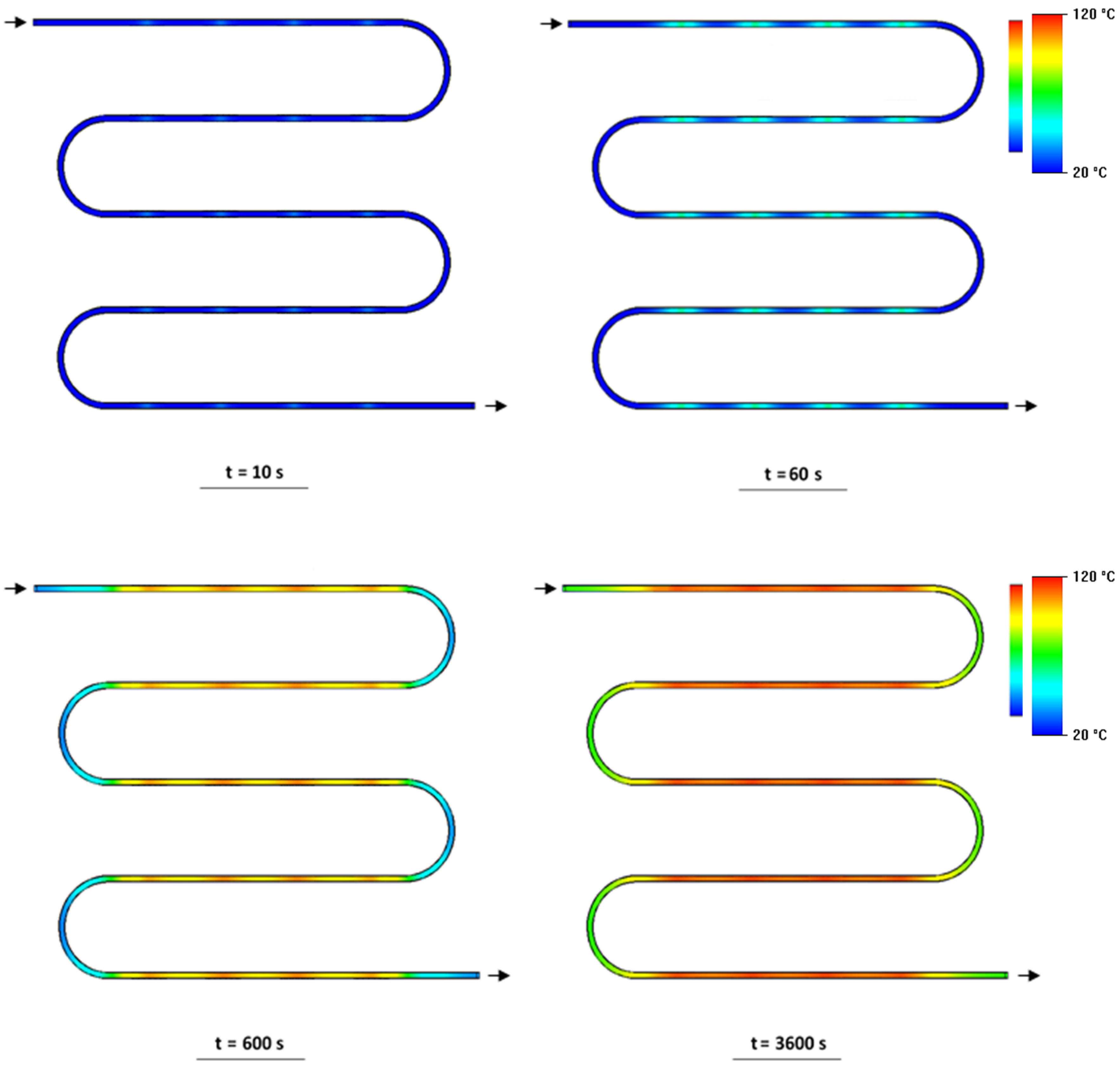
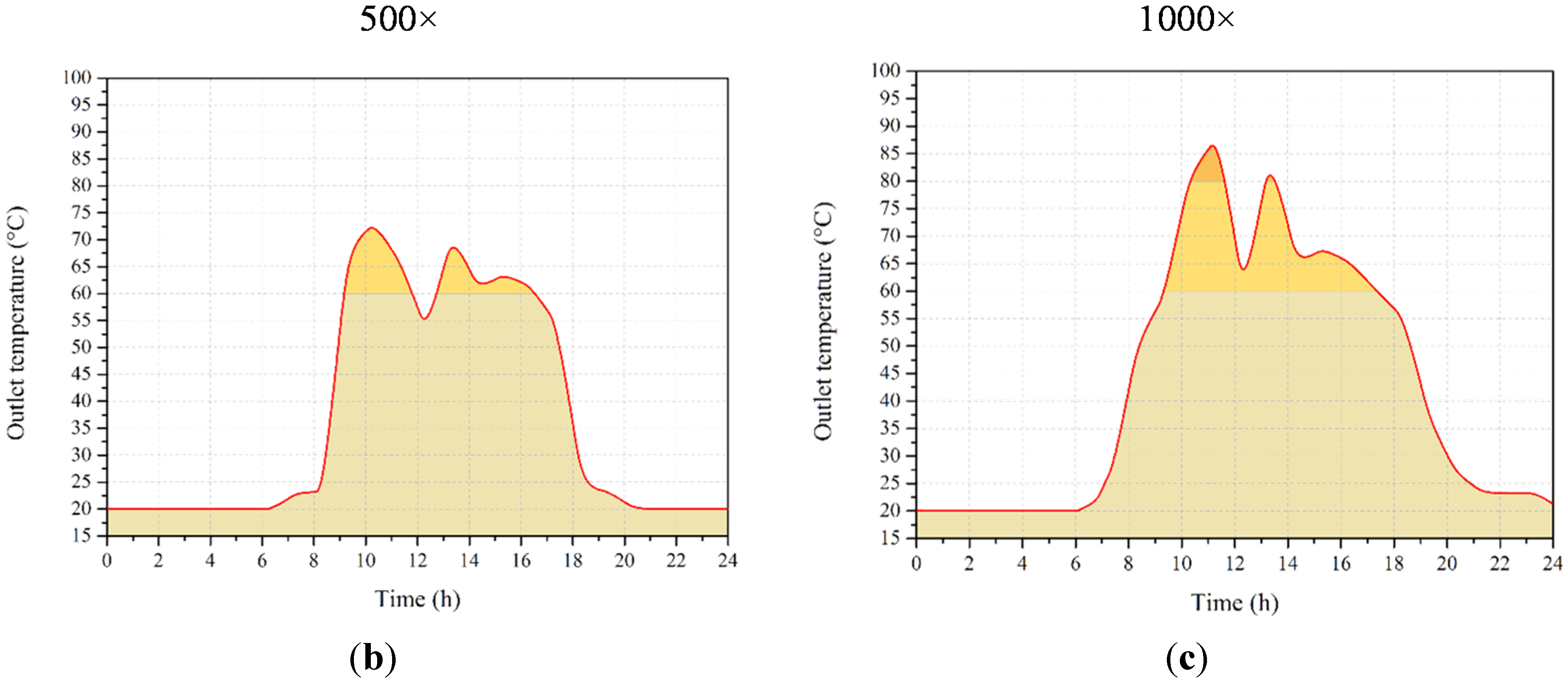
3.5. CPV/T System FEM Analysis

In order to take into account the CPV/T system structural complexity in terms of materials, geometries, heat exchange mechanisms and boundary conditions, an analytical approach is adopted to study the CPV/T system thermal transient; in particular, the Finite Element Method (FEM) is used. The FEM technique is based on the generation of discrete domains (mesh) where the numerical integration of the mass, momentum and energy balance equations is performed. This can be realized by means of a Computational Fluid Dynamics (CFD) simulation software; in this paper, Solidworks^® FlowSimulation tool has been used (Solidworks: Waltham, MA, USA, 2012). A three-dimensional graphical model of the analysis domain and of the CPV/T system components has been realized. Owing to the absence of constructive standards, the configuration of Figure 1 has been considered in the model as reference. The definition of initial and boundary conditions has allowed to initialize the FEM technique and to obtain the time trend of the refrigerant fluid temperature. This allows to evaluate the CPV/T system potentialities in trigenerative applications.

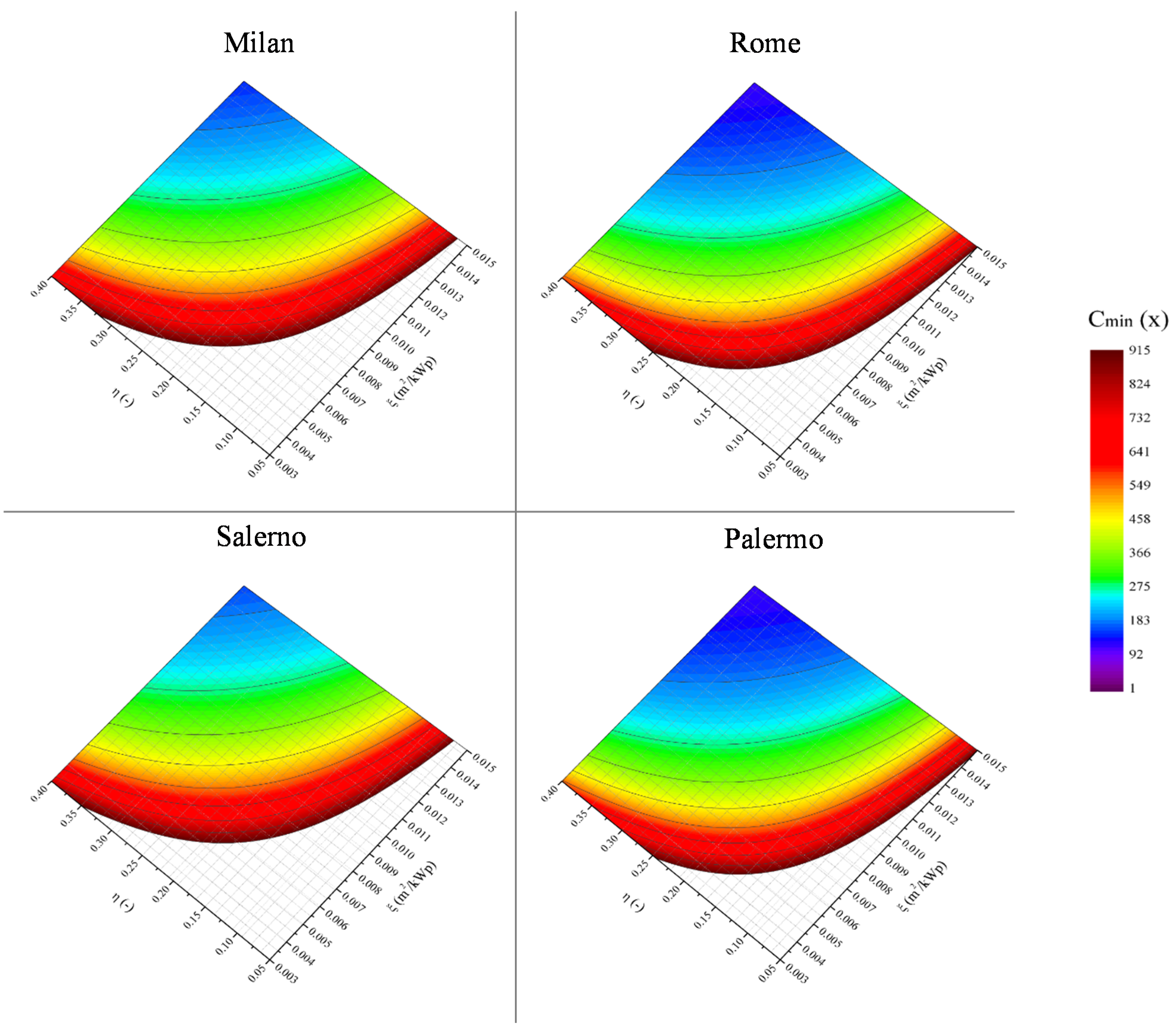
4. Energy and Economic Analysis

The CPV systems can convert a solar radiation amount that is substantially higher than silicon conventional systems thanks to optics and multi-junction cells. Although these cells are the most efficient photovoltaic technology, they can only convert into electricity the solar radiation direct component. Hence, it is essential to determine the convenience limit of CPV systems in comparison to mono-crystalline silicon systems. This can be realized estimating the electricity annual production. CM-SAF and PVGIS-3 models for traditional PV systems have been used [20]. Gordon-Reddy statistical model and UNI 10349 data [17] for the generation of DNI profile have been used. The average annual electricity yield per kW_p of a CPV system can be theoretically defined as:

$${\text{E}}_{\text{CPV}}=\text{C} · {\overline{\text{G}}}_{\text{DNI}} · {\text{η}}_{\text{tot}} · \text{t} · \text{ξ}=\text{C} · {\text{H}}_{\text{CPV}} · {\text{η}}_{\text{tot}} · \text{ξ}$$

(26)

where ${\overline{\text{G}}}_{\text{DNI}}$ is the average direct solar irradiance incident on the module surface in the reference time t, η_TOT is the system total efficiency (including the cell, optics, inverter efficiencies) while ξ is a factor that indicates the active surface per power unit. The energy produced by the CPV system will be compared with the traditional system performance E_TRD in order to determine the energy break-even point.

The procedure (Figure 6) calculates the clearness index based on the average insolation data. It is possible to generate an appropriate DNI profile by means of the Gordon-Reddy statistical model. Modules are supposed orthogonal to the direction of sunlight because this is the configuration adopted in the reference databases. The procedure is initialized with random numbers. Hence, there is a results variability representative of random climatic conditions. Therefore, it is essential to realize a multiple generation of DNI profiles considering average values. These will be then compared to the solar databases in order to determine the minimum concentration ratio (C_min) corresponding to which the CPV solution is energetically preferable. Equating traditional and CPV system the expected yield (Equation (26)), it is possible to express the energy break-even point in terms of concentration ratio using the following equation:

$${\text{C}}_{\text{min}}=\raisebox{1ex}{${\text{E}}_{\text{TRD}}$}\!\left/ \!\raisebox{-1ex}{$({\text{H}}_{\text{CPV}} · {\text{η}}_{\text{tot}} · \text{ξ})$}\right.$$

(27)

Fixed the CPV module, ξ and η_tot are known and C_min value is thus defined. If the geometric concentration ratio of the CPV system is inferior to C_min, traditional mono-crystalline solution should be preferred.

Figure 6. Flow chart of the energy convenience evaluation method.

Figure 6. Flow chart of the energy convenience evaluation method.

5. Results and Discussion

The CPV system use depends on its energy and economic convenience in comparison with a traditional power generation system. In particular, the convenience profile for a generic CPV system in terms of C_min has been obtained adopting an energy evaluation method. In Figure 7a wider colored area implies a greater number of combinations efficiency-active surface and then a higher application possibility. A wider blank area, non-convenience area, or alternatively larger red bands indicate higher levels of the required concentration. Hence, sites with a lower annual solar radiation such as Milan (North Italy) are disadvantaged compared to sites with higher solar radiation, such as Palermo (South Italy). The CPV systems configuration can vary significantly and as consequence installation, management and maintenance costs change.

Using the economic evaluation method by King et al. [27], it is possible to determine the economic convenience break-even point of concentrating photovoltaic systems compared to traditional energy generation systems. The global capital costs have been divided into photovoltaic costs (cells, lenses, module cables, etc.), BOS costs (auxiliary structures, installation, operation, maintenance and financing) and inverter cost. Considering the DNI values of a specific site and the estimated CPV costs [27], it is possible to determine for a selected system the simple payback period (Figure 8). For a medium concentration module, the payback varies between 5 and 8 years. These values are congruent with the specifications of small-scale commercial systems (Sahaj Solar Power Inc. Ltd., Gujarat, India) and large-scale solar installations [28,29], and they increase when a CPV/T system is considered [11].

Figure 7. Minimum concentration ratio (C_min) in several Italian sites calculated by means of the energy convenience evaluation method.

Figure 7. Minimum concentration ratio (C_min) in several Italian sites calculated by means of the energy convenience evaluation method.

Once known the C_min value that allows to satisfy the user electric load, it is possible to evaluate by means of the FEM simulation the refrigerant fluid temperature obtainable by the CPV/T system in order to evaluate its application potential. The FEM allows to analyze the thermal exchange mechanism of a CPV/T module. A single module configuration with coil hydraulic circuit and with twenty triple-junction cells has been considered. FEM simulation has been performed in transient conditions, considering simultaneously conductive, convective and radiative thermal exchange. The simulation has been then initialized by setting the following working conditions: fluid inlet temperature (20 °C), diameter of heat recovery circuit (20 mm), fluid volumetric flow rate (0.2 m³/h). The simulation time interval has been set to 10 seconds in order to achieve the best compromise between the duration of the simulation process and the consistency of the thermal exchange analysis. Moreover, the thermal insulation hypothesis of the module pipes has been considered [5]. First of all the fluid temperature determination has been evaluated fixing the cell temperature at 120 °C that generally represents the maximum operating temperature. Hence, it has been possible to provide an indication of the maximum output temperature achievable by the thermal recovery circuit (Figure 9). Using Solidworks^® FlowSimulation the model has been divided into a mesh consisting of 137,729 elements for the solids parts and 10,391 for the fluid parts. The convergence has been reached after 1000 iterations, corresponding to a simulated physical time of 10,000 seconds (2h 46m 40s). After this time, the fluid outlet average temperature has been of 75.4 °C.

Figure 8. Payback time for several Italian sites calculated by means of the King’s method [29] for ArimaEco CPV G1 module.

Figure 8. Payback time for several Italian sites calculated by means of the King’s method [29] for ArimaEco CPV G1 module.

In real applications, the cell temperature depends instantly on the level of direct solar irradiance and therefore cannot be considered constant. On the contrary, it is possible to realize a DNI profile with statistical methods and to generate the related thermal profile of the cell; this represents the FEM simulation input. The method can be applied to each site whose information about climatic historical series is available. In Figure 10a a possible random profile for the city of Salerno is shown. The curve is statistically generated and is representative of a mainly sunny day with partial cloudiness during central hours. The analysis is related to two cases of medium (500×, Figure 10b) and high (1000×) concentration (Figure 10c). In this case, the operating limit of 120 °C has been removed to consider the potentialities of new generations multi-junction cells. The results analysis has allowed to observe that the fluid outlet temperature is on average about 10 °C higher when a HCPV module is adopted. It has been also possible to note that temperatures higher than 80 °C can be obtained under high irradiance conditions and this allows the solar cooling systems use during the summer months. Moreover, it is important to observe that considering a module with more cells, the time necessary to reach the required temperature decreases. All this demonstrates the possibility to couple a CPV/T system with an absorption chiller in solar cooling applications.

Figure 9. Fluid thermal profile with the cell temperature fixed at 120 °C.

Figure 9. Fluid thermal profile with the cell temperature fixed at 120 °C.

Figure 10. Fluid temperature trend of a CPV/T system subjected to (a) a random DNI profile simulated for the city of Salerno in case of C equal to (b) 500× and to (c) 1000×.

Figure 10. Fluid temperature trend of a CPV/T system subjected to (a) a random DNI profile simulated for the city of Salerno in case of C equal to (b) 500× and to (c) 1000×.

6. Conclusions

In this paper is a dynamic model of a CPV/T system has been studied and the FEM technique has been adopted. Triple-junction solar cells (GaInP/GaInAs/Ge) placed on a coil circuit where the refrigerant fluid flows have been considered. An accurate DNI profile generation method has been also considered by means of the Gordon-Reddy statistical approach. The results have been successfully tested by means of the comparison with solar atlas and insolation databases. The model has allowed to determine the cell temperature and efficiency, the electric and thermal powers of the CPV/T module and the refrigerant fluid outlet temperature. The fluid temperature has been evaluated corresponding both to a constant cell temperature equal to 120 °C and to a cell temperature variable with the DNI as occurs in the real applications. It has been important to evaluate the necessary C_min value in order to opportunely size the concentrating system according to the user electric load demand. Hence, an energy evaluation method has been introduced to determine the convenience profile of a generic CPV system in terms of C_min. Once known the C_min value, the fluid outlet temperature has been evaluated in the time by means of the FEM technique, and the possibility to use a CPV/T system in solar heating and cooling applications has been verified. In particular, it has been observed that temperatures higher than 80 °C are obtained in high irradiance conditions and this allows the solar cooling systems use during the summer months. Future developments will concern the dynamic model study of a CPV/T system adopted for a domestic user considering more modules with a variable number of cells in order to properly size the system, and to verify if the time necessary to reach the required temperature decreases and the thermal and cooling loads are satisfied.

References

1. Zahedi, A. Review of modeling details in relation to low-concentration solar concentrating photovoltaic. Renew. Sustain. Energy Rev. 2011, 15, 1609–1614. [Google Scholar] [CrossRef]
2. Chemisana, D. Building integrated concentrating photovoltaics: A review. Renew. Sustain. Energy Rev. 2010, 15, 603–611. [Google Scholar] [CrossRef]
3. Cotal, H.; Fetzer, C.; Boisvert, J.; Kinsey, G.; King, R.; Hebert, P.; Yoon, H.; Karam, N. III–V multi-junction solar cells for concentrating photovoltaics. Energy Environ. Sci. 2009, 2, 174–192. [Google Scholar] [CrossRef]
4. Li, M.; Ji, X.; Li, G.; Wei, S.; Li, Y.; Shi, F. Performance study of solar cell arrays based on a Trough Concentrating Photovoltaic/Thermal system. Appl. Energy 2011, 88, 3218–3227. [Google Scholar] [CrossRef]
5. Mittelman, G.; Kribus, A.; Dayan, A. Solar cooling with concentrating photovoltaic/thermal (CPVT) systems. Energy Convers. Manag. 2007, 48, 2481–2490. [Google Scholar] [CrossRef]
6. Kandilli, C. Performance analysis of a novel concentrating photovoltaic combined system. Energy Convers. Manag. 2013, 67, 186–196. [Google Scholar] [CrossRef]
7. Li, M.; Li, G.L.; Ji, X.; Yin, F.; Xua, L. The performance analysis of the trough concentrating solar photovoltaic/thermal system. Energy Convers. Manag. 2011, 52, 2378–2383. [Google Scholar] [CrossRef]
8. Kosmadakis, G.; Manolakos, D.; Papadakis, G. Simulation and economic analysis of a CPV/thermal system coupled with an organic Rankine cycle for increased power generation. Sol. Energy 2011, 85, 308–324. [Google Scholar] [CrossRef]
9. Al-Alili, A.; Hwang, Y.; Radermacher, R.; Kubo, I. A high efficiency solar air conditioner using concentrating photovoltaic/thermal collectors. Appl. Energy 2012, 93, 138–147. [Google Scholar] [CrossRef]
10. Renno, C.; Petito, F. Design and modeling of a concentrating photovoltaic thermal (CPV/T) system for a domestic application. Energy Build. 2013, 62, 392–402. [Google Scholar] [CrossRef]
11. Renno, C. Optimization of a concentrating photovoltaic thermal (CPV/T) system used for a domestic application. Appl. Therm. Eng. 2014, 67, 396–408. [Google Scholar] [CrossRef]
12. Honsberg, C.; Bowden, S. PVEducation.org-PVCDROM. Available online: http://www.pveducation.org/ (accessed on 9 June 2014).
13. Duffie, J.A.; Beckmann, W. Solar Engineering of Thermal Processes; John Wiley & Sons: New York, NY, USA, 2006. [Google Scholar]
14. Owen, M.S. ASHRAE Handbook: HVAC Applications; ASHRAE: Atlanta, GA, USA, 2011. [Google Scholar]
15. Eicker, U. Solar Technologies for Buildings; John Wiley & Sons: New York, NY, USA, 2003. [Google Scholar]
16. Gordon, J.M.; Reddy, T.A. Time series analysis of daily horizontal solar radiation. Sol. Energy 1988, 41, 215–226. [Google Scholar] [CrossRef]
17. Heating and Cooling of Buildings. Climatic Data; UNI 10349, UNI Italian Company: Milan, Italy, 1994.
18. Liu, B.Y.H.; Jordan, R.C. The interrelationship and characteristic distribution of direct, diffuse and total solar radiation. Sol. Energy 1960, 4, 1–19. [Google Scholar] [CrossRef]
19. SolarGIS. Available online: http://solargis.info/doc/free-solar-radiation-maps-GHI (accessed on 20 June 2014).
20. Photovoltaic Geographical Information System (PVGIS). Available online: http://re.jrc.ec.europa.eu/pvgis/ (accessed on 25 June 2014).
21. Aguiar, R.; Collares-Pereira, M. TAG: A time-dependent, autoregressive, Gaussian model for generating synthetic hourly radiation. Sol. Energy 1992, 49, 167–174. [Google Scholar] [CrossRef]
22. Erbs, D.G.; Klein, S.A.; Duffie, J.A. Estimation of the diffuse radiation fraction for hourly, daily and monthly-average global radiation. Sol. Energy 1982, 28, 293–302. [Google Scholar] [CrossRef]
23. King, R.R.; Law, D.C.; Edmondson, K.M.; Fetzer, C.M.; Kinsey, G.S.; Yoon, H.; Sherif, R.A.; Karam, N.H. 40%-efficient metamorphic GaInP/GaInAs/Ge multi-junction solar cells. Appl. Phys. Lett. 2007, 90, 183516. [Google Scholar] [CrossRef]
24. Ju, X.; Vossier, A.; Wang, Z.; Dollet, A.; Flamant, G. An improved temperature estimation method for solar cells operating at high concentrations. Sol. Energy 2013, 93, 80–89. [Google Scholar] [CrossRef]
25. Mousazadeh, H.; Keyhani, A.; Javadi, A.; Mobli, H.; Abrinia, K.; Sharifi, A. A review of principle and sun-tracking methods for maximizing solar systems output. Renew. Sustain. Energy Rev. 2009, 13, 1800–1818. [Google Scholar] [CrossRef]
26. Kribus, A.; Kaftori, D.; Mittelman, G.; Hirshfeld, A.; Flitsanov, Y.; Dayan, A. A miniature concentrating photovoltaic and thermal system. Energy Convers. Manag. 2006, 47, 3582–3590. [Google Scholar] [CrossRef]
27. King, R.R.; Bhusari, D.; Larrabee, D.; Liu, X.Q.; Rehder, E.; Edmondson, K.; Cotal, H.; Jones, R.K.; Ermer, J.H.; Fetzer, C.M.; et al. Solar cell generations over 40% efficiency, 26th EU PVSEC, Hamburg, Germany, 2011. Prog. Photovolt. 2012, 20, 801–815. [Google Scholar] [CrossRef]
28. Mastrullo, R.; Renno, C. A thermoeconomic model of a photovoltaic heat pump. Appl. Therm. Eng. 2010, 30, 1959–1966. [Google Scholar] [CrossRef]
29. Gómez-Gil, F.J.; Wang, X.; Barnett, A. Analysis and prediction of energy production in concentrating photovoltaic (CPV) installations. Energies 2012, 5, 770–789. [Google Scholar] [CrossRef]