Opportunities for Energy Crop Production Based on Subfield Scale Distribution of Profitability

Abstract
:1. Introduction
2. Methods
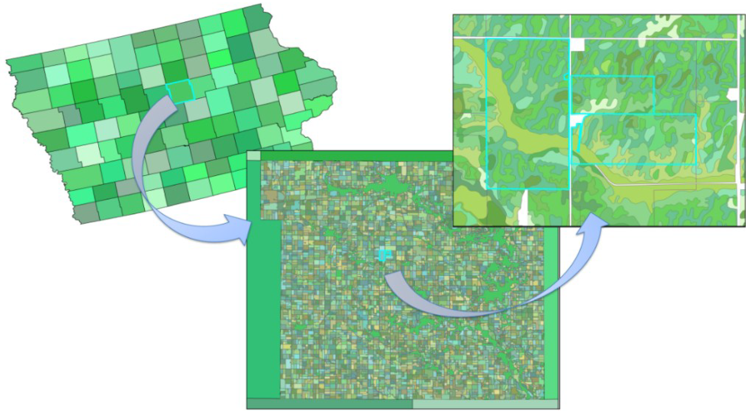
2.1. Study Area
2.2. Establishing Subfield Yields
2.3. Profit Calculation
2.4. Sustainable Stover Calculation
2.4.1. Climate Data
2.4.2. Crop Rotations
2.4.3. Land Management and Tillage Practices
2.4.4. Residue Removal Practices
2.5. Data Analysis
3. Results and Discussion
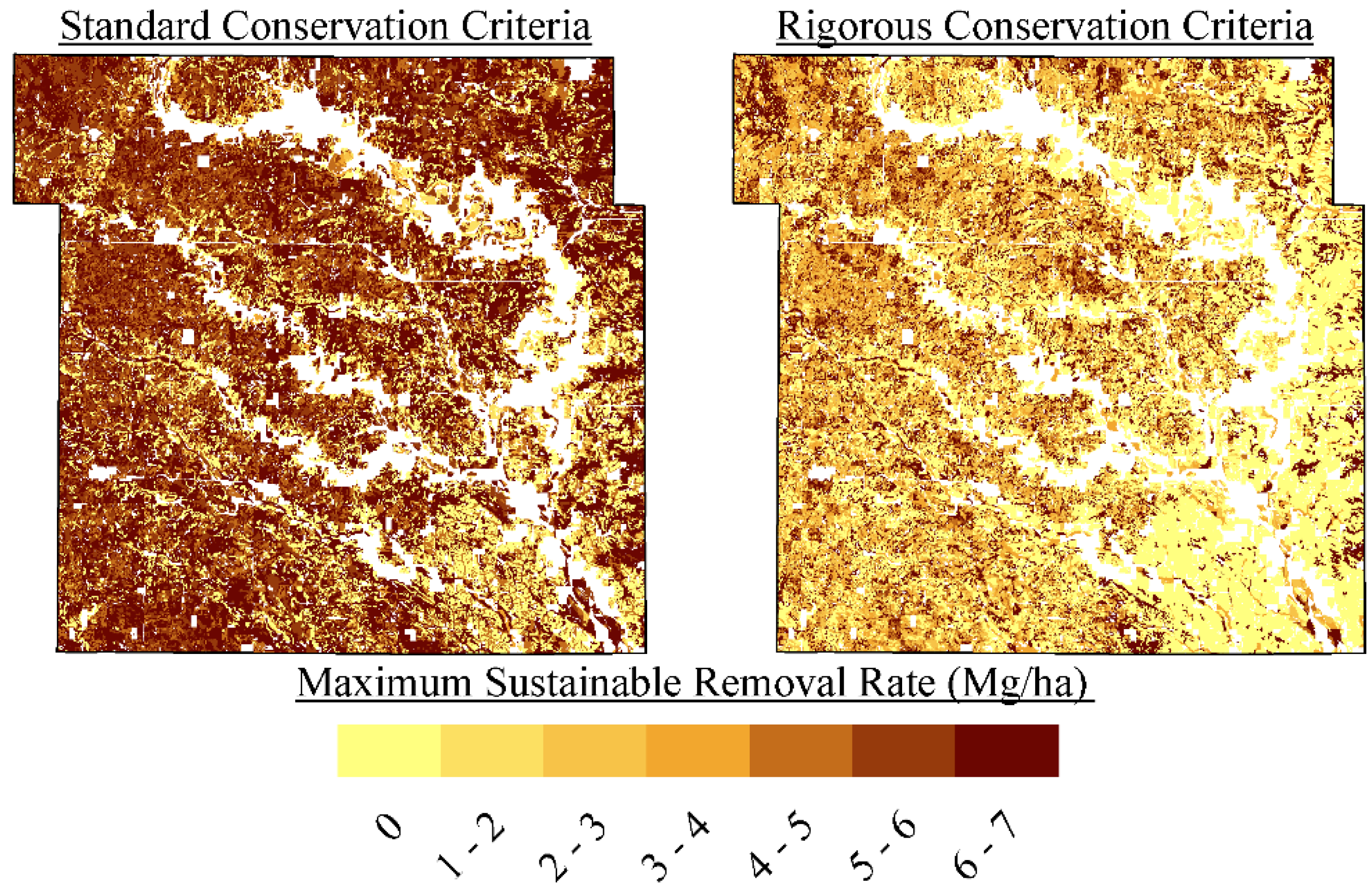
3.1. Production and Sustainably Available Corn Stover

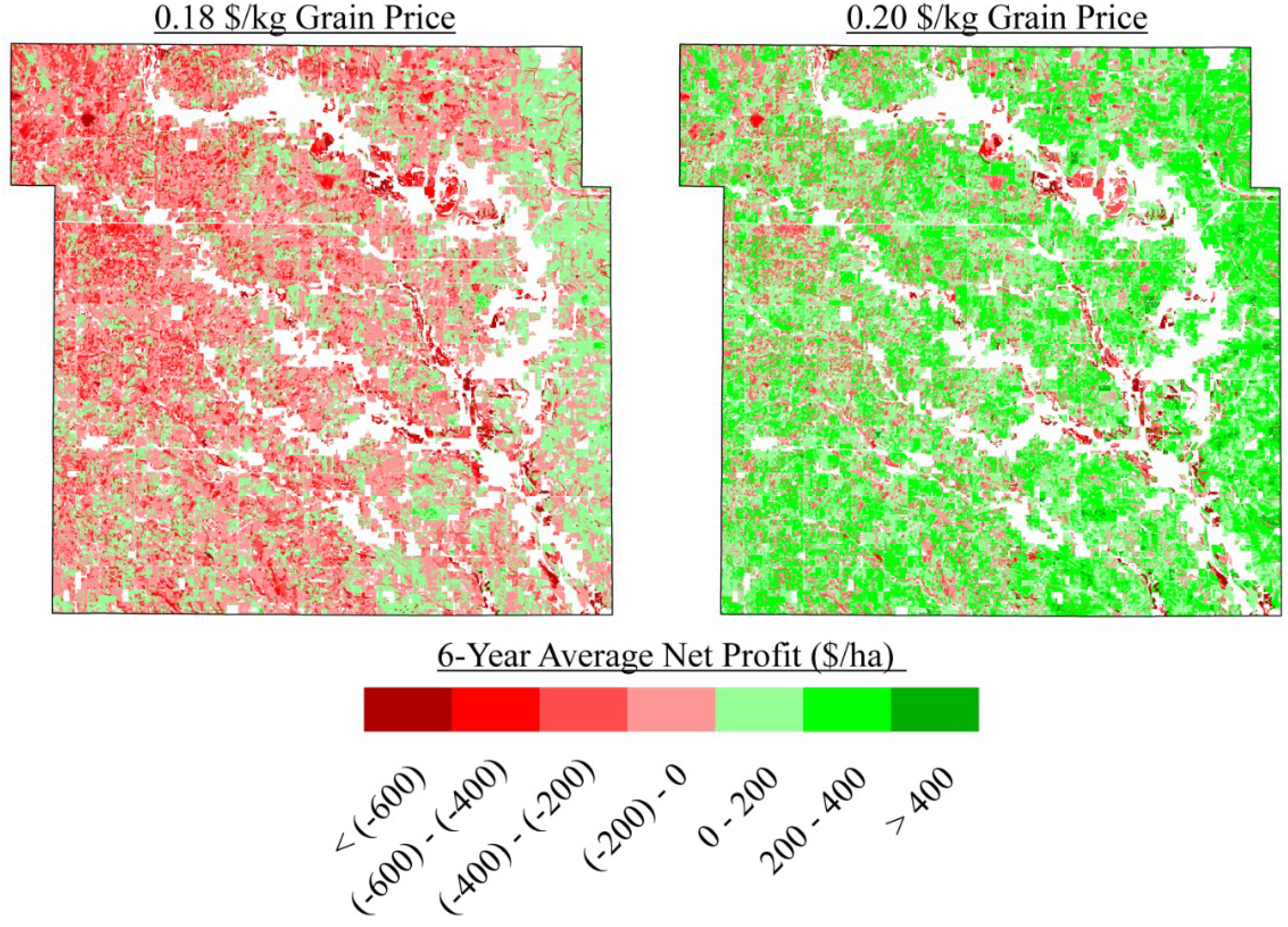
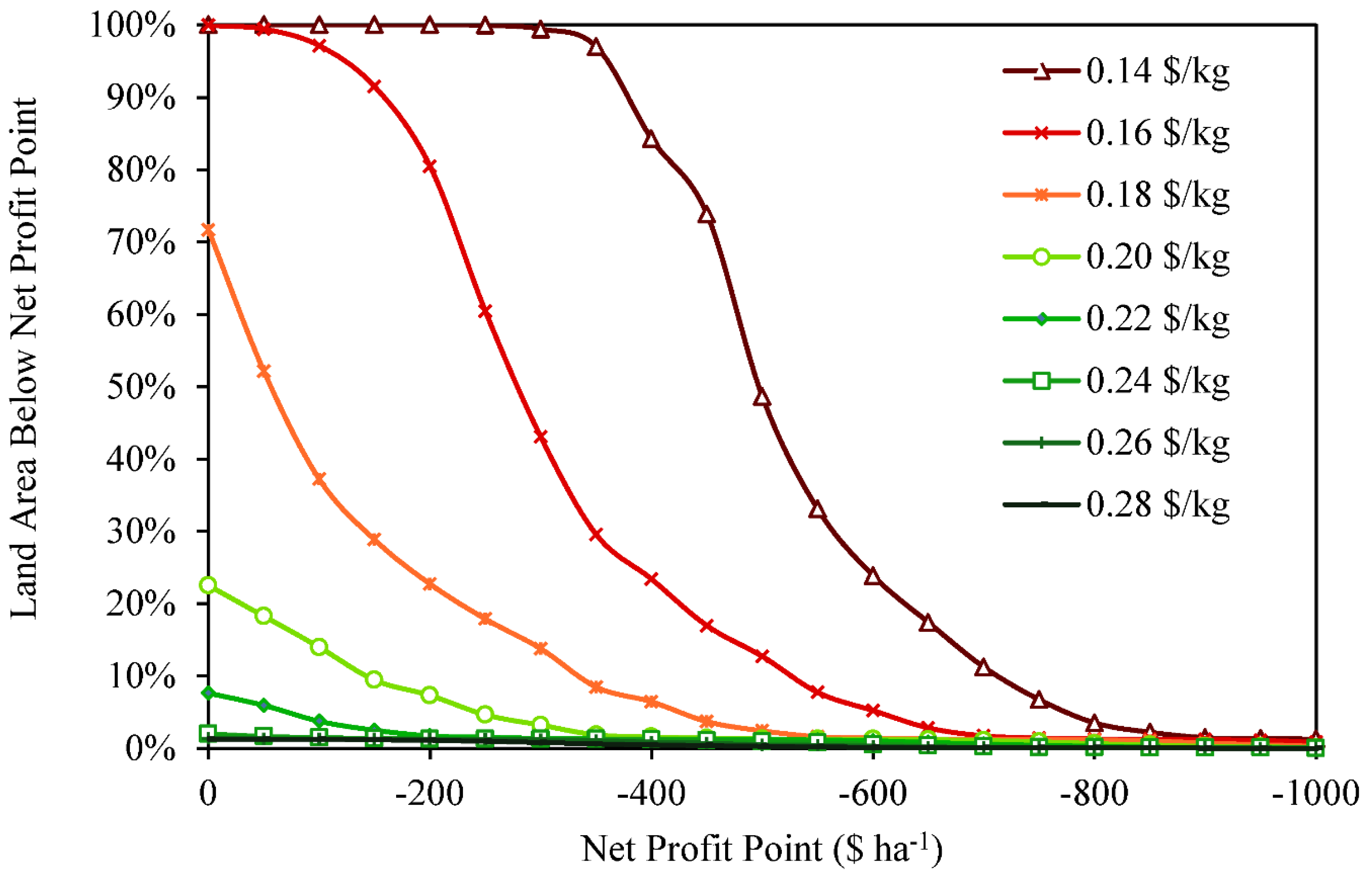
3.2. Profit
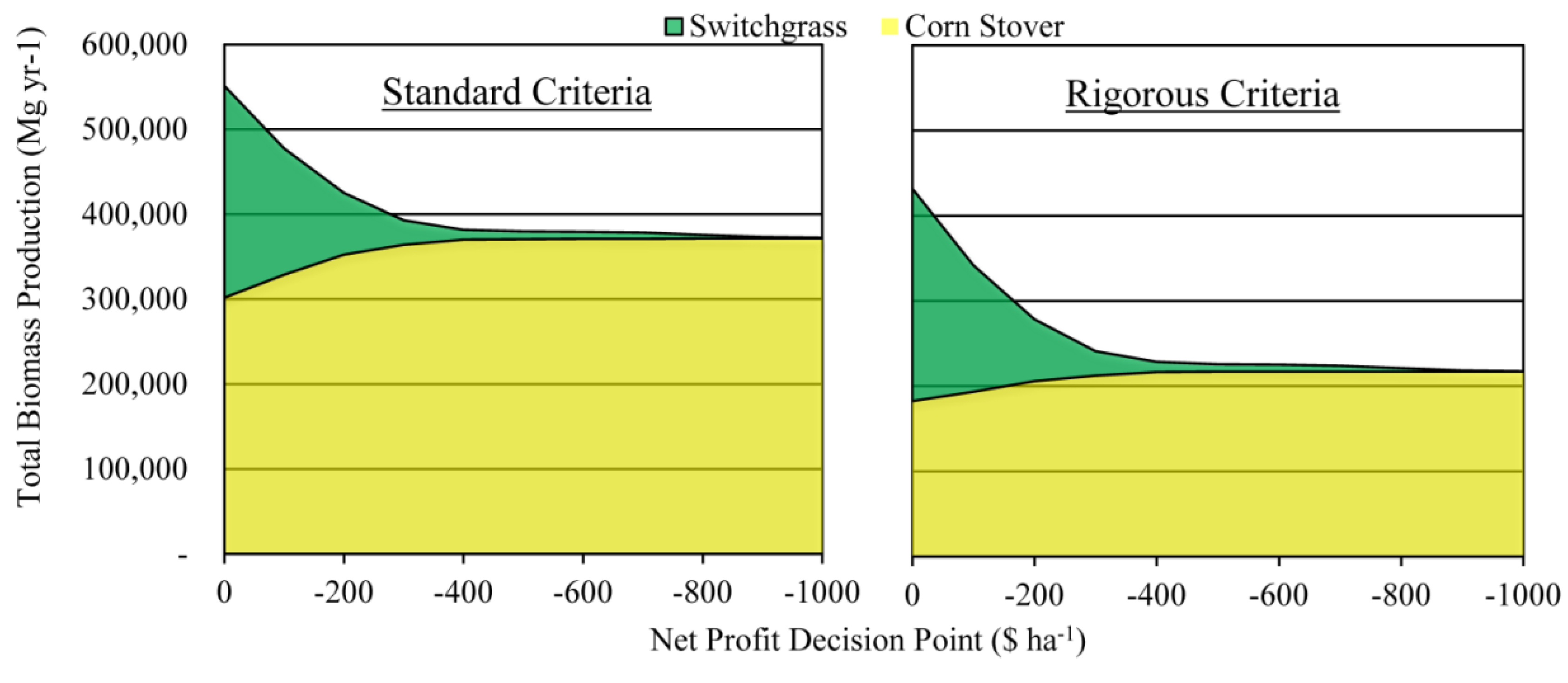
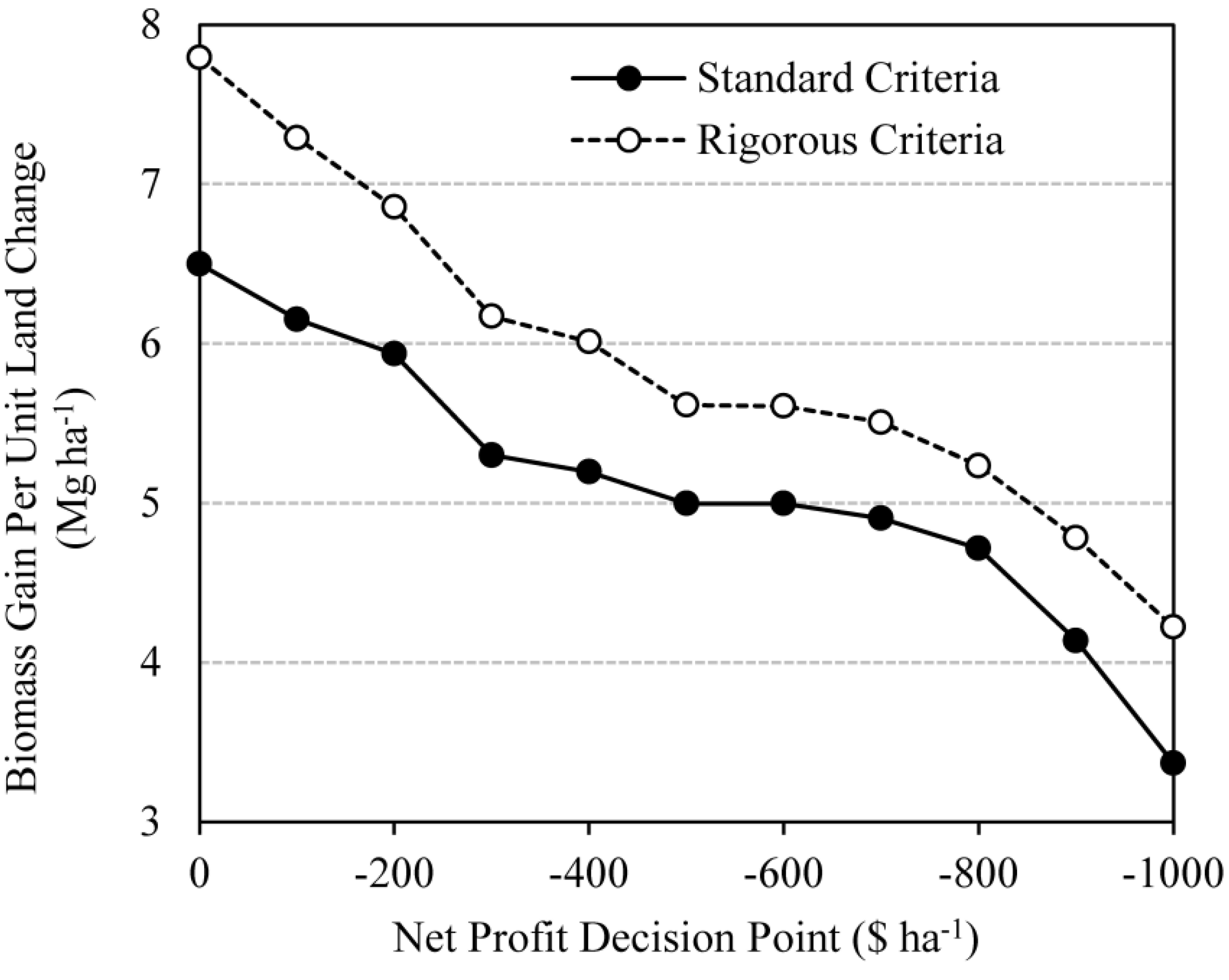
3.3. Opportunity for Energy Crops
3.4. Impact on County-Level Production and Field-Level Profit

| County Level Statistics | Net Profit Decision Point ($·ha−1) | ||||||
|---|---|---|---|---|---|---|---|
| 0 | −100 | −200 | −300 | −400 | −600 | None | |
| Corn Stover Availability, Mg·year−1 | 182,000 | 193,000 | 206,000 | 213,000 | 217,000 | 217,000 | 217,000 |
| Switchgrass Availability, Mg·year−1 | 250,000 | 149,000 | 73,000 | 29,000 | 12,000 | 9,000 | 0 |
| Total Biomass Availability, Mg·year−1 | 432,000 | 342,000 | 278,000 | 241,000 | 228,000 | 226,000 | 217,000 |
| Mass Fraction Corn Stover | 42% | 57% | 74% | 88% | 95% | 96% | 100% |
| Mass Fraction Switchgrass | 58% | 43% | 26% | 12% | 5% | 4% | 0% |
| Annual Biomass Increase a | 99% | 58% | 28% | 11% | 5% | 4% | - |
| Land Conversion | 22% | 14% | 7% | 3% | 2% | 1% | - |
| Fields Affected | 85% | 74% | 57% | 30% | 16% | 15% | - |
| Mean Field Level Area Change b | 25% | 18% | 12% | 10% | 10% | 9% | - |
| Mean Field Level Profit, $·ha−1c | 198 | 174 | 151 | 134 | 127 | 125 | 113 |
| Field Level Profit Std.Dev, $·ha−1 | 92 | 127 | 157 | 175 | 183 | 185 | 205 |
| Profit Variance Between Fields | 49% | 39% | 36% | 37% | 38% | 38% | 41% |
| Profit Variance Within Fields | 51% | 61% | 64% | 63% | 62% | 62% | 59% |
| Reduction in Total Profit Variance | 78% | 65% | 50% | 36% | 28% | 25% | - |

4. Conclusions
Acknowledgments
U.S. Department of Energy Disclaimer
Author Contributions
Conflicts of Interest
References
- Perlack, R.D.; Stokes, B.J. Billion-Ton Update: Biomass Supply for a Bioenergy and Bioproducts Industry; ORNL/TM-2011/224; Oak Ridge National Laboratory: Oak Ridge, TN, USA, 2011. [Google Scholar]
- Hess, J.R.; Wright, C.T.; Kenney, K.L.; Searcy, E.M. Uniform-Format Solid Feedstock Supply System: A Commodity-Scale Design to Produce an Infrastructure-Compatible Bulk Solid from Lignocellulosic Biomass—Executive Summary; Idaho National Laboratory (INL): Idaho Falls, IA, USA, 2009. [Google Scholar]
- Hess, J.R.; Wright, C.T.; Kenney, K.L. Cellulosic biomass feedstocks and logistics for ethanol production. Biofuels Bioprod. Biorefin. 2007, 1, 181–190. [Google Scholar] [CrossRef]
- Graham, R.L.; Nelson, R.; Sheehan, J.; Perlack, R.; Wright, L.L. Current and potential US corn stover supplies. Agron. J. 2007, 99, 1–11. [Google Scholar] [CrossRef]
- Searcy, E.; Hess, J.R.; Tumuluru, J.; Ovard, L.; Muth, D.; Trømborg, E.; Wild, M.; Deutmeyer, M.; Nikolaisen, L.; Ranta, T.; et al. Optimization of Biomass Transport and Logistics. In International Bioenergy Trade; Junginger, M., Goh, C.S., Faaij, A., Eds.; Springer Netherlands: Dordrecht, The Netherlands, 2014; Volume 17, pp. 103–123. [Google Scholar]
- U.S. Congress. Energy Independence and Security Act of 2007. Public Law 110–140. Available online: http://www.govtrack.us/congress/bills/110/hr116 (accessed on 7 October 2014).
- Wilhelm, W.W.; Hess, R.J.; Karlen, D.L.; Johnson, J.M.F.; Muth, D.J.; Baker, J.M.; Gollany, H.T.; Novak, J.M.; Stott, D.E.; Varvel, G.E. Review: Balancing limiting factors & economic drivers for sustainable Midwestern US agricultural residue feedstock supplies. Ind. Biotechnol. 2010, 6, 271–287. [Google Scholar] [CrossRef]
- Muth, D.J.; Bryden, K.M.; Nelson, R.G. Sustainable agricultural residue removal for bioenergy: A spatially comprehensive US national assessment. Appl. Energy 2013, 102, 403–417. [Google Scholar] [CrossRef]
- Bergtold, J.; Fewell, J.; Williams, J. Farmers’ willingness to produce alternative cellulosic biofuel feedstocks under contract in kansas using stated choice experiments. Bioenerg. Res. 2014, 7, 876–884. [Google Scholar] [CrossRef]
- Paine, L.K.; Peterson, T.L.; Undersander, D.J.; Rineer, K.C.; Bartelt, G.A.; Temple, S.A.; Sample, D.W.; Klemme, R.M. Some ecological and socio-economic considerations for biomass energy crop production. Biomass Bioenergy 1996, 10, 231–242. [Google Scholar] [CrossRef]
- Walsh, M.E.; Daniel, G.; Shapouri, H.; Slinsky, S.P. Bioenergy crop production in the United States: Potential quantities, land use changes, and economic impacts on the agricultural sector. Environ. Res. Econ. 2003, 24, 313–333. [Google Scholar] [CrossRef]
- Johnson, J.M.F.; Coleman, M.D.; Gesch, R.; Jaradat, A.; Mitchell, R.; Reicosky, D.; Wilhelm, W.W. Biomass-bioenergy crops in the United States: A changing paradigm. Am. J. Plant Sci. Biotechnol. 2007, 1, 1–28. [Google Scholar]
- Wullschleger, S.D.; Davis, E.B.; Borsuk, M.E.; Gunderson, C.A.; Lynd, L.R. Biomass production in switchgrass across the United States: Database description and determinants of yield. Agron. J. 2010, 102, 1158–1168. [Google Scholar] [CrossRef]
- Guretzky, J.; Biermacher, J.; Cook, B.; Kering, M.; Mosali, J. Switchgrass for forage and bioenergy: Harvest and nitrogen rate effects on biomass yields and nutrient composition. Plant Soil 2011, 339, 69–81. [Google Scholar] [CrossRef]
- Arundale, R.; Dohleman, F.; Voigt, T.; Long, S. Nitrogen fertilization does significantly increase yields of stands of Miscanthus × giganteus and Panicum virgatum in multiyear trials in Illinois. Bioenerg. Res. 2014, 7, 408–416. [Google Scholar] [CrossRef]
- Heaton, E.A.; Dohleman, F.G.; Long, S.P. Meeting US biofuel goals with less land: The potential of Miscanthus. Glob. Chang. Biol. 2008, 14, 2000–2014. [Google Scholar] [CrossRef]
- Schmer, M.R.; Liebig, M.; Vogel, K.; Mitchell, R.B. Field-scale soil property changes under switchgrass managed for bioenergy. GCB Bioenergy 2011, 3, 439–448. [Google Scholar] [CrossRef]
- Follett, R.; Vogel, K.; Varvel, G.; Mitchell, R.; Kimble, J. Soil carbon sequestration by switchgrass and no-till maize grown for bioenergy. Bioenergy Res. 2012, 5, 866–875. [Google Scholar] [CrossRef]
- Blanco-Canqui, H.; Gantzer, C.J.; Anderson, S.H.; Alberts, E.E.; Thompson, A.L. Grass barrier and vegetative filter strip effectiveness in reducing runoff, sediment, nitrogen, and phosphorus loss. Soil Sci. Soc. Am. J. 2004, 68, 1670–1678. [Google Scholar] [CrossRef]
- Werling, B.P.; Dickson, T.L.; Isaacs, R.; Gaines, H.; Gratton, C.; Gross, K.L.; Liere, H.; Malmstrom, C.M.; Meehan, T.D.; Ruan, L.; et al. Perennial grasslands enhance biodiversity and multiple ecosystem services in bioenergy landscapes. Proc. Natl. Acad. Sci. USA 2014, 111, 1652–1657. [Google Scholar] [CrossRef] [PubMed]
- Hartman, J.C.; Nippert, J.B.; Orozco, R.A.; Springer, C.J. Potential ecological impacts of switchgrass (Panicum virgatum L.) biofuel cultivation in the Central Great Plains, USA. Biomass Bioenergy 2011, 35, 3415–3421. [Google Scholar] [CrossRef]
- Atwell, R.C.; Schulte, L.A.; Westphal, L.M. How to build multifunctional agricultural landscapes in the U.S. Corn Belt: Add perennials and partnerships. Land Use Policy 2010, 27, 1082–1090. [Google Scholar] [CrossRef]
- Larson, J.; English, B.; Hellwinckel, C.; Ugarte, D.D.L.T.; Walsh, M. A farm-level evaluation of conditions under which farmers will supply biomass feedstocks for energy production. In Proceedings of the 2005 American Agricultural Economics Association Annual Meeting, Providence, RI, USA, 24–27 July 2005; pp. 24–27.
- Soule, M.J.; Tegene, A.; Wiebe, K.D. Land tenure and the adoption of conservation practices. Am. J. Agric. Econ. 2000, 82, 993–1005. [Google Scholar] [CrossRef]
- Hendricks, N.P.; Sinnathamby, S.; Douglas-Mankin, K.; Smith, A.; Sumner, D.A.; Earnhart, D.H. The Environmental Effects of Crop Price Increases: Nitrogen Losses in the US Corn Belt. Available online: https://files.are.ucdavis.edu/uploads/filer_public/2014/06/19/water_quality_5-22-14.pdf (accessed on 7 October 2014).
- Smith, D.J.; Schulman, C.; Current, D.; Easter, K.W. Willingness of agricultural landowners to supply perennial energy crops. In Proceedings of the Agricultural and Applied Economics Association & NAREA Joint Annual Meeting, Pittsburgh, PA, USA, 24–26 July 2011.
- James, L.K.; Swinton, S.M.; Thelen, K.D. Profitability analysis of cellulosic energy crops compared with corn. Agron. J. 2010, 102, 675–687. [Google Scholar] [CrossRef]
- Kyveryga, P.M.; Blackmer, T.M.; Caragea, P.C. Categorical analysis of spatial variability in economic yield response of corn to nitrogen fertilization. Agron. J. 2011, 103, 796–804. [Google Scholar] [CrossRef]
- Daughtry, C.S.T.; Doraiswamy, P.C.; Hunt, E.R., Jr.; Stern, A.J.; McMurtrey Iii, J.E.; Prueger, J.H. Remote sensing of crop residue cover and soil tillage intensity. Soil Tillage Res. 2006, 91, 101–108. [Google Scholar] [CrossRef]
- Tomer, M.D.; Porter, S.A.; James, D.E.; Boomer, K.M.B.; Kostel, J.A.; McLellan, E. Combining precision conservation technologies into a flexible framework to facilitate agricultural watershed planning. J. Soil Water Conserv. 2013, 68, 113A–120A. [Google Scholar] [CrossRef]
- Muth, D.J.; McCorkle, D.S.; Koch, J.B.; Bryden, K.M. Modeling sustainable agricultural residue removal at the subfield scale. Agron. J. 2012, 104, 970–981. [Google Scholar] [CrossRef]
- Abodeely, J.M.; Muth, D.J.; Koch, J.B.; Bryden, K.M. A model integration framework for assessing integrated landscape management strategies. In Environmental Software Systems. Fostering Information Sharing; Hřebíček, J., Schimak, G., Kubásek, M., Rizzoli, A., Eds.; Springer: Berlin, Germany, 2013; Volume 413, pp. 121–128. [Google Scholar]
- Soil Survey Staff. Web Soil Survey. US Department of Agriculture Natural Resources Conservation Service: Washington, DC, USA. Available online: http://websoilsurvey.nrcs.usda.gov/ (accessed on 6 March 2014).
- Muth, D.J.; Bryden, K.M. An integrated model for assessment of sustainable agricultural residue removal limits for bioenergy systems. Environ. Model. Softw. 2013, 39, 50–69. [Google Scholar]
- USDA National Agricultural Statistics Service Data and Statistics, 2014. In Quick Stats Online Database Tool. Available online: http://www.nass.usda.gov/Data_and_Statistics/ (accessed on 6 March 2014).
- Farm Service Agency. 2012; Imagery Programs: NAIP imagery. US Department of Agriculture Farm Service Agency: Washington, DC, USA. Available online: http://www.fsa.usda.gov/FSA/apfoapp?area=home&subject=prog&topic=nai (accessed on 7 October 2014). [Google Scholar]
- USDA National Agricultural Statistics Service Cropland Data Layer, 2014. Published Crop-Specific Data Layer. Available online: http://nassgeodata.gmu.edu/CropScape/ (accessed on 6 March 2014).
- Miller, G.A.; Fenton, T.E.; Oneal, B.R.; Tiffany, B.J.; Burras, C.E. Iowa Soil Properties and Interpretations Database, ISPAID Version 7.3. Iowa State University Extension. 2010. Available online: http://www.extension.iastate.edu/soils/ispaid (accessed on 7 October 2014).
- Wilson, D.M.; Heaton, E.A.; Schulte, L.A.; Gunther, T.P.; Shea, M.E.; Hall, R.B.; Headlee, W.L.; Moore, K.J.; Boersma, N.N. Establishment and short-term productivity of annual and perennial bioenergy crops across a landscape gradient. Bioenerg. Res. 2014, 7, 885–898. [Google Scholar] [CrossRef]
- Heggenstaller, A.H.; Moore, K.J.; Liebman, M.; Anex, R.P. Nitrogen influences biomass and nutrient partitioning by perennial, warm-season grasses. Agron. J. 2009, 101, 1363–1371. [Google Scholar] [CrossRef]
- McLaughlin, S.B.; Adams Kszos, L. Development of switchgrass (Panicum virgatum) as a bioenergy feedstock in the United States. Biomass Bioenergy 2005, 28, 515–535. [Google Scholar] [CrossRef]
- Estimated Costs of Crop Production in Iowa—2014. Iowa State University Extension and Outreach. Available online: http://www.extension.iastate.edu/agdm/crops/html/a1-20.html (accessed on 7 October 2014).
- Cash Rental Rates for Iowa 2014 Survey. File C2–10. Iowa State University Extension and Outreach. Available online: http://www.extension.iastate.edu/agdm/wholefarm/pdf/c2-10.pdf (accessed on 6 March 2014).
- Revised Universal Soil Loss Equation, Version 2 (RUSLE2). Official NRCS RUSLE2 Program; USDA Natural Resource Conservation Service and USDA Agricultural Research Service: Washington, DC, USA. Available online: http://fargo.nserl.purdue.edu/rusle2_dataweb/RUSLE2_Index.htm (accessed on 7 October 2014).
- Official NRCS-WEPS Site. Wind Erosion Prediction System. USDA Agricultural Research Service and USDA Natural Resource Conservation Service: Washington, DC, USA. Available online: http://www.weru.ksu.edu/nrcs/wepsnrcs.html (accessed on 7 October 2014).
- Soil Conditioning Index. US Department of Agriculture Natural Resource Conservation Service: Washington, DC, USA. Available online: http://www.nrcs.usda.gov/wps/portal/nrcs/detail/ia/newsroom/factsheets/?cid=nrcs142p2_008548 (accessed on 7 October 2014).
- Bonner, I.J.; Muth, D.J., Jr.; Koch, J.B.; Karlen, D.L. Modeled impacts of cover crops and vegetative barriers on corn stover availability and soil quality. Bioenerg. Res. 2014, 7, 576–589. [Google Scholar] [CrossRef]
- Conservation Technology Information Center. Purdue University: West Lafayette, IN, USA. Available online: http://www.ctic.purdue.edu/ (accessed on 7 October 2014).
- Crop Management Zones. US Department of Agriculture Natural Resource Conservation Service: Washington, DC, USA. Available online: http://fargo.nserl.purdue.edu/rusle2_dataweb/NRCS_Crop_Management_Zone_Maps.htm (accessed on 7 October 2014).
- Iowa NRCS Soils Program. US Department of Agriculture: Washington, DC, USA. Available online: http://www.nrcs.usda.gov/wps/portal/nrcs/main/ia/soils/ (accessed 6 March 2014).
© 2014 by the authors; licensee MDPI, Basel, Switzerland. This article is an open access article distributed under the terms and conditions of the Creative Commons Attribution license (http://creativecommons.org/licenses/by/4.0/).
Share and Cite
Bonner, I.J.; Cafferty, K.G.; Muth, D.J., Jr.; Tomer, M.D.; James, D.E.; Porter, S.A.; Karlen, D.L. Opportunities for Energy Crop Production Based on Subfield Scale Distribution of Profitability. Energies 2014, 7, 6509-6526. https://doi.org/10.3390/en7106509
Bonner IJ, Cafferty KG, Muth DJ Jr., Tomer MD, James DE, Porter SA, Karlen DL. Opportunities for Energy Crop Production Based on Subfield Scale Distribution of Profitability. Energies. 2014; 7(10):6509-6526. https://doi.org/10.3390/en7106509
Chicago/Turabian StyleBonner, Ian J., Kara G. Cafferty, David J. Muth, Jr., Mark D. Tomer, David E. James, Sarah A. Porter, and Douglas L. Karlen. 2014. "Opportunities for Energy Crop Production Based on Subfield Scale Distribution of Profitability" Energies 7, no. 10: 6509-6526. https://doi.org/10.3390/en7106509
APA StyleBonner, I. J., Cafferty, K. G., Muth, D. J., Jr., Tomer, M. D., James, D. E., Porter, S. A., & Karlen, D. L. (2014). Opportunities for Energy Crop Production Based on Subfield Scale Distribution of Profitability. Energies, 7(10), 6509-6526. https://doi.org/10.3390/en7106509