A Co-Powered Biomass and Concentrated Solar Power Rankine Cycle Concept for Small Size Combined Heat and Power Generation


Abstract
:1. Introduction
2. Co-Powered Solar-Biomass Plant and Model Description
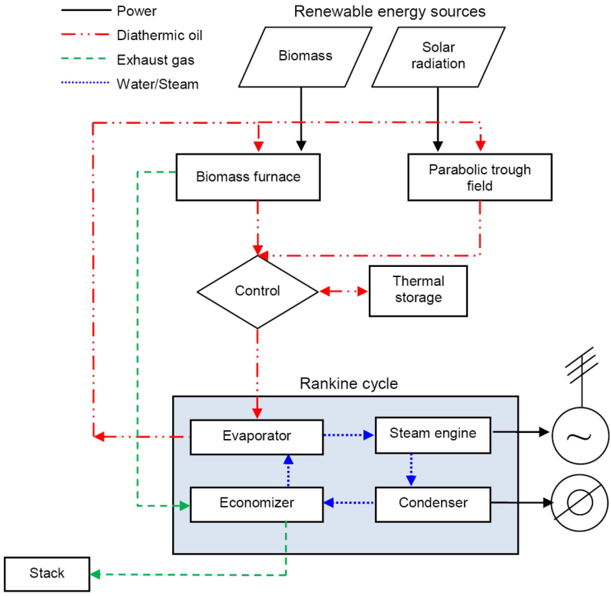
2.1. Component and System Description


| Component description | Size | |
|---|---|---|
| Solar parabolic trough field (2,580 m2) | kWth | 1,200 |
| TES | GJ | 57 |
| Biomass furnace | kWth | 1,163 |
| Reciprocating steam engine | kWel | 130 |
| Condenser | kWth | 1,240 |
| Diathermic oil circuit | ||
| Maximum/minimum temperature | °C | 300/240 |
| Maximum/minimum specific heat | kJ/kg K | 2.36/2.19 |
| Operating pressure | kPa | 800 |
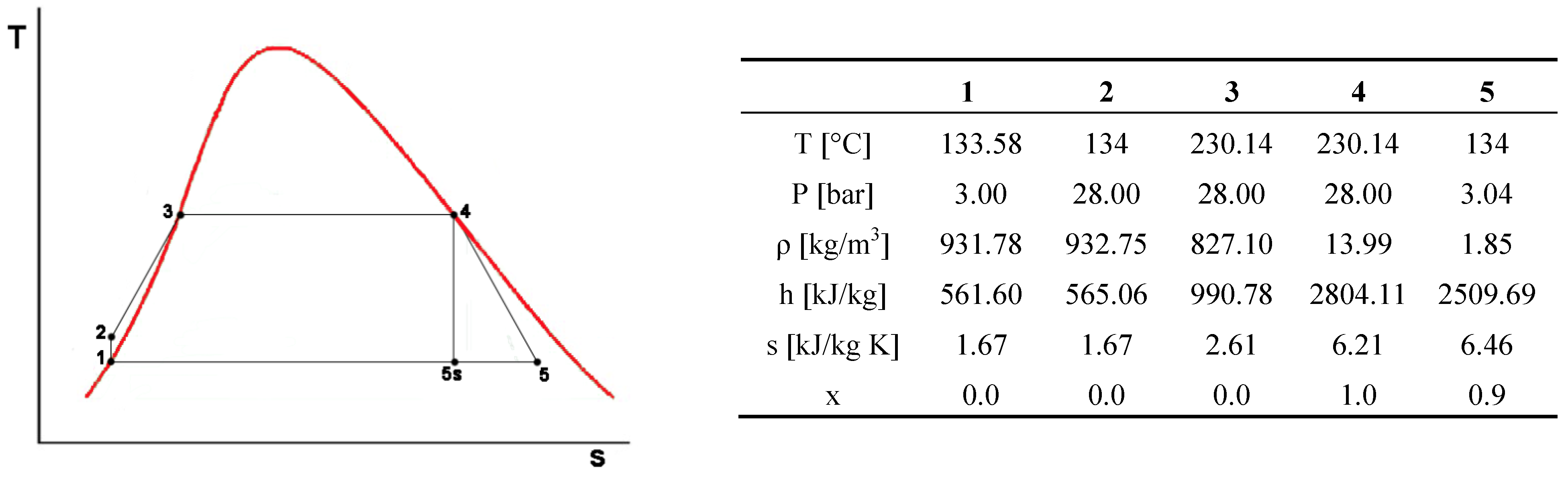
| Water/Steam circuit | ||
| Maximum/minimum pressure | kPa | 2,800/300 |
| Maximum/minimum temperature | °C | 230/134 |
| Water/steam mass flow rate | kg/s | 0.51 |
| Electric power | kW | 130 |
| Thermal power | kW | 1,100 |

2.2. Transient Model Description
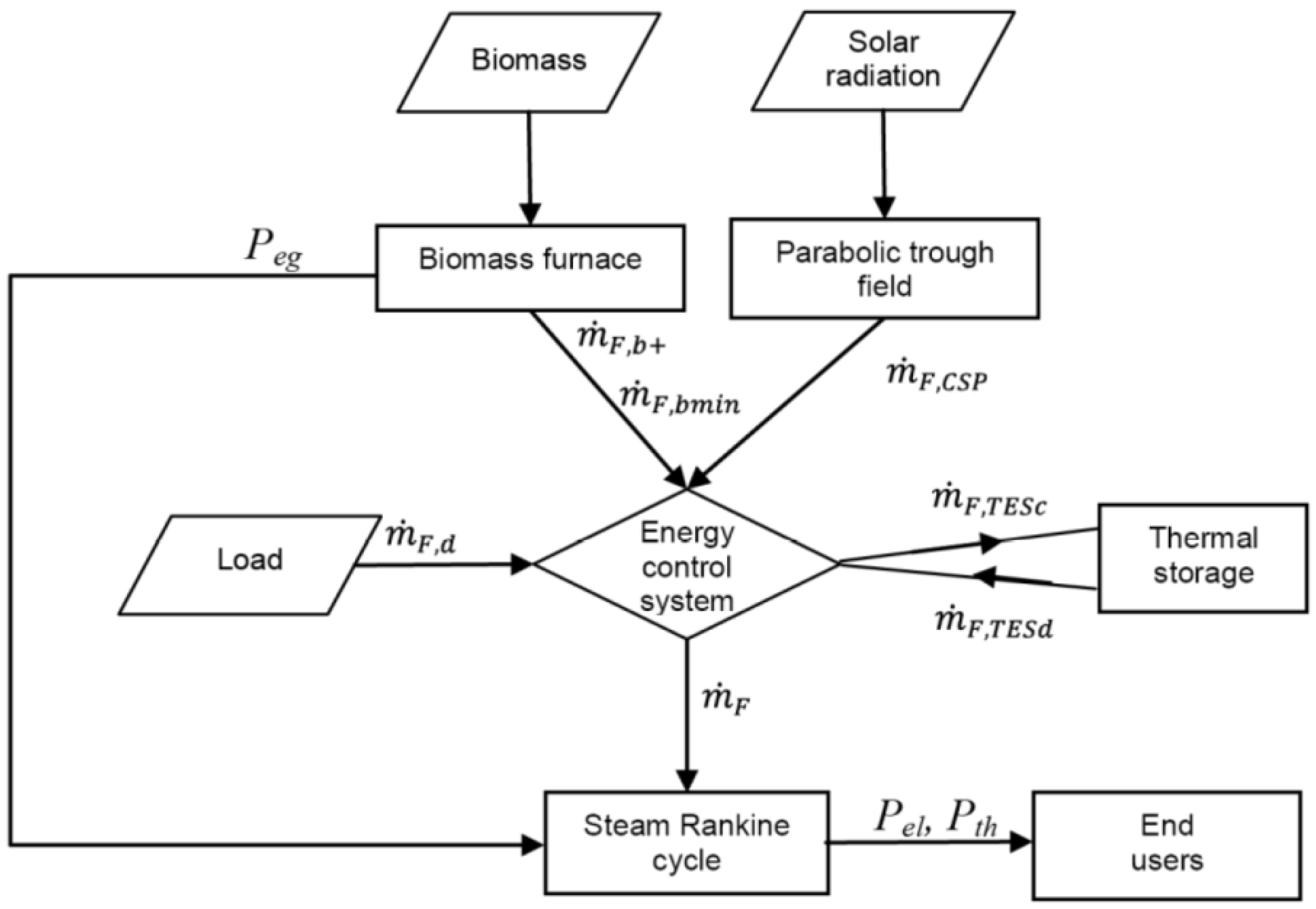
- direct CSP contribution surplus, the exceeding HTF flow rate will first be sent to the TES (flow rate ) and then dumped;
- direct CSP contribution deficit, the missing heat flux will be first requested to the TES (flow rate ); and
- in case of insufficient flux from the solar section (flow rate ) and minimum biomass contributions, an additional heat flux is requested to the biomass furnace (flow rate ).
3. End User Description
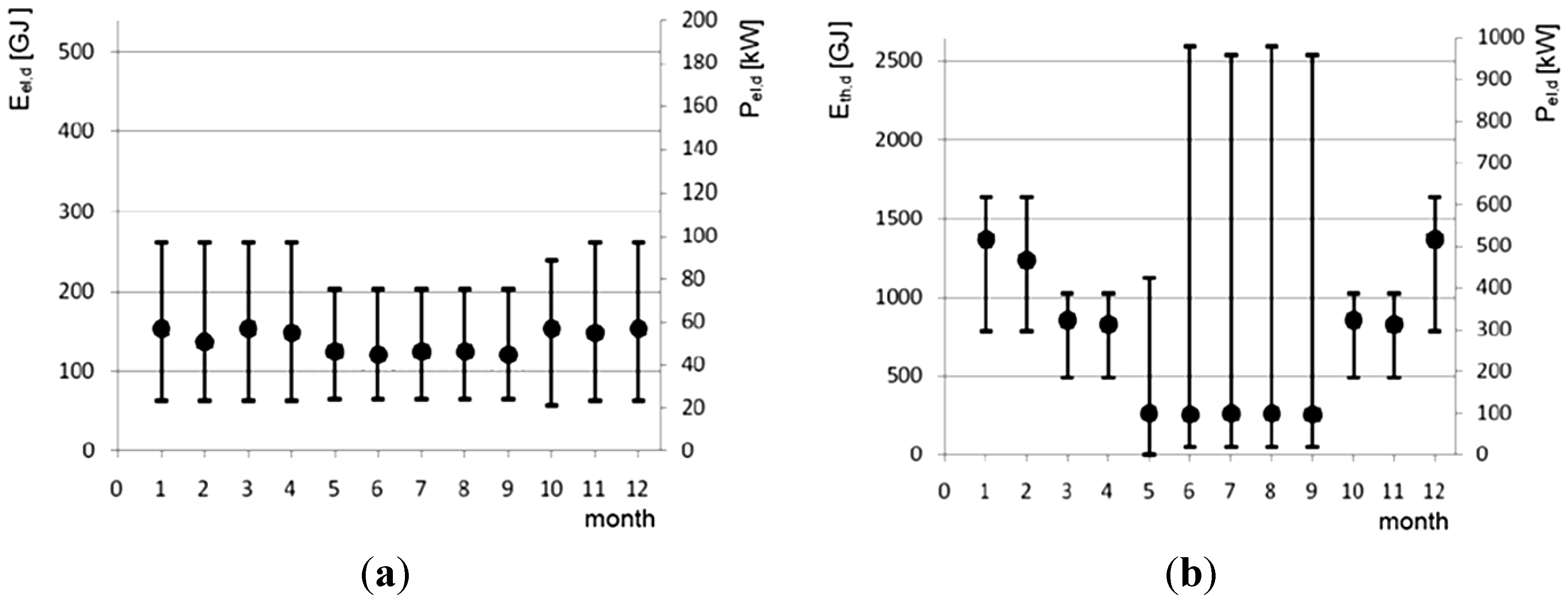
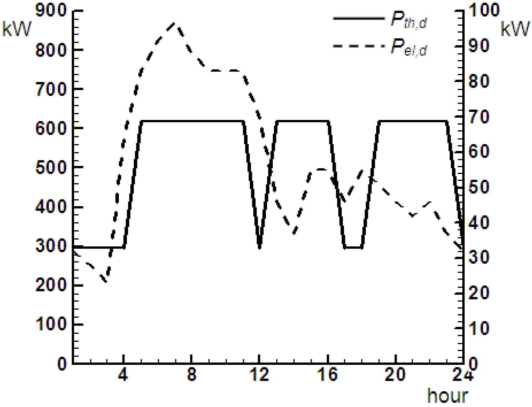
3.1. End-User Load Profile
| Type/Category | Business/leisure, 4 stars |
| Location | Industrial site |
| Activities | restaurants, bars, conference rooms, laundry |
| Number of rooms | 190 |
| Number of sleeping accommodations | 350 |
| Volume [m3] | 43,000 |
| Area [m2] | 8,900 |
| Heat load [GJ/y] | 8,640 |
| Electric load [GJ/y] | 1,656 |
| Cooling load [GJ/y] | 2,580 |
| Equivalent thermal load [GJ/y] | 12,326 |
| Heat/electric consumption ratio [GJth/GJel] | 5.23 |
| Equivalent heat/electric consumption ratio [GJth/GJel] | 7.44 |
3.2. RES Data Input
| Hour | DNI [W/m2] | Dry bulb temperature [°C] | Hour | DNI [W/m2] | Dry bulb temperature [°C] |
|---|---|---|---|---|---|
| 1 | 0 | 8.20 | 13 | 902.50 | 11.70 |
| 2 | 0 | 8.30 | 14 | 902.50 | 12.70 |
| 3 | 0 | 7.95 | 15 | 879.72 | 14.10 |
| 4 | 0 | 7.75 | 16 | 806.39 | 15.20 |
| 5 | 0 | 7.20 | 17 | 587.22 | 15.10 |
| 6 | 0 | 6.30 | 18 | 82.50 | 14.45 |
| 7 | 0 | 5.95 | 19 | 0.28 | 13.55 |
| 8 | 0.28 | 7.05 | 20 | 0 | 12.20 |
| 9 | 82.50 | 8.40 | 21 | 0 | 11.05 |
| 10 | 587.22 | 8.55 | 22 | 0 | 10.65 |
| 11 | 806.39 | 8.90 | 23 | 0 | 11.10 |
| 12 | 879.72 | 10.25 | 24 | 0 | 10.95 |
4. Solar-Biomass Power Plant Performance
4.1. Overall Performance
| Electric Tracking | Thermal Tracking | ||
|---|---|---|---|
| RES system | Solar energy [GJ/y] | 4,277.53 | 4,277.53 |
| Effective solar energy supply [GJ/y] | 4,172.09 | 4,092.72 | |
| Biomass energy [GJ/y] | 18,132.39 | 17,221.31 | |
| Solar fraction | 18.71 | 19.20 | |
| Biomass consumption [ton/y] | 990.84 | 941.06 | |
| Global effective energy input Eg [GJ/y] | 22,304.48 | 21,314.03 | |
| Electric output | Plant electric energy output Eel [GJ/y] | 2,064.37 | 2,017.10 |
| Eel,d [GJ/y] | 1,664.68 | 1,664.46 | |
| Eel/Eel,d [%] | 124.01 | 121.19 | |
| Surplus [%] | 19.80 | 25.80 | |
| Deficit [%] | −0.44 | −8.32 | |
| Thermal output | Plant thermal energy supply Eth [GJ/y] | 17,291.93 | 16,895.49 |
| Eth,d [GJ/y] | 11,656.13 | 11,653.99 | |
| Eth/Eth,d [%] | 148.35 | 144.98 | |
| Surplus [%] | 40.09 | 33.27 | |
| Deficit [%] | −7.49 | −2.26 | |
| RC system | Net electric efficiency = Eel/Eg [%] | 9.26 | 9.46 |
| Net thermal efficiency = Eth/Eg [%] | 77.53 | 79.27 | |
| Electric index = Eel/Eth [%] | 11.94 | 11.94 | |
| Primary energy ratio = (Eel/ηel + Eth/ηth)/Eg [-] † | 1.21 | 1.24 |
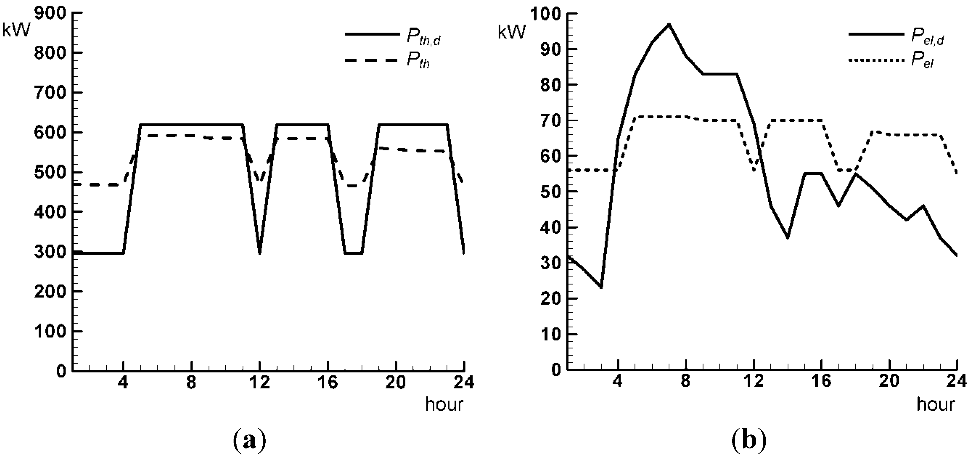
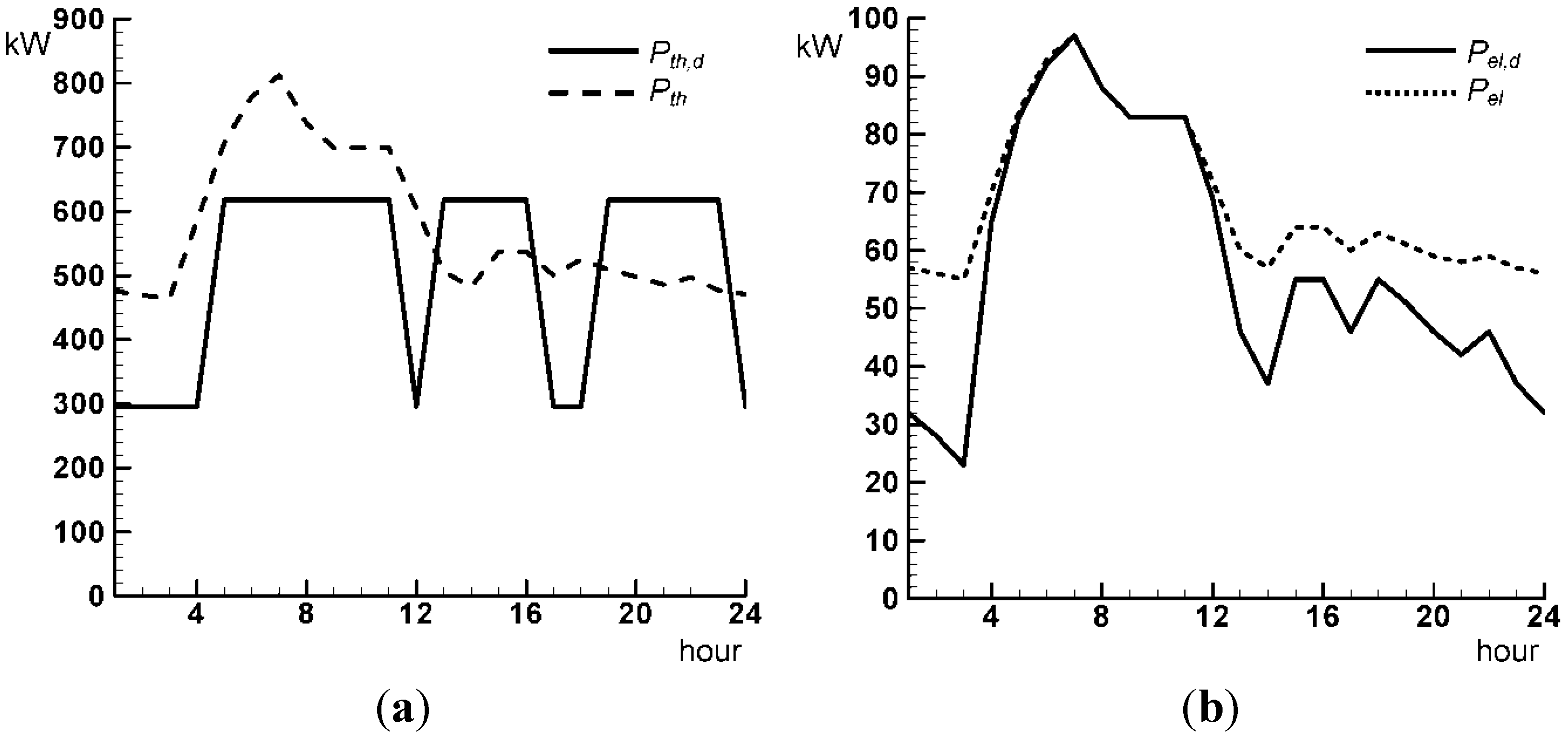
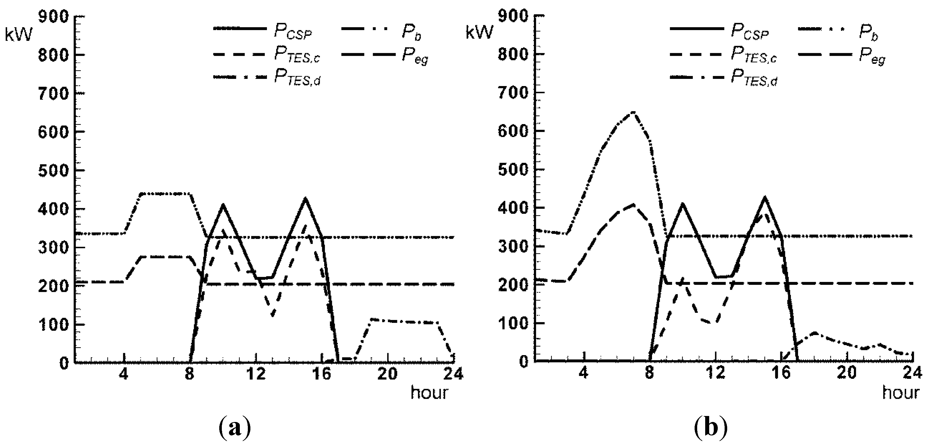
4.2. Hourly Power System Performance
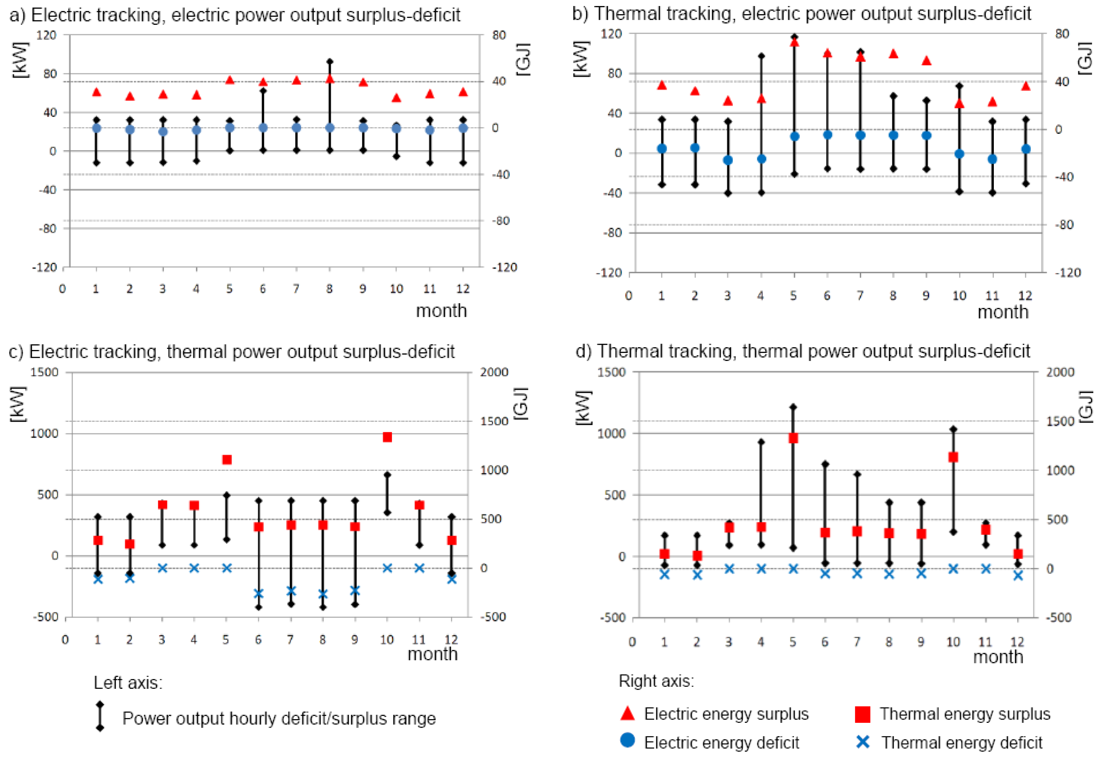
4.3. Matching Through the Load Tracking


5. Environmental Issues
| Electric tracking | Thermal tracking | |
|---|---|---|
| CO2 [ton/y] | 2,967.87 | 3,442.71 |
| SOx [ton/y] | 3.09 | 3.59 |
| NOx [ton/y] | 1.85 | 2.15 |
| TSP [ton/y] | 0.12 | 0.14 |
| Net land use | |
|---|---|
| Solar field | 6,780 m2 |
| TES | 570 m2 |
| Biomass furnace, filter and stack | 700 m2 |
| Biomass storage | 3,000 |
| Buildings (Rankine cycle elements, desalting units, offices) | 2,100 |
| Total | 13,150 m2 |
| Technology | Cost [€] |
|---|---|
| CSP field with TES | 7,870,000 |
| Biomass furnace | 130,000 |
| Economizer | 15,000 |
| Evaporator | 45,000 |
| Steam engine | 220,000 |
| Condenser | 15,000 |
| Utilities | 300,000 |
| Total | 8,595,000 |
6. Conclusions
Nomenclature
| Eel | Electric energy output (GJ) |
| Eel,d | Electric energy demand (GJ) |
| Eg | Global energy input from biomass and solar radiation (GJ) |
| Eth | Thermal energy output (GJ) |
| Eth,d | Thermal energy demand (GJ) |
| h | Enthalpy (kJ/kg) |
HTF flow rate (m3/h) | |
Solar field HTF delivered flow rate (m3/h) | |
Minimum biomass furnace HTF delivered flow rate (m3/h) | |
Additional biomass furnace HTF delivered flow rate (m3/h) | |
HTF demanded flow rate (m3/h) | |
Solar direct and TES delivered flow rate (m3/h) | |
TES HTF charge flow rate (m3/h) | |
TES HTF discharge flow rate (m3/h) | |
| P | Pressure (bar) |
| Pb | Biomass derived power (kW) |
| Pb,min | Biomass furnace power at minimum duty (kW) |
| PCSP | CSP derived thermal power (kW) |
| Peg | Exhaust gas power (kW) |
| Pel | Electric power output (kW) |
| Pel,d | Electric load power (kW) |
| PTES,c | Storage charge power (kW) |
| PTES,d | Storage discharge power (kW) |
| Pth | Thermal power output (kW) |
| Pth,d | Thermal load power (kW) |
| s | Entropy (kJ/kg °C) |
| T | Temperature (°C) |
| x |
Vapour fraction (-) |
| δ | Density (kg/m3) |
| ηel | Reference electric efficiency (-) |
| ηth | Reference thermal efficiency (-) |
References
- Maidment, G.G.; Zhao, X.; Riffat, S.B.; Prosser, G. Application of combined heat-and-power and absorption cooling in supermarkets. Appl. Energy 1999, 63, 169–190. [Google Scholar] [CrossRef]
- Maidment, G.G.; Tozer, R.M. Combined cooling heat and power in supermarkets. Appl. Therm. Eng. 2002, 2, 653–665. [Google Scholar] [CrossRef]
- Brown, E.; Mann, M. Initial Market Assessment for Small-Scale Biomass-Based CHP; White Paper, NREL/TP-640-42046; National Renewable Energy Laboratory: Golden, CO, USA, January 2008. [Google Scholar]
- Eastop, T.D.; Croft, D.R. Energy Efficiency for Engineers and Technologists, 1st ed.; Longman Scientific and Technical: Harlow, UK, 1990; p. 335. [Google Scholar]
- Fröhlke, K.; Haidn, O.J. Spinning reserve system based on H2/O2 combustion. Energy Convers. Manage. 1997, 38, 983–993. [Google Scholar] [CrossRef]
- Kélouwani, S.; Agbossou, K.; Chahine, R. Model for energy conversion in renewable energy system with hydrogen storage. J. Power Sources 2005, 140, 392–399. [Google Scholar] [CrossRef]
- Corsini, A.; Rispoli, F.; Gamberale, M.; Tortora, E. Assessment of H2- and H2O-based renewable energy-buffering systems in minor islands. Renew. Energy 2009, 34, 279–288. [Google Scholar] [CrossRef]
- Sinden, G. The Practicalities of Developing Renewable Energy Stand-by Capacity and Intermittency. Submission to the Science and Technology Select Committee of the House of Lords; Environmental Change Institute University of Oxford: Oxford, UK, 2004. [Google Scholar]
- Assessment of Parabolic Trough and Power Tower Solar Technology Cost and Performance Forecasts; NREL Subcontract Report 550-34440; Sargent & Lundy LLC Consulting Group: Chicago, IL, USA, October 2003.
- Solar Process Heat for Production and Advanced Applications; Work Plan, IEA Solar Heating & Cooling Programme Task 49, Solar Paces Programme Task IV; International Energy Agency: Paris, France, October 2011.
- Li, J. Scaling up concentrating solar thermal technology in China. Renew. Sustain. Energy Rev. 2009, 13, 2051–2060. [Google Scholar] [CrossRef]
- Al-Soud, M.S.; Hyayshat, E.S. A 50 MW concentrating solar power plant for Jordan. J. Clean. Prod. 2008, 17, 625–635. [Google Scholar] [CrossRef]
- Dong, L.; Liu, H.; Riffat, S. Development of small-scale and micro-scale biomass fuelled CHP systems. A literature review. Appl. Therm. Eng. 2009, 29, 2119–2126. [Google Scholar] [CrossRef]
- Badami, M.; Mura, M. Preliminary design and controlling strategy of small-scale wood waste Rankine Cycle (RC) with a reciprocating steam engine (SE). Energy 2009, 34, 1315–1324. [Google Scholar] [CrossRef]
- Borello, D.; Corsini, A.; Rispoli, F.; Tortora, E. Load Matching for a Combined Solar-Biomass Rankine Cycle Plant. In Proceedings of the ASME-ATI-UIT Conference on Thermal and Environmental Issues in Energy Systems, Sorrento, Italy, 16–19 May 2010.
- Bohdanowicz, P.; Martinac, I. Determinants and benchmarking of resource consumption in hotels. Case study of Hilton International and Scandic in Europe. Energy Build. 2007, 39, 82–95. [Google Scholar] [CrossRef]
- Dalton, G.J.; Lockington, D.A.; Baldock, T.E. Feasibility analysis of renewable energy supply options for a grid-connected large hotel. Renew. Energy 2009, 34, 955–964. [Google Scholar] [CrossRef]
- Martínez-Lera, S.; Ballester, J. A novel method for the design of CHCP (combined heat, cooling and power) systems for buildings. Energy 2010, 35, 2972–2984. [Google Scholar] [CrossRef]
- Sanaye, S.; Raessi Ardali, M. Estimating the power and number of microturbines in small-scale combined heat and power systems. Appl. Energy 2009, 86, 895–903. [Google Scholar] [CrossRef]
- Papamarcou, M.; Kalogirou, S. Financial appraisal of a combined heat and power system for a hotel in Cyprus. Energy Convers. Manag. 2001, 42, 689–708. [Google Scholar] [CrossRef]
- Galvão, J.R.; Augusto Leitão, S.; Malheiro Silva, S.; Gaio, T.M. Cogeneration supply by bio-energy for a sustainable hotel building management system. Fuel Process. Technol. 2011, 92, 284–289. [Google Scholar] [CrossRef]
- Klein, S.A.; Beckam, W.A.; Mitchell, J.W.; Braun, J.E.; Evans, B.L.; Kummer, J.P. TRNSYS—A Transient System Simulation Program, Version 15.1; Solar Energy Laboratory, University of Wisconsin: Madison, WI, USA, 2000. [Google Scholar]
- Schwarzbözl, P.; Eiden, U.; Pitz-Paal, R.; Jones, S. A TRNSYS model library for solar thermal electric components (STEC). A Reference Manual. 2002; Release 2.2. [Google Scholar]
- Corsini, A.; Gamberale, M.; Rispoli, F. Assessment of renewable energy solutions in an Italian small island energy system using a transient simulation model. ASME J. Sol. Energy Eng. 2006, 128, 237–244. [Google Scholar] [CrossRef]
- Jones, S.A.; Pitz-Paal, R.; Schwarzboezl, P.; Blair, N.; Cable, R. TRNSYS Modeling of the SEGS VI Parabolic trough Solar Electric Generating System. In Proceedings of the Solar Forum 2001: Solar Energy: The Power to Choose, Washington, DC, USA, 21–25 April 2001.
- Siangsukone, P.; Lovegrove, K. Modelling of a Steam Based Paraboloidal Dish Concentrator Using the Computer Source Code TRNSYS. In Proceedings of the Solar 2002—Australian and New Zealand Solar Energy Society, Newcastle, Australia, 27–29 November 2002.
- Kolb, G.J.; Hassani, V. Performance of Thermocline Energy Storage Proposed for the 1 MW Saguaro Solar trough Plant. In Proceedings of the ASME International Solar Energy Conference (ISEC 2006), Denver, CO, USA, 8–13 July 2006.
- National Action Plan for Energy Efficiency Sector Collaborative on Energy Efficiency, Hotel Energy Use Profile; EPA Summer Workshop Report; EPA: Washington, DC, USA, 2007.
- SEL. Generated Hourly Weather Data. Solar Energy Laboratory. University of Wisconsin-Madison, 25 July 2003. Available online: http://sel.me.wisc.edu/trnsys/weather/generate.htm (accessed on 12 November 2008).
- Manzolini, G.; Giostri, A.; Saccilotto, C.; Silva, P.; Macchi, E. A numerical model for off-design performance prediction of parabolic trough based solar power plants. J. Sol. Eng. ASME 2012, 134, 011003:1–011003:10. [Google Scholar]
- Giostri, A.; Binotti, M.; Astolfi, M.; Silva, P.; Macchi, E.; Manzolini, G. Comparison of different solar plants based on parabolic trough technology. Sol. Energy 2012, 86, 1208–1221. [Google Scholar] [CrossRef]
© 2013 by the authors; licensee MDPI, Basel, Switzerland. This article is an open access article distributed under the terms and conditions of the Creative Commons Attribution license (http://creativecommons.org/licenses/by/3.0/).
Share and Cite
Borello, D.; Corsini, A.; Rispoli, F.; Tortora, E. A Co-Powered Biomass and Concentrated Solar Power Rankine Cycle Concept for Small Size Combined Heat and Power Generation. Energies 2013, 6, 1478-1496. https://doi.org/10.3390/en6031478
Borello D, Corsini A, Rispoli F, Tortora E. A Co-Powered Biomass and Concentrated Solar Power Rankine Cycle Concept for Small Size Combined Heat and Power Generation. Energies. 2013; 6(3):1478-1496. https://doi.org/10.3390/en6031478
Chicago/Turabian StyleBorello, Domenico, Alessandro Corsini, Franco Rispoli, and Eileen Tortora. 2013. "A Co-Powered Biomass and Concentrated Solar Power Rankine Cycle Concept for Small Size Combined Heat and Power Generation" Energies 6, no. 3: 1478-1496. https://doi.org/10.3390/en6031478
APA StyleBorello, D., Corsini, A., Rispoli, F., & Tortora, E. (2013). A Co-Powered Biomass and Concentrated Solar Power Rankine Cycle Concept for Small Size Combined Heat and Power Generation. Energies, 6(3), 1478-1496. https://doi.org/10.3390/en6031478