Hour-Ahead Wind Speed and Power Forecasting Using Empirical Mode Decomposition

Abstract

Operation of wind power generation in a large farm is quite challenging in a smart grid owing to uncertain weather conditions. Consequently, operators must accurately forecast wind speed/power in the dispatch center to carry out unit commitment, real power scheduling and economic dispatch. This work presents a novel method based on the integration of empirical mode decomposition (EMD) with artificial neural networks (ANN) to forecast the short-term (1 h ahead) wind speed/power. First, significant parameters for training the ANN are identified using the correlation coefficients. These significant parameters serve as inputs of the ANN. Owing to the volatile and intermittent wind speed/power, the historical time series of wind speed/power is decomposed into several intrinsic mode functions (IMFs) and a residual function through EMD. Each IMF becomes less volatile and therefore increases the accuracy of the neural network. The final forecasting results are achieved by aggregating all individual forecasting results from all IMFs and their corresponding residual functions. Real data related to the wind speed and wind power measured at a wind-turbine generator in Taiwan are used for simulation. The wind speed forecasting and wind power forecasting for the four seasons are studied. Comparative studies between the proposed method and traditional methods (i.e., artificial neural network without EMD, autoregressive integrated moving average (ARIMA), and persistence method) are also introduced.

1. Introduction

Many countries have recently established roadmaps to implement their visions of smart grids. One of the principal characteristics of a smart grid is that a smart grid should accommodate all generation and storage options. “All generation options” covers environmentally friendly sources, including wind and solar photovoltaic farms [1]. Advantages of the renewable energy sources consist of reduction of traditional fossil-based generation expansion and mitigation of greenhouse gas emissions. However, an increase of renewable penetration in transmission or distribution systems may incur in new operation problems, e.g., protective relay setting and unit commitment. More specifically, the differential relay may malfunction due to a change in the line flow direction; reserves of traditional fossil-based generation may be inadequate because of inaccurate renewable power generation forecasting. This paper addresses short term (i.e., one hour ahead) wind speed/power forecasting which provides a valuable infrastructure for power system operation-related studies.

Forecasting problems have received considerable attention for several decades. Among all, load forecasting methods are well-developed [2,3,4,5,6]. Related applications include load management in microgrids [2], planning and operational decision making of utility companies [3,4,5], and energy efficiency improvement in buildings [6]. A recent work addressed how short-term solar irradiance forecasting focuses on account of great significance for the optimal operation and power predication of grid-connected photovoltaic (PV) plants [7]. However, wind speed and power forecasting is more difficult than system load and solar irradiance forecasting [8]. Wind power forecasting methods can be categorized as long-term (i.e., more than six hours ahead) [9,10,11] or short-term (i.e., from several minutes up to six hours ahead) [12,13,14,15,16,17]. In particular, Anastasiades and McSharry developed quantile regression models to generate short-term probabilistic forecasts from 15 min up to six hours ahead [12]. Zhang et al. [13] integrated univariate least squares support vector machine (LS-SVM), hybrid models by using auto-regressive moving average (ARMA) and LS-SVM and multivariate LS-SVM models to obtain the short-term (hourly) forecasting using the fuzzy aggregation and defuzzification procedure. Catalão et al. [14] extracted detailed/coarse components from the wind power time series by the wavelet multilevel decomposition/reconstruction procedure and then applied adaptive-network-based fuzzy inference system (ANFIS) to conduct short-term (3 h ahead) forecasting. Potter and Negnevitsky [15] also used ANFIS to perform very short-term (2.5 min ahead) wind power forecasting through the wind speed and direction. Amjady [16] used an irrelevancy filter and a redundancy filter to identify features for neural networks trained by particle swarm optimization to forecast hourly wind power. Khosravi et al. [17] investigated two neural network-based methods for direct and rapid construction of prediction intervals (PIs) for short-term (5, 10, 15 and 30 min ahead) forecasting of power generation in wind farms. Li et al. [18] presented a method to combine three forecasted results obtained by three different neural networks, namely, adaptive linear element network (ADALINE), backpropagation (BP) network, and radial basis function (RBF) network using Bayesian combination algorithm. Amjady et al. [19] used mutual information criteria to identify essential candidate inputs first and then used a ridgelet neural network trained by differential evolution algorithms. Liu et al. [20] took advantage of the wavelet transform to decompose the wind power time series and used ARIMA to be a forecaster. Jursa and Rohrig [21] used the mean output of the neural network model and the nearest neighbor search to conduct hourly wind speed/power forecasting. Zhou et al. [22] implemented three different support vector machine (SVM) kernels, namely linear, Gaussian, and polynomial kernels, to perform hourly wind speed/power forecasting. The above description reveals that previous works can be further improved:

(i)

Complex forecasters, in which the sophisticated neural network, fuzzy reasoning and population-based optimization were used, were developed in order to attain the results [12,13,14,15,18,19,21,22];

(ii)

Essential parameters were not identified first in order to carry out forecasting [12,13,14,15,17,18,20,21,22];

(iii)

Very short term forecasting studies were conducted in [15,17]. Actually, the traditional simple persistence method competes with these complex methods [15,17] while very short term forecasting is studied;

(iv)

Mother wavelets must be implemented by a trial-and-error method in [14,20]. The number of multiple resolutions needs to be determined heuristically, too; and

(v)

Complex data preprocessing using the irrelevancy filter and redundancy filter [16] or mutual information criterion [19] was performed.

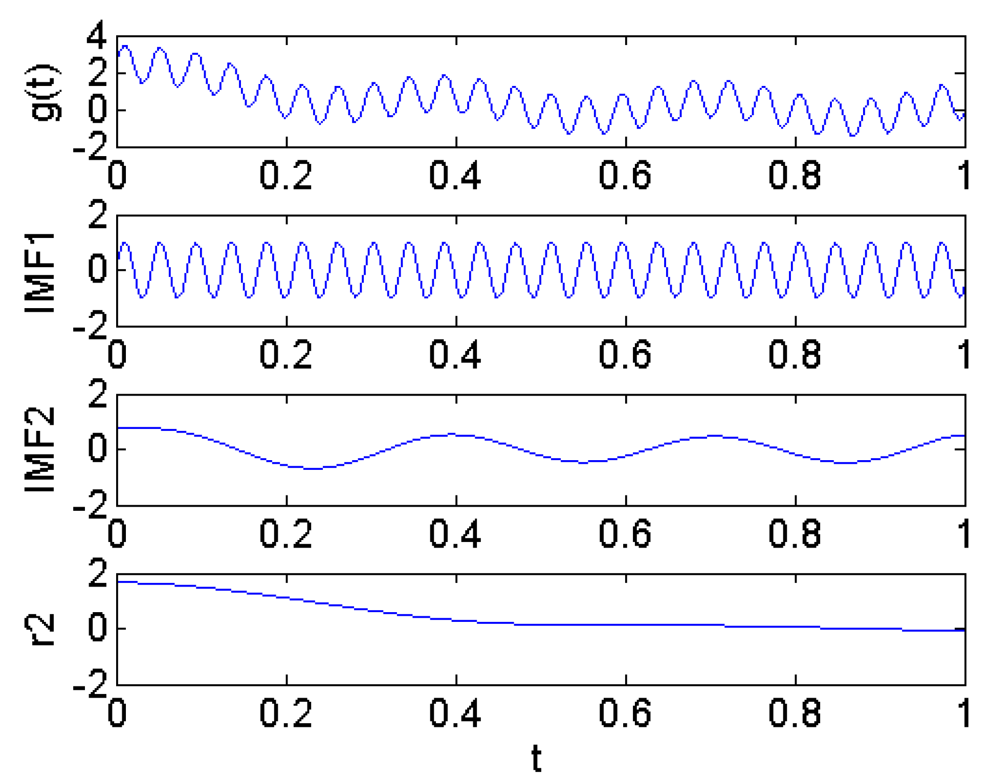
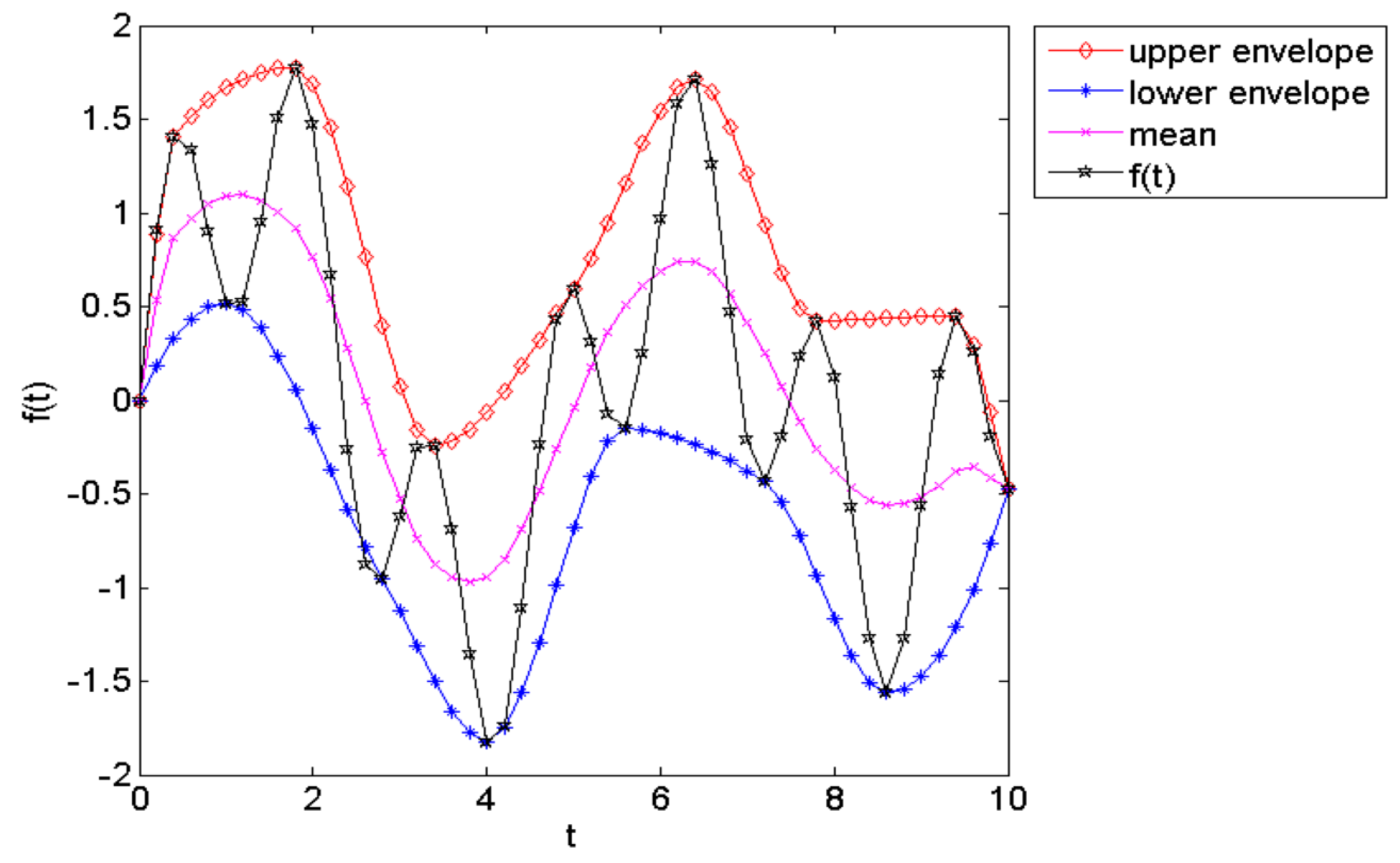
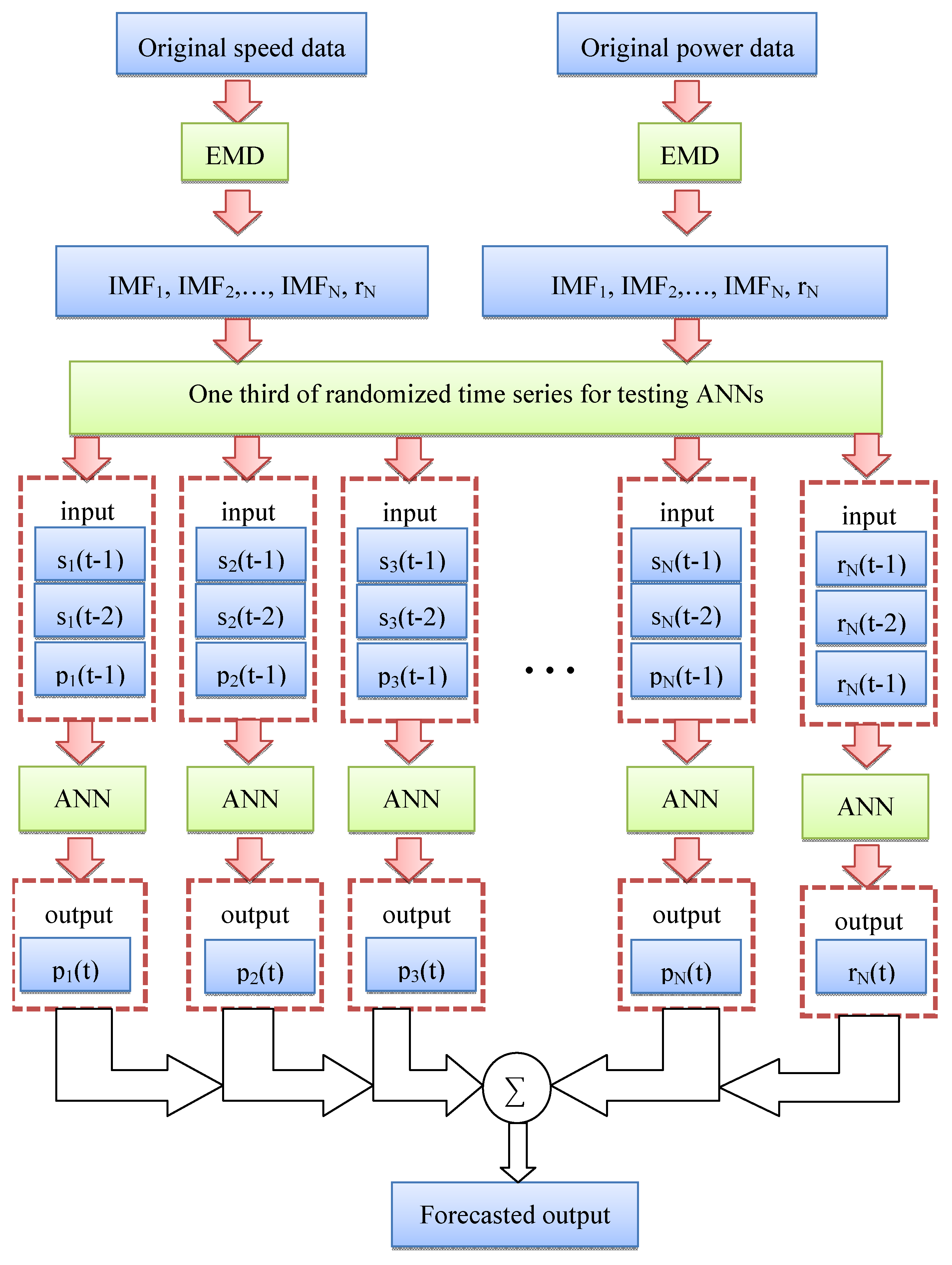
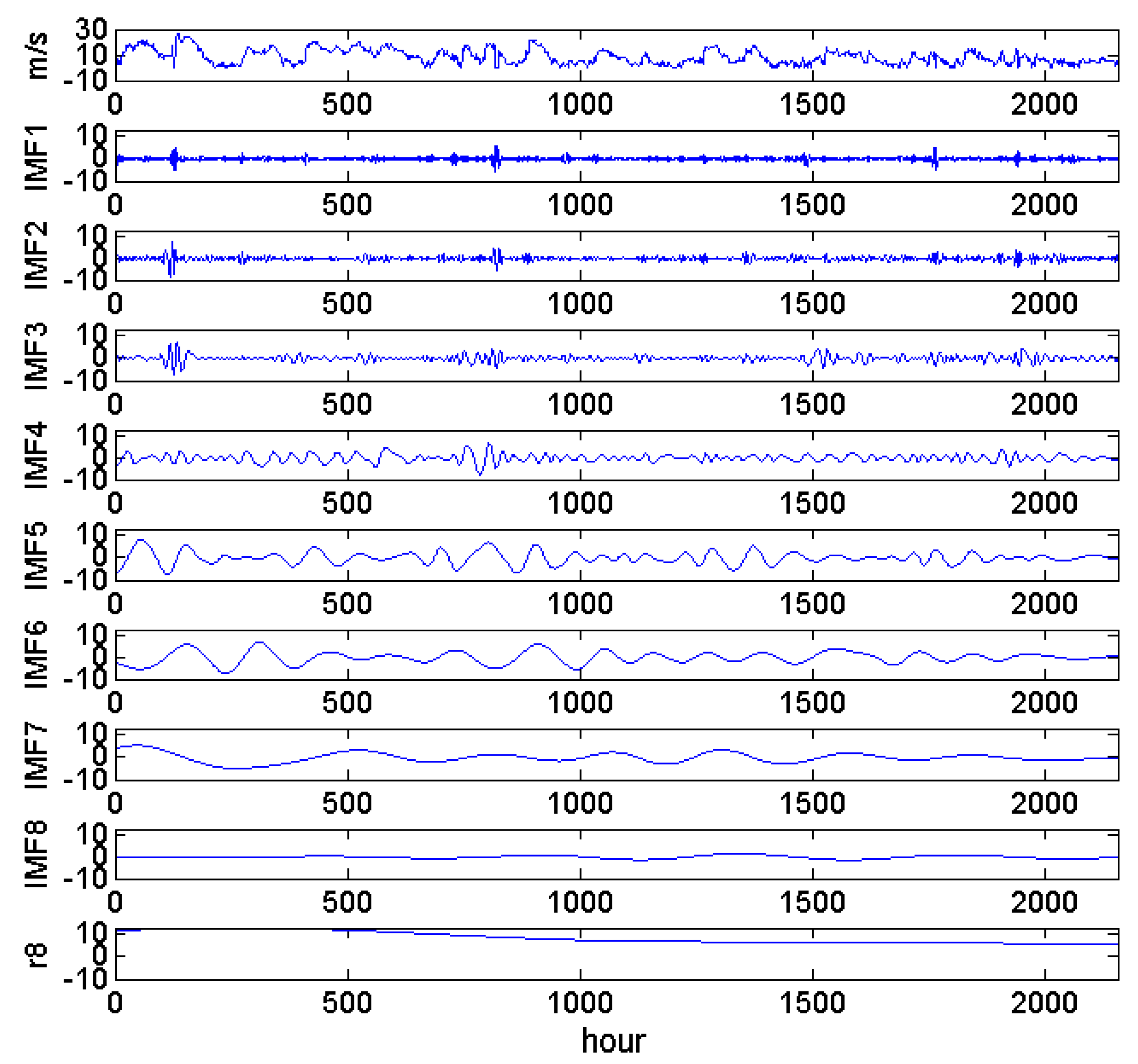
Based on the above discussion, this paper proposes a novel method that integrates the correlation coefficient, empirical mode decomposition (EMD) [23] and back-propagation-based (BP-based) neural network to conduct the short-term (one hour ahead) wind speed and power forecasting. The correlation coefficient is adopted since short-term forecasting is of concern rather than a long-term investigation. EMD can extract symmetry-like low-order and smooth high-order intrinsic mode functions (IMF) from the original signal. In contrast to multi-resolution analysis in [14], EMD does not need the mother wavelet and can decompose the signal (time-series) with a pre-specified tolerance. Because the attribute of IMF is well-behaved, the forecasting is performed using the relatively simple BP-based neural network rather than the sophisticated neural networks used in [13,14,15,19,22].

The rest of this paper is organized as follows: Section 2 describes the proposed method for forecasting short-term wind power and speed. Section 3 then summarizes the simulation results obtained using real data measured in a wind farm. Conclusions are finally drawn in Section 4.

2. Proposed Method

As described in Section 1, this paper presents a back-propagation-based artificial neural network (BP-based ANN) integrated with empirical mode decomposition (EMD) to forecast short-term (hour ahead) wind speed/power in a wind farm. The wind speed/power time series is decomposed by EMD to produce intrinsic mode functions (IMFs) and a residual function. Mother wavelet and determination of number of scales, which are essential in the multi-resolution analysis of the wavelet transform in [14], are unnecessary. Vital parameters are identified to forecast the hour-ahead wind speed/power by using the correlation coefficients. Then individual BP-based ANNs are trained using individual IMFs and the residual function. The individual results are achieved by aggregating all forecasted IMFs.

2.1. Correlation Coefficient

An individual commercial wind turbine has its well-defined power curve which presents the power output versus the wind speed impinging on its rotor. However, this power curve cannot be used directly for the power output of a wind turbine in a wind farm because of: (i) the layout of multiple wind turbines in a wind farm; (ii) different rotor speed control techniques resulting in various tip-speed ratios; (iii) height of the anemometer; (iv) cut-in/cut-off wind speeds; and (v) turbulence in a wind farm. Consequently, this paper considers the most essential factor (i.e., wind speed) to correlate the power output of a wind turbine in a wind farm. This section describes how to evaluate the correlation between the wind speeds and wind powers at different times. Because the short-term forecasting is concerned, the correlation coefficient in statistics is adopted herein. More specifically, assume that $x_1,x_2,x_3,\mathrm{...}\text{, }{x}_n$ and $y_1,y_2,y_3,\mathrm{...}\text{, }{y}_n$ are two sets of sampling data. Let their mean values be $\overline{x}$ and $\overline{y}$, respectively. Their standard deviations are denoted as S_x and S_y. The correlation coefficient is then defined as follows:

$$R_{xy}=\frac{S_{xy}}{S_x{S}_y}=\frac{{\displaystyle \sum _{i=1}^n(x_i-\overline{x})(y_i-\overline{y})}}{\sqrt{{\displaystyle \sum _{i=1}^n{(x_i-\overline{x})}^2}}\sqrt{{\displaystyle \sum _{i=1}^n{(y_i-\overline{y})}^2}}}$$

(1)

Equation (1) expresses the correlation between these two samples. The values of R_xy are within [−1, 1]. If |R_xy| < 0.4, the correlation of these two samples is low. Generally, if 0.7 ≤ |R_xy| < 1, these two sets of samples are correlated with each other. For most applications, an absolute value of R_xy greater than 0.8 is requested to ensure that two sample sets are highly correlated with each other.

2.2. Empirical Mode Decomposition

As described in Section 1, the wind speed and wind power are nonlinear and non-stationary time series. Thus, an efficient signal processing technique is required to analyze these time series. Rather than the wavelet transform which needs a mother wavelet, this paper adopts Hilbert-Huang transform (HHT) [23]. HHT is a time-frequency analysis method applicable to non-linear and non-stationary signals. HHT comprises Hilbert spectral analysis (HSA) and empirical mode decomposition (EMD). HHT employs the EMD method to decompose a signal into so-called intrinsic mode function (IMF), and uses the HSA method to obtain instantaneous frequency data. In contrast to the wavelet transform, HHT does not require a priori knowledge of mother wavelet before signal processing.

A signal (time series) can be decomposed into many IMFs through the EMD. Each IMF comprises parts of vital features of the signal. Each IMF has two properties [23]:

• The numbers of zero-crossing points, local maxima and minima must be identical or differ from each other at most by one in the whole sampled points;
• The mean of the envelopes defined by the local maxima and minima must equal zero at any point of the signal.

Figure 1 shows the definitions of a signal f(t) and its corresponding mean, upper envelope and lower envelope. Each IMF can have varying amplitudes and frequencies along the t (or time) axis, unlike the traditional Fourier series with individual fixed amplitude and frequency in a harmonic component. Each IMF represents a simple oscillatory mode.

Figure 1. A signal f(t) and its mean, upper and lower envelopes.

Figure 1. A signal f(t) and its mean, upper and lower envelopes.

Extracting an IMF from a signal f(t) is referred to as sifting. EMD can be performed by two iterative loops. Let i and j denote the outer and inner iteration indices, respectively. The outer loop is designed to find the i-th intrinsic mode function. The inner loop includes iterations to evaluate an intrinsic mode function. First, all local maxima and minima of the signal f_ij(t) are located and then these maxima and minima are interpolated to attain the upper and lower envelopes, respectively, by the cubic spline curve fitting. If a predefined convergence criterion is met, then an IMF is attained by calculating IMF_i(t) = f_ij(t) − m_ij(t) where m_ij(t) is the mean of the upper and lower envelopes. In the meanwhile, a residual function r_i(t) is gained by computing f_i1(t) − IMF_i(t). If the convergence criterion is not fulfilled, then new local maxima, minima and mean of f_ij(t) − m_ij(t) are calculated. The outer loop stops if r_i(t) satisfies a predefined termination criterion.

Thus, the signal f(t) can be decomposed and expressed by Equation (2). Restated, a time-series function f(t) can be expressed in terms of the sum of Nc IMFs and one residue r_Nc(t):

$$f(t)={\displaystyle \sum _{i=1}^{Nc}IM{F}_i(t)+r_{Nc}(t)}$$

(2)

In this paper, f(t) signifies the wind speed or power time-series. Each time series is decomposed into some IMF_i(t) where i = 1, 2, 3, …, Nc, plus a residue r_Nc(t). The term Nc is the number of IMFs. The value of Nc is determined by the termination criterion.

Nc plus one ANNs are needed to conduct the short-term wind speed/power forecasting by taking the Nc IMFs wind speed/power time series and their residual functions into account. However, there are two reasons for one not to utilize the entire Nc IMFs and residual function as follows: (i) the computational complexity should be reduced and (ii) high-order IMFs are smooth. Thus, the following decomposition is considered:

$$f(t)={\displaystyle \sum _{i=1}^{N}IM{F}_i(t)+r_N(t)}$$

(3)

where N equals round(Nc/2) + 1 and the symbol “round(•)” refers to round-off. The new residual function can be evaluated as follows:

$$r_N(t)={\displaystyle \sum _{i=N+1}^{Nc}IM{F}_i(t)+r_{Nc}(t)}$$

(4)

Alternatively, the maximum number of outer iterations can be set to N and r_N(t) can be gained once the algorithm process stops. Figure 2 illustrates a function g(t) = sin(150t) + 0.5 × sin(20t) + 2.5 × exp(−5t) that can be decomposed into IMF₁, IMF₂ and a residual function r₂(t).

Figure 2. A function g(t) and its intrinsic mode functions (IMF₁ and IMF₂) and residual function (r₂).

Figure 2. A function g(t) and its intrinsic mode functions (IMF₁ and IMF₂) and residual function (r₂).

Thus, the number of ANNs to forecast the wind power/speed is significantly reduced from Nc to N. Simulation results indicate that the accuracy of the proposed method still remains. Notably, no heuristic setting or a priori assumption is required, e.g., given the mother wavelet in the wavelet transform.

2.3. Back-Propagation-Based Neural Network

The purpose of ANN serves as a block box that is used to correlate the forecasted “intrinsic wind speed” and “intrinsic wind power” to the preceding “intrinsic wind speed” and “intrinsic wind power”. The numbers of preceding “intrinsic wind speed” and “intrinsic wind power” are determined by the correlation coefficients in Section 2.1. BP-based ANN rather than complex ANNs are used in this work for the following reasons:

• The studied wind power (speed) time-series has been decomposed into N IMFs and one residual function. Each IMF becomes less nonlinear and non-stationary.
• The numbers of input and output neurons are not large, i.e., 20 (maximum) and 1, respectively.

Let η and κ denote the seasons (spring, summer, autumn and winter) and targets (speed or power) indices, respectively. For example, a BP-based ANN is used to forecast pi(t) using pi(t − 1), pi(t − 2), pi(t − 3), …, pi(t − T1(η,κ)) and si(t − 1), si(t − 2), si(t − 3), …si(t − T2(η,κ)), where pi(t) and si(t) denote the “intrinsic wind power” and “intrinsic wind speed” expressed by the IMF for the wind power and speed, respectively. T1(η,κ)and T2(η,κ) are determined by the correlation coefficient. In total, there are (${\displaystyle {\sum }_{\eta =1}^4{\displaystyle {\sum }_{\kappa =1}^{2}N(\eta ,\kappa )+8}}$) BP-based ANNs for the studied wind speed and power data. Independent calculation and forecasting are carried out by each BP-based ANN.

2.4. Algorithmic Stages

The proposed method can be categorized into four stages: (I) data prescreening; (II) EMD for wind speed and power in four seasons; and (III) ANN training; and (IV) ANN testing.

The data prescreening stage evaluates the correlation coefficients of the wind speed and power in the same season. The essential parameters serving as inputs for an ANN are identified. Restated, Equation (1) is applied to evaluate the correlation coefficients of the original wind speed/power time-series in order to determine the number of inputs p_i(t − 1), p_i(t − 2), p_i(t − 3), …, p_i(t − T1(η,κ)) and that of s_i(t − 1), s_i(t − 2), s_i(t − 3), …, s_i(t − T2(η,κ)) to forecast p_i(t) and s_i(t) where the symbol i is the index of the intrinsic mode function.

In the EMD stage, eight sets of wind power and speed in four seasons are studied. In total, ${\displaystyle {\sum }_{\eta =1}^4{\displaystyle {\sum }_{\kappa =1}^{2}N(\eta ,\kappa )}}$ IMFs and eight residual functions are attained.

The ANN training stage deals with eight sets of (N(η,κ) + 1) BP-based ANNs independently. The input-output pairs obtained from each IMF or the residual function are randomly used to train its corresponding ANN. Two-thirds of the whole data are utilized in this stage.

The ANN testing stage takes advantage of trained BP-based ANNs to forecast the wind speed or power in a season. Again, eight sets of (N(η,κ) + 1) BP-based ANNs are studied independently. The final result in a season are achieved by aggregating the individual results obtained by the (N(η,κ) + 1) BP-based ANNs. The remaining one third of the whole data are utilized in this stage.

Figure 3 schematically depicts the ANN testing stage. More specifically, assume that the wind power forecasting and a certain season are considered. For simplification, assume that the identified parameters are p_i(t − 1), s_i(t − 1) and s_i(t − 2) for use in forecasting p_i(t) in Figure 3. That is, T1(η,κ) = 1 and T2(η,κ) = 2. The numbers of input and output neurons of the BP-based ANN are 3 and 1, respectively. The final forecasted wind power in this season is gained by adding all forecasted p_i(t) and r_N(t), where i = 1, 2, …, N.

Figure 3. pi(t) forecasting using identified parameters at times t-1 and t-2 as inputs in the ANN testing stage.

Figure 3. pi(t) forecasting using identified parameters at times t-1 and t-2 as inputs in the ANN testing stage.

3. Results and Discussion

This paper incorporates the use of hour-based measurements including wind power generation from a wind farm and the wind speed from an anemometer. With both taken at the same site in Penghu, Taiwan, these measurements are used to demonstrate the applicability of the proposed method. The wind farm has eight wind generators with an individual capacity size of 600 kW. A set of 24 × 365 data (1 December 2003, through 30 November 2004) is employed in the studies.

3.1. Identification of Critical Parameters Using Correlation Coefficients

A large correlation coefficient R_xy, e.g., 0.8, implies a high correlation between the two studied data sets. As shown in Table 1, the numbers of P(t − n), n = 1, 2, 3, … highly related to P(t) are 5, 8, 10 (maximum) and 4 for spring, summer, autumn and winter, respectively. Furthermore, the numbers of S(t − n), n = 1, 2, 3, … highly related to P(t) are 4, 6, 10 and 1 for the spring, summer, autumn and winter, respectively (see Table 2). Thus, the numbers of input neurons of the BP-based ANNs for these four seasons are 9, 14, 20 and 5, respectively.

Table 1. Correlation coefficients between two wind power time series (t is the index for hours).

Relations	Correlation coefficients
	Spring	Summer	Autumn	Winter
P(t − 1) to P(t)	0.96	0.95	0.98	0.93
P(t − 2) to P(t)	0.92	0.92	0.96	0.88
P(t − 3) to P(t)	0.88	0.89	0.95	0.85
P(t − 4) to P(t)	0.85	0.86	0.93	0.82
P(t − 5) to P(t)	0.82	0.84	0.92	0.79
P(t − 6) to P(t)	0.80	0.83	0.91	0.77
P(t − 7) to P(t)	0.77	0.81	0.90	0.74
P(t − 8) to P(t)	0.74	0.80	0.89	0.72
P(t − 9) to P(t)	0.72	0.79	0.88	0.71
P(t − 10) to P(t)	0.69	0.78	0.870	0.68

Table 1. Correlation coefficients between two wind power time series (t is the index for hours).

Relations	Correlation coefficients
	Spring	Summer	Autumn	Winter
P(t − 1) to P(t)	0.96	0.95	0.98	0.93
P(t − 2) to P(t)	0.92	0.92	0.96	0.88
P(t − 3) to P(t)	0.88	0.89	0.95	0.85
P(t − 4) to P(t)	0.85	0.86	0.93	0.82
P(t − 5) to P(t)	0.82	0.84	0.92	0.79
P(t − 6) to P(t)	0.80	0.83	0.91	0.77
P(t − 7) to P(t)	0.77	0.81	0.90	0.74
P(t − 8) to P(t)	0.74	0.80	0.89	0.72
P(t − 9) to P(t)	0.72	0.79	0.88	0.71
P(t − 10) to P(t)	0.69	0.78	0.870	0.68

Table 2. Correlation coefficients between wind power and speed time-series (t is the index for hours).

Relations	Correlation coefficients
	Spring	Summer	Autumn	Winter
S(t − 1) to P(t)	0.91	0.90	0.88	0.81
S(t − 2) to P(t)	0.88	0.88	0.88	0.78
S(t − 3) to P(t)	0.85	0.85	0.87	0.76
S(t − 4) to P(t)	0.82	0.83	0.86	0.74
S(t − 5) to P(t)	0.80	0.82	0.85	0.73
S(t − 6) to P(t)	0.77	0.80	0.84	0.71
S(t − 7) to P(t)	0.75	0.79	0.83	0.70
S(t − 8) to P(t)	0.73	0.78	0.83	0.69
S(t − 9) to P(t)	0.70	0.77	0.82	0.68
S(t − 10) to P(t)	0.68	0.76	0.81	0.66

Table 2. Correlation coefficients between wind power and speed time-series (t is the index for hours).

Relations	Correlation coefficients
	Spring	Summer	Autumn	Winter
S(t − 1) to P(t)	0.91	0.90	0.88	0.81
S(t − 2) to P(t)	0.88	0.88	0.88	0.78
S(t − 3) to P(t)	0.85	0.85	0.87	0.76
S(t − 4) to P(t)	0.82	0.83	0.86	0.74
S(t − 5) to P(t)	0.80	0.82	0.85	0.73
S(t − 6) to P(t)	0.77	0.80	0.84	0.71
S(t − 7) to P(t)	0.75	0.79	0.83	0.70
S(t − 8) to P(t)	0.73	0.78	0.83	0.69
S(t − 9) to P(t)	0.70	0.77	0.82	0.68
S(t − 10) to P(t)	0.68	0.76	0.81	0.66

3.2. Empirical Mode Decomposition and Residual Functions

Figure 4 shows the EMD of wind speed during the spring, including eight IMFs and one residual function (r₈). The original wind speed is volatile which is non-stationary and inappropriate for use of ANN to explore. Based on Figure 4, we can infer the following:

(i)

Although the wind speeds are positive, the values of IMFs may be negative;

(ii)

The values of IMF₁~IMF₃ oscillate with high frequencies and are nearly symmetrical. Owing to this phenomenon, a BP-based ANN can forecast the future LMPs properly;

(iii)

The values of IMF₄~IMF₆ vary slowly and still remain approximately symmetrical. Based on this condition, a BP-based ANN is able to work easily; and

(iv)

The values of IMF₇, IMF₈ and r₈ alter gradually and smoothly. A BP-based ANN again functions without any difficulty under this circumstance.

Figure 4. Empirical mode decomposition of wind speed in the spring.

Figure 4. Empirical mode decomposition of wind speed in the spring.

As mentioned earlier in Section 2, the signal does not need to be extracted into many IMFs. In this case, Nc = 8. This proposed method suggests that the number of essential IMFs is around (8/2)+1, i.e., 5. Therefore, the wind speed time-series during the spring is expressed by:

$$S(t)={\displaystyle \sum _{i=1}^{5}IM{F}_i(t)+r_5(t)}$$

(5)

The new residual function can be evaluated as follows:

$$r_5(t)={\displaystyle \sum _{i=6}^{8}IM{F}_i(t)+r_8(t)}$$

(6)

Alternatively, the outer iteration can be performed five times and the remaining function is r₅(t). Whether or not the values of new residual function still vary slowly and smoothly should be examined. If the new residual function is no more volatile, the simple BP-based ANN can definitely work perfectly. Figure 5 shows the new residual functions of wind speeds (m/s) during the four seasons. These new residual functions reveal that the “residual” wind speeds do not significantly vary and the simple BP-based ANN may be applied. Similarly, Figure 6 illustrates new residual functions of wind power (kW) during the four seasons. The same inference for the wind power can be made. Table 3 shows the number (Nc) of IMFs extracted from the original wind speed and power time series.

Figure 5. New residual functions of wind speeds (m/s) during the four seasons: (a) spring; (b) summer; (c) autumn; and (d) winter.

Figure 5. New residual functions of wind speeds (m/s) during the four seasons: (a) spring; (b) summer; (c) autumn; and (d) winter.

Figure 6. New residual functions of wind powers (kW) during the four seasons: (a) spring; (b) summer; (c) autumn; and (d) winter.

Figure 6. New residual functions of wind powers (kW) during the four seasons: (a) spring; (b) summer; (c) autumn; and (d) winter.

Table 3. Numbers of IMFs extracted from the wind power and speed time series during the four seasons.

Seasons	Number of IMFs
	Wind power	Wind speed
Spring	8	8
Summer	10	8
Autumn	11	9
Winter	10	10

Table 3. Numbers of IMFs extracted from the wind power and speed time series during the four seasons.

Seasons	Number of IMFs
	Wind power	Wind speed
Spring	8	8
Summer	10	8
Autumn	11	9
Winter	10	10

3.3. Comparative Studies

The proposed method is achieved by four algorithmic stages presented in Section 2.4. Section 3.1 determines the numbers of input neurons of the BP-based ANNs serving as wind speed/power forecasters during the four seasons (Stage I). Section 3.2 describes the numbers of IMFs, as shown in Table 3, extracted from the wind speed/power time series (Stage II). In Stage III, eight sets of (N(η,κ) + 1) BP-based ANNs are trained independently, as described in Section 2.4. A schematic diagram, as shown in Figure 3, illustrates the method to aggregate the hour-ahead forecasted wind power at time t in Stage IV. A moving data window with a fixed number determined in Stage I is applied to the wind speed/power time series in the forms of IMF or residual function to produce the forecasted wind speed/power at time t.

This section investigates the comparative studies using the proposed method (Nc and N IMFs), traditional BP-based ANN (without EMD), autoregressive integrated moving average (ARIMA) and traditional persistence method. The ARIMA model fits the non-stationary time series data to predict future points in the series (i.e., forecasting). The model is generally referred to as an ARIMA(p,d,q) model where parameters p, d, and q are non-negative integers that refer to the order of the autoregressive, integrated, and moving average parts of the model, respectively. The traditional persistence method assumes that the conditions at the time of the forecast won’t change. The mean absolute error (MAE) and root-mean-squared error (RMSE) act as the performance indices among these five methods. Table 4, Table 5, Table 6 and Table 7 show the MAE and RMSE of forecasted wind speed/power obtained by different methods. Based on these tables, the following comments are made:

(i)

Both MAE and RMSE indicate that the proposed methods with Nc and N IMFs lead to almost the same performance. Thus, N IMFs are sufficient; the computational burden with N IMFs may significantly reduced due to N < Nc;

(ii)

The proposed method nearly has the best performance among these methods while studying eight cases in these seasons;

(iii)

For most of the cases, ARIMA and the persistence method perform better than traditional ANN without EMD.

Table 4. MAE of forecasted wind speed (m/s) obtained by various methods.

Methods	Spring	Summer	Autumn	Winter
ANN & EMD with Nc IMFs	0.59	0.41	0.46	0.90
ANN & EMD with N IMFs	0.58	0.41	0.46	0.90
ANN without EMD	1.25	0.83	0.91	1.02
ARIMA	0.97	0.78	0.81	1.07
Persistence method	0.93	0.79	0.80	0.97

Table 4. MAE of forecasted wind speed (m/s) obtained by various methods.

Methods	Spring	Summer	Autumn	Winter
ANN & EMD with Nc IMFs	0.59	0.41	0.46	0.90
ANN & EMD with N IMFs	0.58	0.41	0.46	0.90
ANN without EMD	1.25	0.83	0.91	1.02
ARIMA	0.97	0.78	0.81	1.07
Persistence method	0.93	0.79	0.80	0.97

Table 5. MAE of forecasted wind power (kW) obtained by various methods.

Methods	Spring	Summer	Autumn	Winter
ANN & EMD with Nc IMFs	27.02	27.50	25.06	36.57
ANN & EMD with N IMFs	27.05	27.47	25.03	36.59
ANN without EMD	34.70	43.71	37.06	36.45
ARIMA	34.87	34.54	26.87	37.30
Persistence method	31.27	35.06	25.00	31.22

Table 5. MAE of forecasted wind power (kW) obtained by various methods.

Methods	Spring	Summer	Autumn	Winter
ANN & EMD with Nc IMFs	27.02	27.50	25.06	36.57
ANN & EMD with N IMFs	27.05	27.47	25.03	36.59
ANN without EMD	34.70	43.71	37.06	36.45
ARIMA	34.87	34.54	26.87	37.30
Persistence method	31.27	35.06	25.00	31.22

Table 6. RMSE of forecasted wind speed (m/s) obtained by various methods.

Methods	Spring	Summer	Autumn	Winter
ANN & EMD with Nc IMFs	1.01	0.66	0.67	2.13
ANN & EMD with N IMFs	1.01	0.66	0.67	2.13
ANN without EMD	2.73	1.31	1.62	2.06
ARIMA	1.62	1.16	1.14	2.10
Persistence method	1.49	1.16	1.17	2.18

Table 6. RMSE of forecasted wind speed (m/s) obtained by various methods.

Methods	Spring	Summer	Autumn	Winter
ANN & EMD with Nc IMFs	1.01	0.66	0.67	2.13
ANN & EMD with N IMFs	1.01	0.66	0.67	2.13
ANN without EMD	2.73	1.31	1.62	2.06
ARIMA	1.62	1.16	1.14	2.10
Persistence method	1.49	1.16	1.17	2.18

Table 7. RMSE of forecasted wind power (kW) obtained by various methods.

Methods	Spring	Summer	Autumn	Winter
ANN & EMD with Nc IMFs	51.01	47.13	41.55	69.87
ANN & EMD with N IMFs	51.03	47.10	41.53	69.86
ANN without EMD	75.35	88.20	66.07	82.72
ARIMA	73.56	60.53	54.99	78.88
Persistence method	68.67	64.75	56.11	81.37

Table 7. RMSE of forecasted wind power (kW) obtained by various methods.

Methods	Spring	Summer	Autumn	Winter
ANN & EMD with Nc IMFs	51.01	47.13	41.55	69.87
ANN & EMD with N IMFs	51.03	47.10	41.53	69.86
ANN without EMD	75.35	88.20	66.07	82.72
ARIMA	73.56	60.53	54.99	78.88
Persistence method	68.67	64.75	56.11	81.37

Figure 7, Figure 8, Figure 9 and Figure 10 show the actual/forecasted wind speeds/powers and errors in four seasons using the proposed method. These figures reveal that the accuracy of wind speed forecasting is indeed very good. The main errors in the wind power forecasting occur when the power generation increases or declines rapidly in the wind-turbine.

Due to activation (transfer) functions in the output neurons of the BP-based ANN, few forecasted results of the wind speeds/powers are negative in Figure 7. To prevent this phenomenon, the activation function may be changed from linear functions to variants of the sigmoid function with positive values. However, the convergence performance of BP-based ANN may become poor. These impractical values are still shown in Figure 7 because MAE and RMSE are evaluated. The negative forecasted value may be modified to be zero and remarked for engineers.

Figure 7. Actual/forecasted wind speeds/powers and errors during the spring: (a) S(t); (b) P(t).

Figure 7. Actual/forecasted wind speeds/powers and errors during the spring: (a) S(t); (b) P(t).

Figure 8. Actual/forecasted wind speeds/powers and errors during the summer: (a) S(t); (b) P(t).

Figure 8. Actual/forecasted wind speeds/powers and errors during the summer: (a) S(t); (b) P(t).

Figure 9. Actual/forecasted wind speeds/powers and errors during the autumn: (a) S(t); (b) P(t).

Figure 9. Actual/forecasted wind speeds/powers and errors during the autumn: (a) S(t); (b) P(t).

Figure 10. Actual/forecasted wind speeds/powers and errors during the winter: (a) S(t); (b) P(t).

Figure 10. Actual/forecasted wind speeds/powers and errors during the winter: (a) S(t); (b) P(t).

4. Conclusions

A novel short-term wind speed and power forecasting method is proposed in this paper. The less nonlinear and non-stationary time series (i.e., intrinsic mode functions) can be extracted through the empirical mode decomposition from the highly volatile wind speed and power. These intrinsic mode functions and its residue are used to train the back-propagation-based artificial neural networks, which serve as a forecaster. Additionally, the concept of residual function is utilized to encompass smooth high-order intrinsic mode functions in order to mitigate the number of artificial neural networks. Complex neural networks are unnecessary since less nonlinear and non-stationary intrinsic mode functions are gained. The individual results are aggregated to achieve the final outcome. A set of realistic measurement, including wind speed and power in one year, are used to validate the accuracy of the proposed method. Simulation results demonstrate that the proposed method performs better than those attained by the conventional neural network, ARIMA and persistence method.

The historical data may be probabilistic or stochastic forms. Thus, a decision making process relying on the forecast may require a probabilistic forecast rather than a deterministic forecast as discussed here. The proposed method can be extended by considering the mean values and standard deviations as two time series. In addition to the mean-value time series, the EMD is also applied to the standard-deviation time series. The numbers of both input and output neurons are doubled.

References

1. National Energy Technology Laboratory. The Modern Grid Strategy. Building a Smart Grid Business Case; A Report Developed for the U.S. Department of Energy, Office of Electricity Delivery and Energy Reliability; National Energy Technology Laboratory: Washington, DC, USA, 2009.
2. Hernández, L.; Baladrón, C.; Aguiar, J.M.; Calavia, L.; Carro, B.; Sánchez-Esguevillas, A.; Sanjuán, J.; González, Á.; Lloret, J. Improved short-term load forecasting based on two-stage predictions with artificial neural networks in a microgrid environment. Energies 2013, 6, 4489–4507. [Google Scholar] [CrossRef]
3. Božić, M.; Stojanović, M.; Stajić, Z.; Tasić, D. A new two-stage approach to short term electrical load forecasting. Energies 2013, 6, 2130–2148. [Google Scholar] [CrossRef]
4. Li, H.Z.; Guo, S.; Zhao, H.R.; Su, C.B.; Wang, B. Annual electric load forecasting by a least squares support vector machine with a fruit fly optimization algorithm. Energies 2012, 5, 4430–4445. [Google Scholar] [CrossRef]
5. Fan, G.F.; Qing, S.; Wang, H.; Hong, W.C.; Li, H.J. Support vector regression model based on empirical mode decomposition and auto regression for electric load forecasting. Energies 2013, 6, 1887–1901. [Google Scholar] [CrossRef]
6. Yoo, J.; Hur, K. Load forecast model switching scheme for improved robustness to changes in building energy consumption patterns. Energies 2013, 6, 1329–1343. [Google Scholar] [CrossRef]
7. Wang, F.; Mi, Z.Q.; Su, S.; Zhao, H.S. Short-term solar irradiance forecasting model based on artificial neural network using statistical feature parameters. Energies 2012, 5, 1355–1370. [Google Scholar] [CrossRef]
8. Ernst, B.; Oakleaf, B.; Ahlstrom, M.L.; Lange, M.; Moehrlen, C.; Lange, B.; Focken, U.; Rohrig, K. Predicting the wind. IEEE Power Energies 2007, 5, 78–89. [Google Scholar] [CrossRef]
9. Barbounis, T.G.; Theocharis, J.B.; Alexiadis, M.C.; Dokopoulos, P.S. Long-term wind speed and power forecasting using local recurrent neural network models. IEEE Trans. Energy Convers. 2006, 21, 273–284. [Google Scholar] [CrossRef]
10. Taylor, J.W.; McSharry, P.E.; Roberto, B. Wind power density forecasting using ensemble predictions and time series models. IEEE Trans. Energy Convers. 2009, 24, 775–782. [Google Scholar] [CrossRef]
11. Bhaskar, K.; Singh, S.N. AWNN-assisted wind power forecasting using feed-forward neural network. IEEE Trans. Sustain. Energy 2012, 3, 306–315. [Google Scholar] [CrossRef]
12. Anastasiades, G.; McSharry, P. Quantile forecasting of wind power using variability indices. Energies 2013, 6, 662–695. [Google Scholar] [CrossRef]
13. Zhang, Q.; Lai, K.K.; Niu, D.X.; Wang, Q.; Zhang, X.B. A fuzzy group forecasting model based on least squares support vector machine (LS-SVM) for short-term wind power. Energies 2012, 5, 3329–3346. [Google Scholar] [CrossRef]
14. Catalão, J.P.S.; Pousinho, H.M.I.; Mendes, V.M.F. Hybrid wavelet-PSO-ANFIS approach for short-term wind power forecasting in Portugal. IEEE Trans. Sustain. Energy 2011, 2, 50–59. [Google Scholar]
15. Potter, C.W.; Negnevitsky, M. Very short-term wind forecasting for Tasmanian power generation. IEEE Trans. Power Syst. 2006, 21, 965–972. [Google Scholar] [CrossRef]
16. Amjady, N.; Keynia, F.; Zareipour, H. Wind power prediction by a new forecast engine composed of modified hybrid neural network and enhanced particle swarm optimization. IEEE Trans. Sustain. Energy 2011, 2, 265–276. [Google Scholar] [CrossRef]
17. Khosravi, A.; Nahavandi, S.; Creighton, D. Prediction intervals for short-term wind farm power generation forecasts. IEEE Trans. Sustain. Energy 2013, 4, 602–610. [Google Scholar] [CrossRef]
18. Li, G.; Shi, J.; Zhou, J.Y. Bayesian adaptive combination of short-term wind speed forecasts from neural network models. Renew. Energy 2011, 36, 352–359. [Google Scholar] [CrossRef]
19. Amjadya, N.; Keyniaa, F.; Zareipour, H. Short-term wind power forecasting using ridgelet neural network. Electric Power Syst. Res. 2011, 81, 2099–2107. [Google Scholar] [CrossRef]
20. Liu, H.; Tian, H.Q.; Chen, C.; Li, Y.F. A hybrid statistical method to predict wind speed and wind power. Renew. Energy 2010, 35, 1857–1861. [Google Scholar] [CrossRef]
21. Jursa, R.; Rohrig, K. Short-term wind power forecasting using evolutionary algorithms for the automated specification of artificial intelligence models. Int. J. Forecast. 2008, 24, 694–709. [Google Scholar] [CrossRef]
22. Zhou, J.Y.; Shi, J.; Li, G. Fine tuning support vector machines for short-term wind speed forecasting. Energy Convers. Manag. 2011, 52, 1990–1998. [Google Scholar] [CrossRef]
23. Huang, N.E.; Shen, Z.; Long, S.R.; Wu, M.C.; Shih, H.H.; Zheng, Q.; Yen, N.C.; Tung, C.C.; Liu, H.H. The empirical mode decomposition and the Hilbert spectrum for nonlinear and nonstationary time series analysis. Proc. R. Soc. Lond. A 1998, 454, 903–995. [Google Scholar] [CrossRef]