1. Introduction
The production of electrical power from wind energy has experienced a remarkable expansion in the last two decades, reaching a total installed capacity of 283 GW in 2012 and growing exponentially at an average annual rate of about 25% [
1,
2]. Considering the large investments being made in the wind energy sector, with many large wind farms being installed and others under planning, optimizing their design and operation is crucial to maximize their performance. Besides maximizing wind farm power output, it is important to understand and predict its variability in order to optimize its integration to the electrical grid. This involves predicting the inherently turbulent atmospheric boundary layer (ABL) flow, its spatial and temporal variability and its interaction with the wind farms. Particularly important is the prediction of multiple turbine wakes, which are known to lead to substantial power losses in wind farms, e.g., [
3,
4,
5,
6,
7,
8,
9].
In wind farms, turbine wake effects on wind velocity deficits and the associated power deficits are modulated by several factors, such as terrain characteristics (e.g., surface roughness, heterogeneity and topography), wind farm characteristics (e.g., turbine type and farm layout) and atmospheric conditions, like wind direction, atmospheric stability and turbulence level. Indeed, changing wind direction can be regarded as changing wind farm layout relative to the incoming wind, while keeping the same turbine density.
Recent field studies [
4,
10] and numerical simulations [
11,
12] have shown that the power deficits in the well-studied Horns Rev offshore wind farm are strongly affected by wind direction for different wind sectors (±1°, ±5°, ±10°, ±15°) around the three selected wind direction angles of
θwind = 270° (from the west), 222° and 312°. For these wind directions, the wind is parallel to different “lines” of wind turbines, leading to what is commonly called full-wake conditions, with different streamwise distances between consecutive turbines (7.0-, 9.3- and 10.5-times the rotor diameter, respectively). In general, the longer that distance, the smaller the wake-induced power losses, particularly in the first rows of turbines. Barthelmie
et al. [
5] reported power data measured at the Horns Rev and the Nysted wind farms for seven wind directions, and showed an obvious increase in the power output from the downwind turbines when the incoming wind angle departs from the full-wake condition. Although all the above-mentioned studies provide valuable insights about the effects of wind direction on power deficits in wind farms, how these effects are related to the turbulent wake flow structure within the farms for a wide range of wind directions (including full-wake and partial-wake conditions) is not yet fully understood.
In this study, large-eddy simulations (LESs) are used to explore the effect of wind direction on the turbine wakes and power output from the Horns Rev wind farm. Particular emphasis is placed on understanding the impact of relatively small changes in wind direction on the wakes and their effect on the total wind farm power generation. The paper is organized as follows:
Section 2 presents the LES framework and describes the different simulation cases. The simulation results are then presented and discussed in
Section 3. Finally, a summary is given in
Section 4.
3. Simulation Results
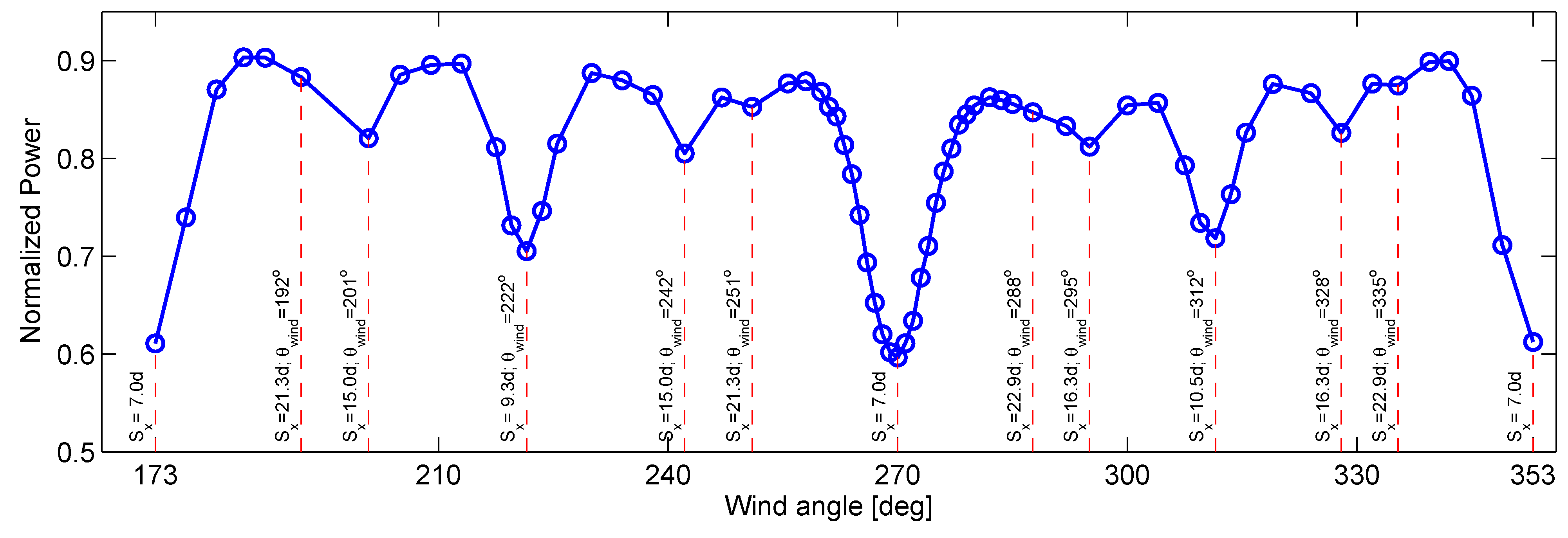
The simulated total power output from the Horns Rev wind farm obtained from the 67 LESs covering a wide range of wind direction angles
θwind (from 173° to 353°), including full-wake and partial-wake conditions, is shown in
Figure 4. Here, and throughout this paper, the simulated power is normalized by the power from an equivalent number of stand-alone wind turbines exposed to the same incoming wind condition. From
Figure 4, it is clear that the minimum wind farm power occurs for the wind directions of 173°, 270° and 353°, which correspond to full-wake conditions with the shortest possible streamwise distance (
Sx = 7.0
d) between consecutive turbines. The farm power output is slightly lower in the 270° case because of the larger number of waked wind turbines in that case (72, compared with 70 for the 173° and 353° cases). Also evident in that figure is the presence of several local minima of power at other wind direction angles [e.g., 201°, 222°, 242° within the south-west (SW) 90° wind sector and 295°, 312°, 328° within the north-west (NW) 90° wind sector], associated with other full-wake conditions with different streamwise distances (
Sx) between consecutive downwind turbines. Some of those wind angles are also illustrated in
Figure 1. It is also interesting to note that relatively higher power outputs are obtained for partial-wake cases in the SW wind sector, compared with those in the NW wind sector. This is due to the fact that, due to its geometry, the wind farm offers a larger frontal area to the wind coming from the SW sector. This larger wind farm frontal area can accommodate a larger number of unwaked turbines, which yields higher power outputs, for specific wind direction angles.
Figure 4.
Distribution of the normalized wind farm power output obtained with large-eddy simulations (LES) for a wide range of wind directions, from 173° to 353°.
Figure 4.
Distribution of the normalized wind farm power output obtained with large-eddy simulations (LES) for a wide range of wind directions, from 173° to 353°.
In order to better understand how the wind direction affects the structure of the multiple turbine wakes inside the farm and, in turn, the wind farm power losses depicted in
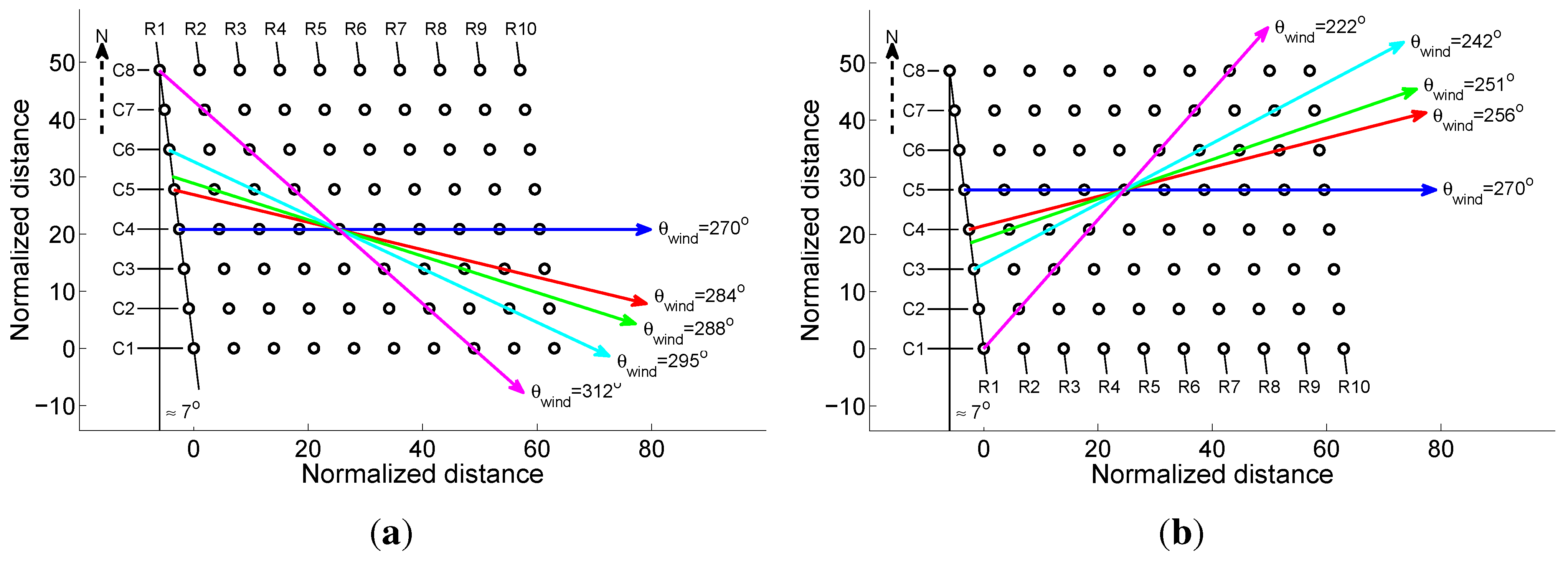
Figure 4, the spatial distribution of the power outputs and the turbine wake flows are analyzed next for five selected cases. They correspond to incoming wind directions of 270°, 284°, 288°, 295° and 312° and are illustrated in
Figure 1a. The distribution of the power output is displayed in
Figure 5, while the turbine wake characteristics, namely, the mean streamwise velocity, vertical velocity, streamwise turbulence intensity and horizontal momentum flux, are shown in
Figure 6,
Figure 7,
Figure 8 and
Figure 9, respectively, for four of those cases. As shown in
Figure 1, all these cases can be considered as full-wake conditions with different streamwise spacings (
Sx) between each wind turbine and its immediately downwind (fully-waked) neighbor. In particular, the streamwise turbine spacing is 7.0
d, 28.9
d, 22.9
d, 16.3
d and 10.5
d for the 270°, 284°, 288°, 295° and 312° cases, respectively. It should be noted that, due to the fixed turbine siting density, an increase in the streamwise turbine spacing leads to a decrease in the spanwise separation between the turbine wake axes. This, in turn, increases the lateral (partial-wake) interactions and, ultimately, the power losses. This explains why, for relatively large
Sx values (larger than about 20.0
d), the differences in power output between full-wake conditions and partial-wake conditions become very small, as depicted in
Figure 4.
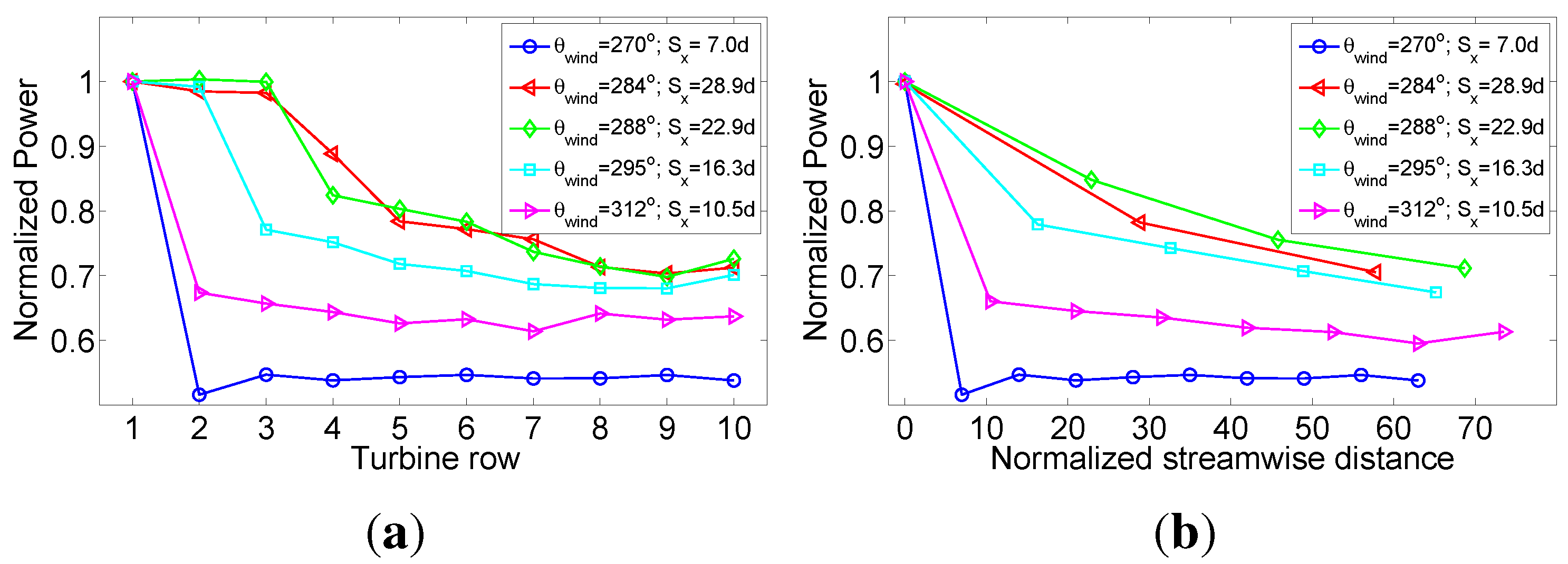
Figure 5.
Spatial distribution of the normalized simulated power output for the five wind angles shown in
Figure 1a: (
a) power output as a function of turbine row (averaged over columns C2, C3 and C4); and (
b) power output distribution along the wind direction lines (lines of turbines) shown in
Figure 1a. The symbols indicate the position of the wind turbines. The streamwise distance is normalized by the turbine rotor diameter
d = 80 m.
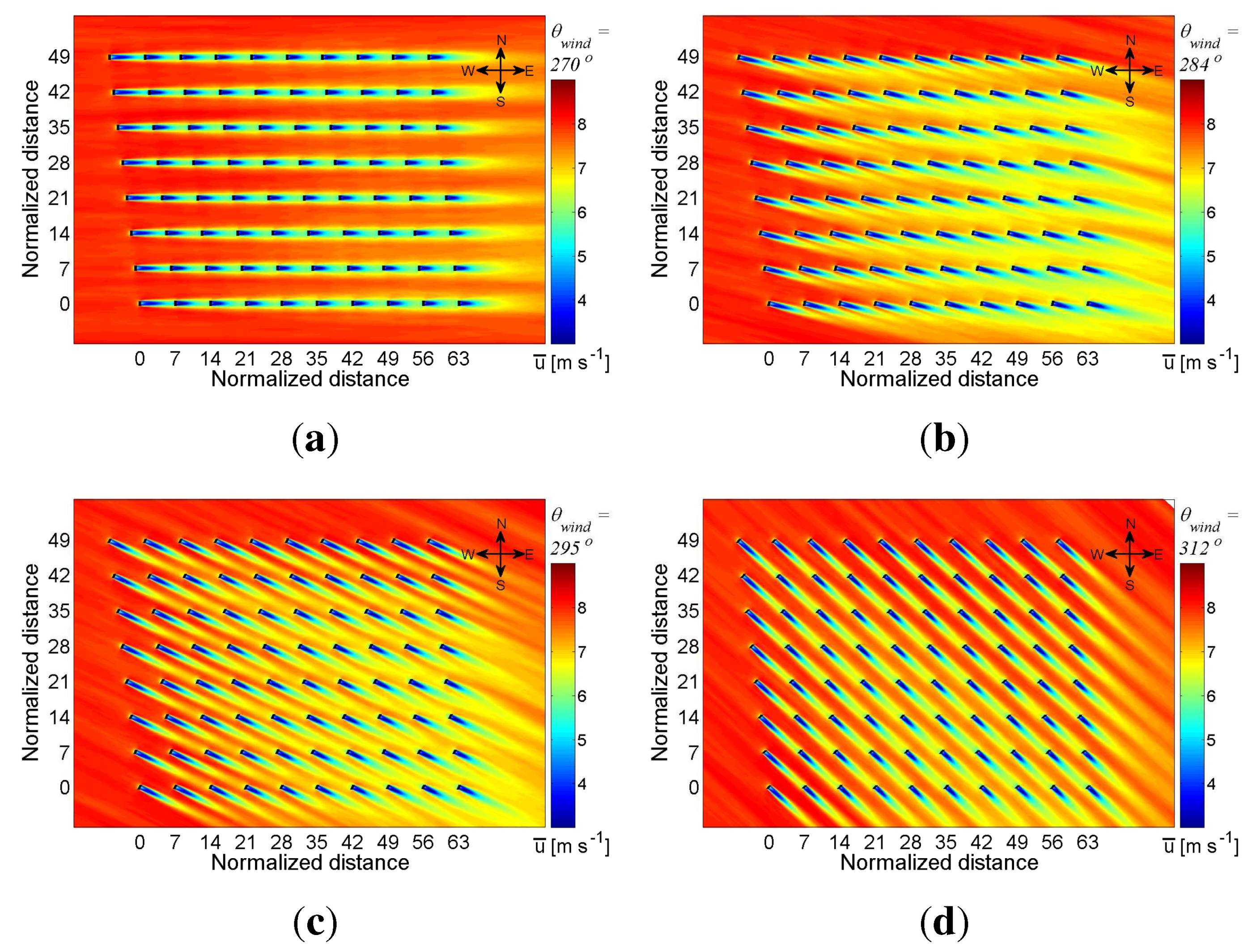
Figure 6.
Contour plot of the time-averaged streamwise velocity on a horizontal plane at hub level for different incoming wind directions of (a) 270°; (b) 284°; (c) 295°; and (d) 312°. Distances are normalized by the turbine rotor diameter d = 80 m.
Figure 6.
Contour plot of the time-averaged streamwise velocity on a horizontal plane at hub level for different incoming wind directions of (a) 270°; (b) 284°; (c) 295°; and (d) 312°. Distances are normalized by the turbine rotor diameter d = 80 m.
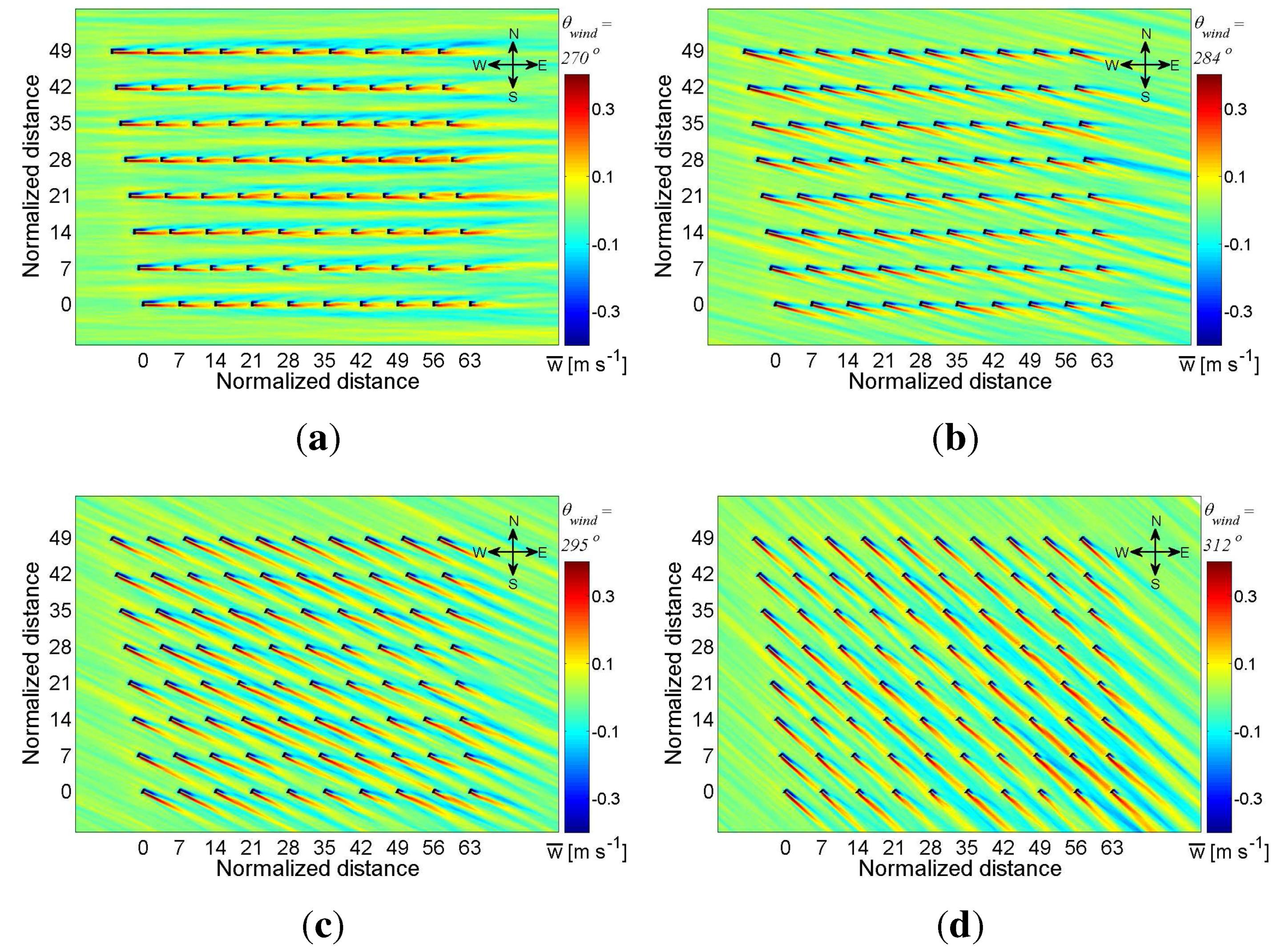
Figure 7.
Contour plot of the time-averaged vertical velocity on a horizontal plane at hub level for different incoming wind directions of (a) 270°; (b) 284°; (c) 295°; and (d) 312°.
Figure 7.
Contour plot of the time-averaged vertical velocity on a horizontal plane at hub level for different incoming wind directions of (a) 270°; (b) 284°; (c) 295°; and (d) 312°.
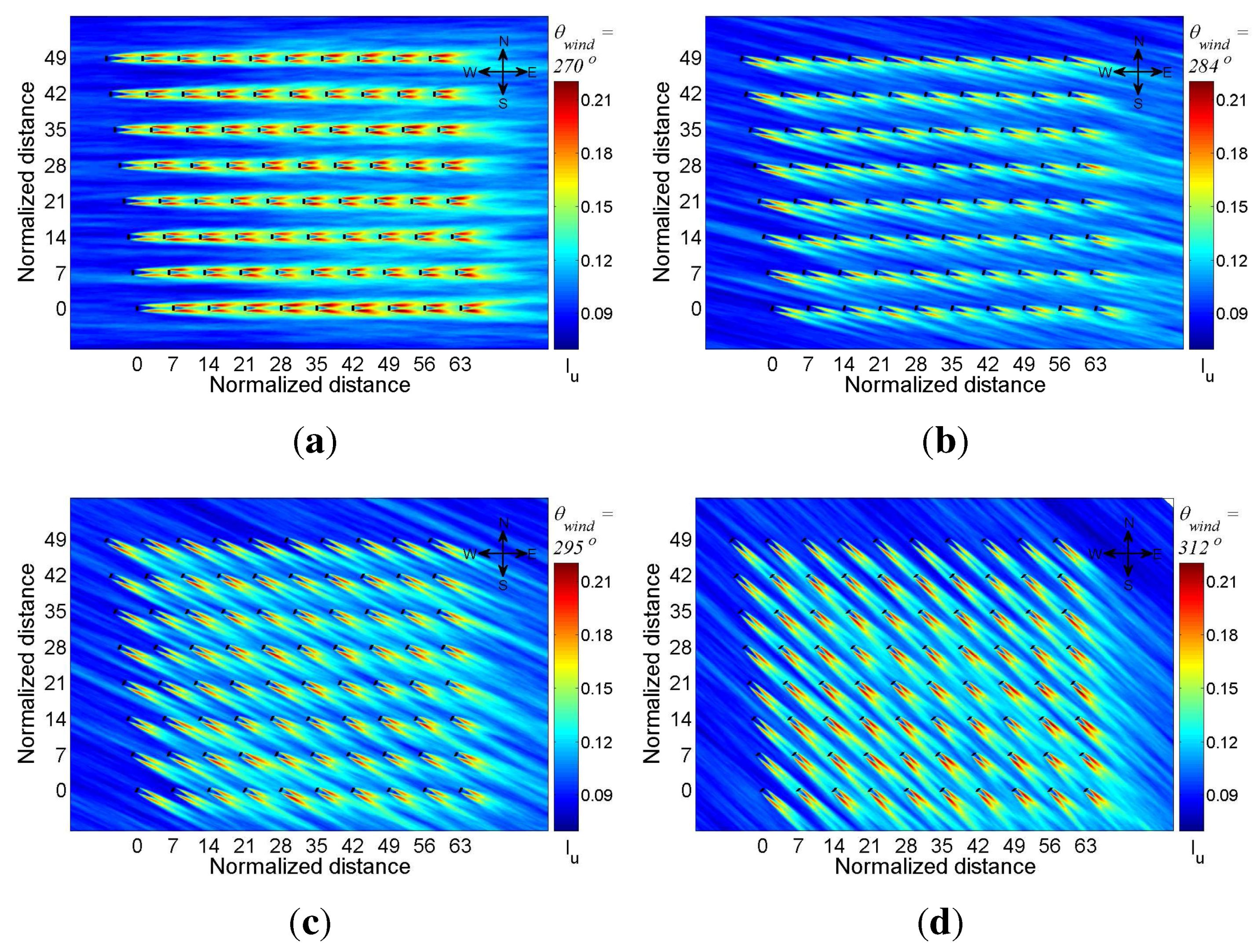
Figure 8.
Contour plot of the streamwise turbulence intensity (resolved part) on a horizontal plane at hub level for different incoming wind directions of (a) 270°; (b) 284°; (c) 295°; and (d) 312°.
Figure 8.
Contour plot of the streamwise turbulence intensity (resolved part) on a horizontal plane at hub level for different incoming wind directions of (a) 270°; (b) 284°; (c) 295°; and (d) 312°.
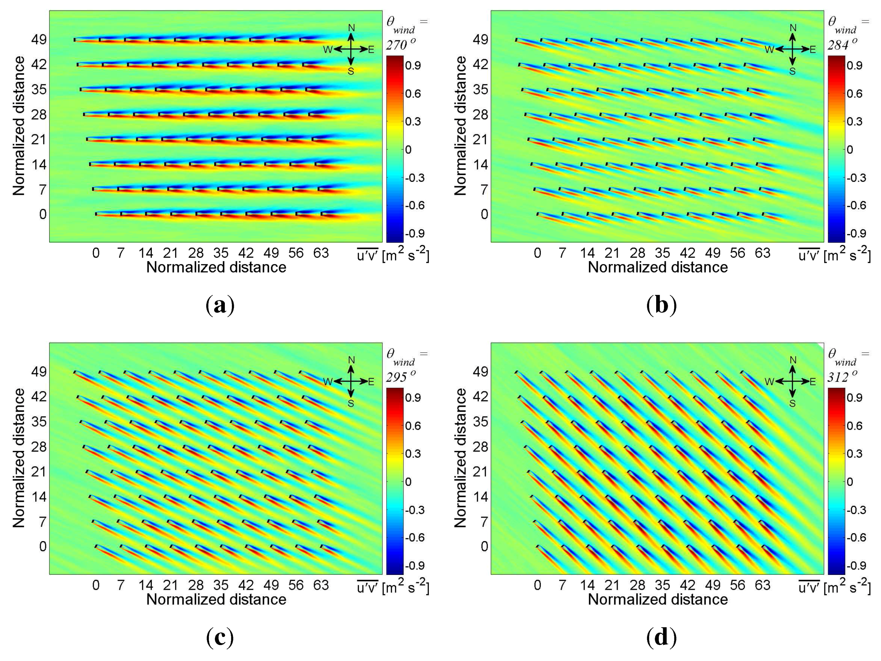
Figure 9.
Contour plot of the horizontal momentum flux [the resolved part plus the subgrid-scale (SGS) part] on a horizontal plane at hub level for different incoming wind directions of (a) 270°; (b) 284°; (c) 295°; and (d) 312°.
Figure 9.
Contour plot of the horizontal momentum flux [the resolved part plus the subgrid-scale (SGS) part] on a horizontal plane at hub level for different incoming wind directions of (a) 270°; (b) 284°; (c) 295°; and (d) 312°.
Figure 5a displays the normalized power output for the five cases under consideration as a function of the turbine row number. The results are obtained by averaging the power output from columns C2 to C4 (see
Figure 1). From these results, it is evident that the spatial distribution of the turbine power output varies greatly with changing wind direction. Consistent with the results for the total farm power output shown in
Figure 4, the largest power deficits throughout the farm are found for the full-wake condition that has the smallest streamwise turbine spacing (
Sx = 7.0
d for
θwind = 270°); it also corresponds to the case of the largest spanwise spacing between lines of turbines (also
Sy = 7.0
d). Here, and throughout this paper, the term ‘line of turbines’ is used to refer to a straight line parallel to the wind direction that connects the hubs of a series of wind turbines under full-wake conditions. It is important to note that, with a small change of wind direction of 14° (from 270° to 284°), the power outputs from all the turbines inside the farm increase substantially, leading to an increment of 43% in normalized wind farm power output (from 0.60 to 0.86), as shown in
Figure 4. There are three reasons that explain this behavior:
The relatively short streamwise distance (
Sx = 7.0
d) between consecutive wind turbines in the 270° case limits the wake recovery, leading to relatively large velocity deficits at the turbine locations (
Figure 6a) and, in turn, large power deficits (see
Figure 5) compared with the other wind direction cases.
The relatively large spanwise distance (
Sy = 7.0
d) between lines of turbines in the 270° case leaves “high-speed channels” (
Figure 6a), inside which a large fraction of the kinetic energy of the incoming wind is convected through the wind farm without being extracted by the turbines. For larger wind direction angles (particularly, 284°), those channels do not exist or are much less evident, thus allowing the wind farm to extract more of the kinetic energy available in the incoming wind.
The wind direction also determines at which row number the turbines begin to be affected by the upwind turbine wakes, which, in turn, defines the total number of waked and unwaked turbines. For example, in the 270° case, a power deficit of about 50% is found already at the second turbine row and affects 90% of the wind farm, while for the 284° case, the first four turbine rows, which make up about 40% of the Horns Rev wind farm, are minimally affected by turbine wakes.
Figure 5b shows the power output from consecutive turbines along the wind directions following the lines shown in
Figure 1. Note that the number of wind turbines in each streamwise row varies from ten to three as the streamwise spacing,
Sx, increases from 7.0
d for 270° to 28.9
d for 284°. In general, the power output from the turbines keeps decreasing along the wind direction. Unlike the 270° case, for which the power output drops sharply at the second turbine row due to the short wake recovery distance (as shown in
Figure 6), and remains nearly constant further downwind, the power reduction is more progressive as one moves downwind inside the wind farm for the other cases with longer streamwise distances between turbines
Sx (particularly for
Sx > 15
d). This can be explained by the fact that the smaller spanwise distance between lines of turbines,
Sy, facilitates lateral wake interactions. The accumulated wakes become wider as they expand downwind (see
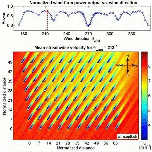
Figure 6), leading to increasingly larger partial-wake effects and, thus, power losses when they interact laterally with the neighboring lines of turbines. In order to further illustrate the effect of wind direction on the turbine-wake structure and associated power losses, the supplementary material contains an animation showing the wind farm power output and the mean streamwise velocity at hub height for all the 67 simulated wind directions (see supplementary material).
Two-dimensional contour plots of the simulated time-averaged vertical velocity component on a horizontal plane at hub height are shown in
Figure 7. The positive and negative vertical velocities obtained on both sides of the wakes highlight the ability of the LES, and in particular of the ADM-R, to reproduce the rotation of the turbine wakes. It should be noted that standard ADMs (without rotation) cannot capture wake rotation because they only account for the thrust force exerted by the turbines. As expected, the wakes rotate in the counter-clockwise direction (for an observer located upwind of the turbine), which is opposite to the standard clockwise rotation of the turbine blades. It should be noted that the vertical velocity distribution in the wakes is non-symmetric, with the positive velocity region extending further downwind compared with the negative velocity. The non-axisymmetry of the wake is a consequence of the interactions of the rotating wake flow with both the land surface and the non-uniform (logarithmic) incoming boundary layer flow. A similar non-axisymmetric distribution of the vertical velocity was reported in simulations of turbine wakes in an on-shore wind farm using the same LES framework [
21].
Figure 8 shows the spatial distribution of the streamwise turbulence intensity inside the wind farm for the same four selected wind directions under consideration. The streamwise turbulence intensity is defined as the ratio between the standard deviation of the local streamwise velocity,
σu, and the mean velocity of the undisturbed inflow at hub height,
. From these results, it is clear that, as expected, turbulence intensity levels are enhanced inside the farm with respect to the incoming wind conditions for all cases. Different wind directions, however, lead to different levels of turbulence enhancement. In particular, the largest turbulence levels at the location of the downwind turbines are found for the 270° case, and they become smaller as the streamwise distance between consecutive turbines increases. Therefore, not only the most severe full-wake cases lead to the strongest velocity deficit and power losses in the wind farm, but they also yield the highest turbulence levels at turbine level and, consequently, the largest fatigue loads on the downwind turbines.
The horizontal turbulent momentum flux, shown in
Figure 9 at hub height, is negative on the right side of the wakes and positive on the left side (looking downwind) for all wind directions. This is consistent with the expected radial flux of momentum towards the wake center, which is associated with entrainment and contributes to the wake recovery. It is interesting to note the non-axisymmetric distribution of the flux, which has a relatively larger magnitude and extends further downwind on the right side, compared with the left side. The magnitude of the radial momentum flux is largest for the cases with the shortest streamwise inter-turbine distance
Sx, which is consistent with the larger turbulence intensities reported in
Figure 8.
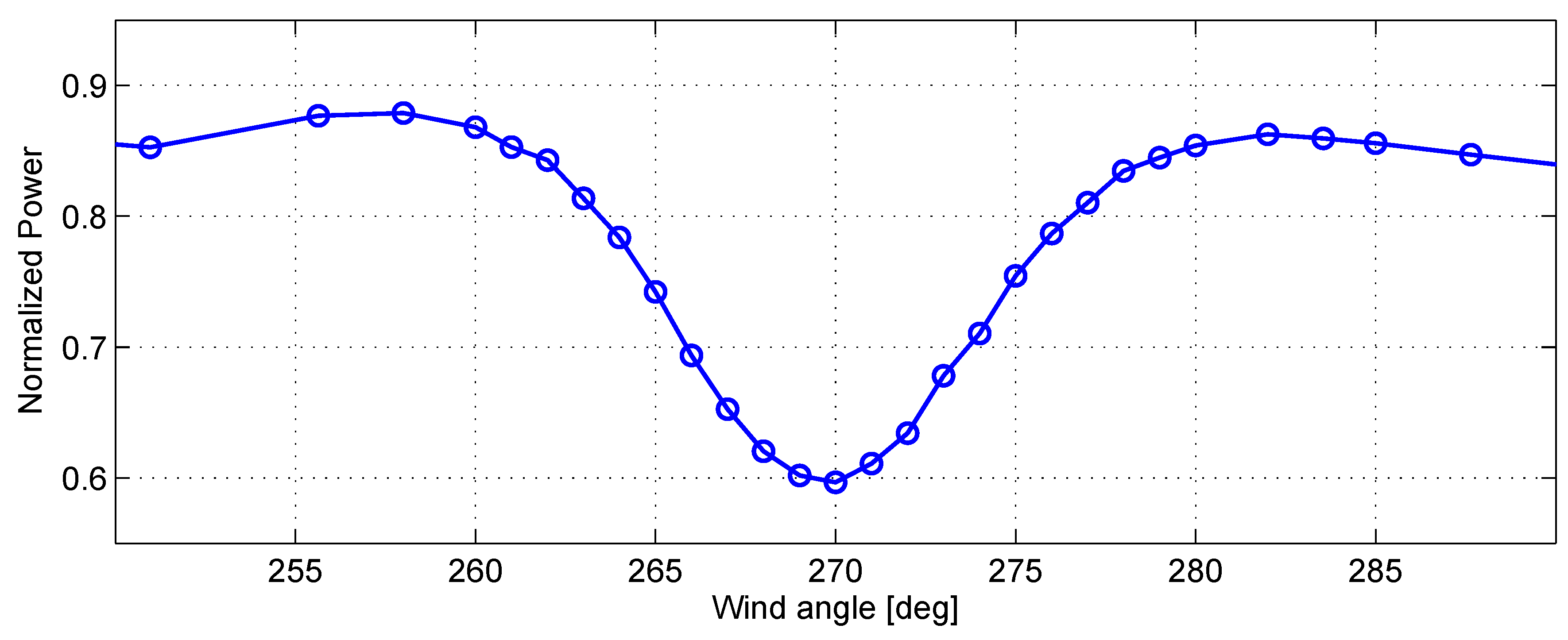
It is important to point out that, as shown in
Figure 10, with a change of wind direction of only 10° from 270°, the total normalized power output from the Horns Rev wind farm increases from its minimum value of 0.60 at 270° to a much higher value of about 0.86 at 270° ± 10°. Overall, these results demonstrate the significant effects that even small changes in wind direction can have on the power output from large wind farms.
Figure 10.
Zoom-in of the total normalized farm power output shown in
Figure 4 for a wind sector between 250° and 290°.
Figure 10.
Zoom-in of the total normalized farm power output shown in
Figure 4 for a wind sector between 250° and 290°.
In order to better understand why a 10° departure from 270° yields such a large increase in power output and why it does not change much for slightly larger wind angles, we compare in
Figure 11 the structure of the wakes for the 280° and 284° wind angles. From this figure, it is evident that, for the 280° wind angle, the turbines are slightly waked by their upwind neighbors in the same row. In the 284° case, the angle difference is just large enough so that the turbines are little affected by the wakes of the immediately upwind turbines.
Figure 11.
Contour plots of the time-averaged streamwise velocity
(m s
−1) around the third, fourth and fifth turbine columns (C3, C4 and C5 in
Figure 1) at hub height for wind angles of (
a)
θwind = 280° and (
b)
θwind = 284°. The black lines show the edge of the wakes (defined using the 1% velocity deficit from the undisturbed flow).
Figure 12.
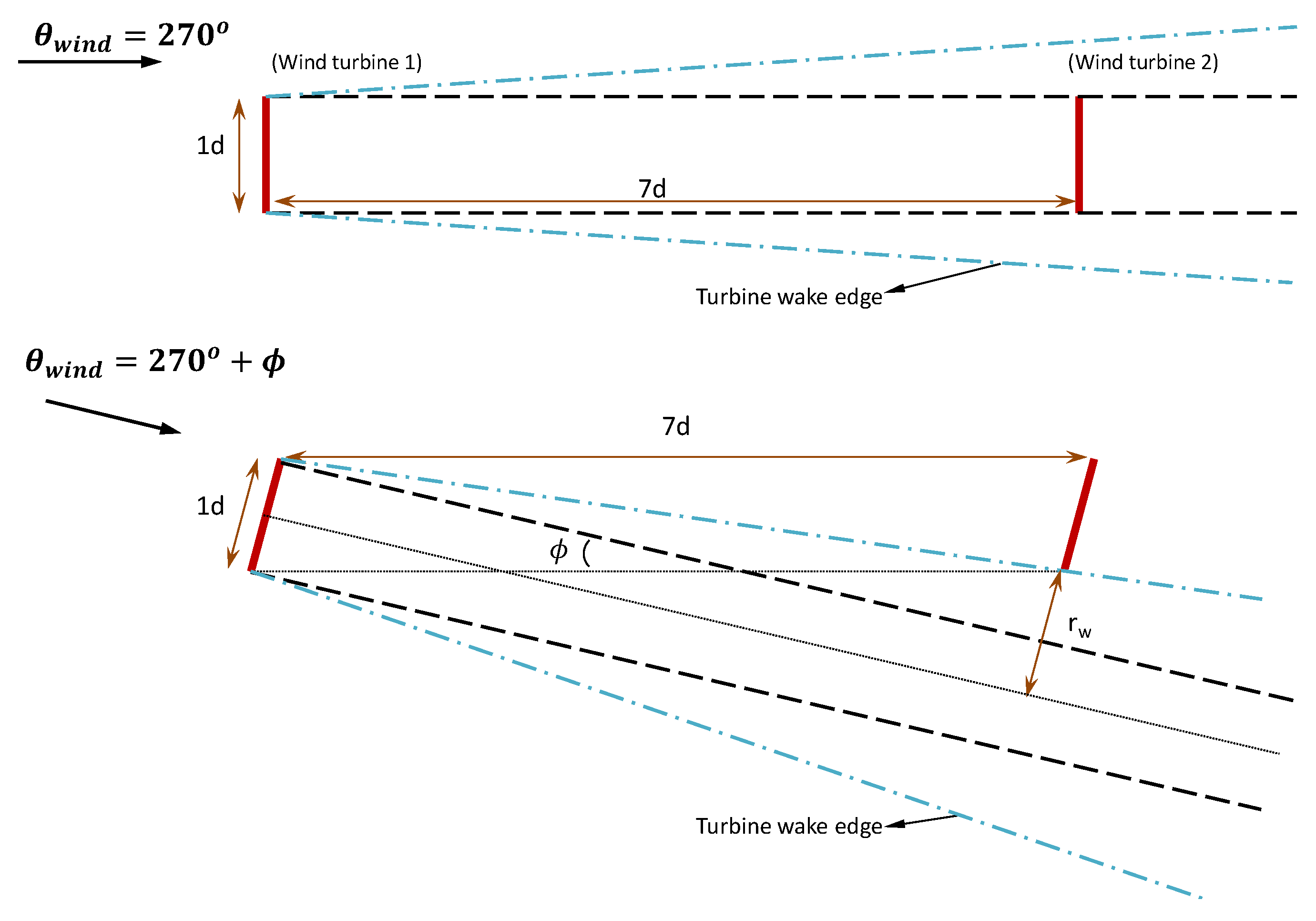
Schematic of the wake from a wind turbine from the first row for two selected wind direction angles: 270°, corresponding to the full wake condition (top); and the minimum angle (270° + ϕ, where ϕ is 14° in this case) required for the wake to have no effect on the next turbine within the same column. The blue dot-dashed line represents the wake edge, and rw is the radius of the wake.
Figure 12.
Schematic of the wake from a wind turbine from the first row for two selected wind direction angles: 270°, corresponding to the full wake condition (top); and the minimum angle (270° + ϕ, where ϕ is 14° in this case) required for the wake to have no effect on the next turbine within the same column. The blue dot-dashed line represents the wake edge, and rw is the radius of the wake.
This finding is in agreement with recent results from LES [
19] and also analytical modeling [
26] that show that, for those inflow conditions (mean velocity and atmospheric turbulence level), the radius of the wake of a stand-alone V-80 turbine expands to reach
rw = 1.2
d (see
Figure 12) at the position of the rotor plane of the second wind turbine at a distance of approximately 6.9
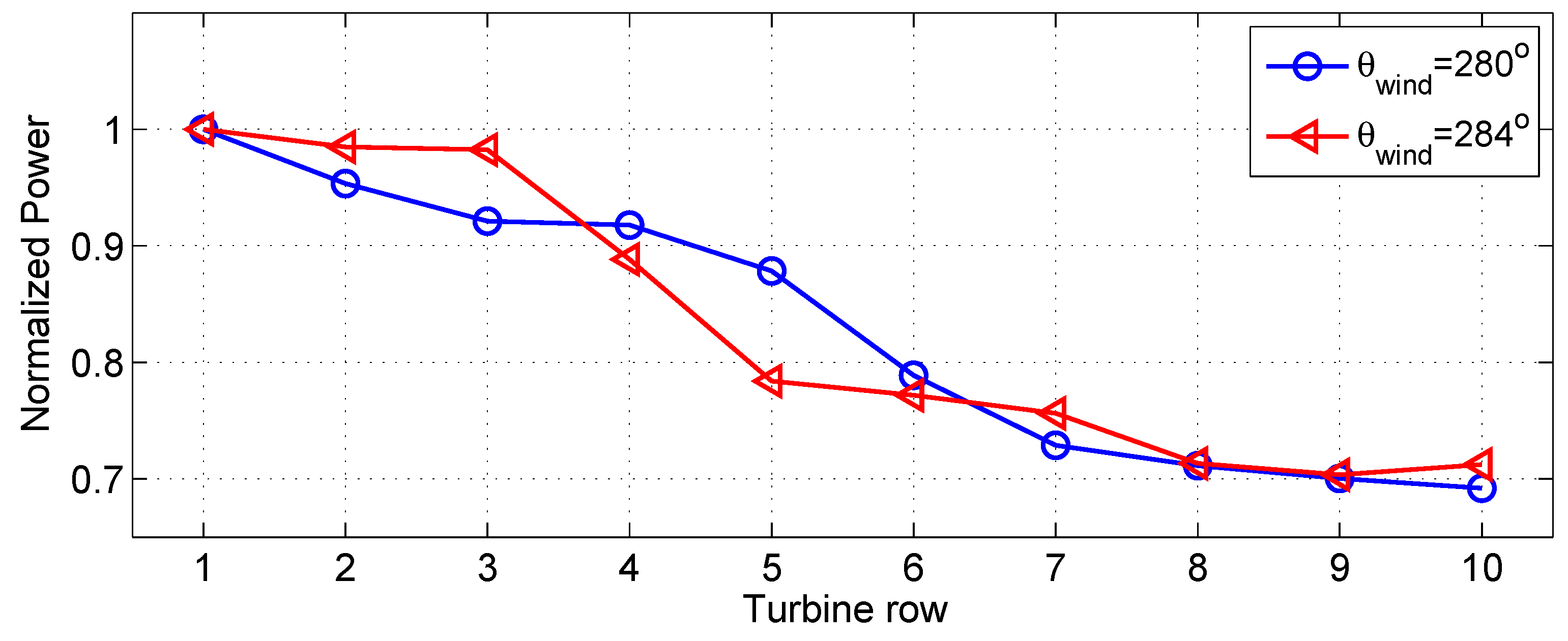
d downwind. In those studies, the turbine wake edge was defined based on the position at which the wake velocity deficit reaches 1% of the incoming wind velocity. That lateral position corresponds to the location of the turbine edge in the 284° case. This explains why the power output from rows 2 and 3 is larger for the 284° wind case compared with the 280° case, for which those rows are affected by partial-wake effects (see
Figure 13). Interestingly, however, this trend is reversed in rows 4–6 (see
Figure 13). This is due to the fact that the larger wind angle increases the effect of the turbine wakes on the neighbor turbine columns, which are affected after the fourth row for
θwind = 284°, while this effect is not evident until the sixth row for the 280° case (see also
Figure 11). The combination of these two opposing wake effects (on the downwind turbines within the same row
vs. on the neighboring turbine columns) makes that, for the layout and size of this wind farm, the two effects cancel out.
Figure 13.
Normalized power output as a function of turbine row for wind angles of
θwind = 280° and
θwind = 284°. The results are averaged over the seven turbine columns (C1 to C7 in
Figure 1).
Figure 13.
Normalized power output as a function of turbine row for wind angles of
θwind = 280° and
θwind = 284°. The results are averaged over the seven turbine columns (C1 to C7 in
Figure 1).
4. Conclusions
LESs were performed to study the effect of wind direction on the power output from a large wind farm. The Horns Rev offshore wind farm was chosen as a case study since the LES code used here was previously validated to predict power output from this farm for some selected wind conditions [
12]. In this recently-developed LES framework [
12,
18,
20,
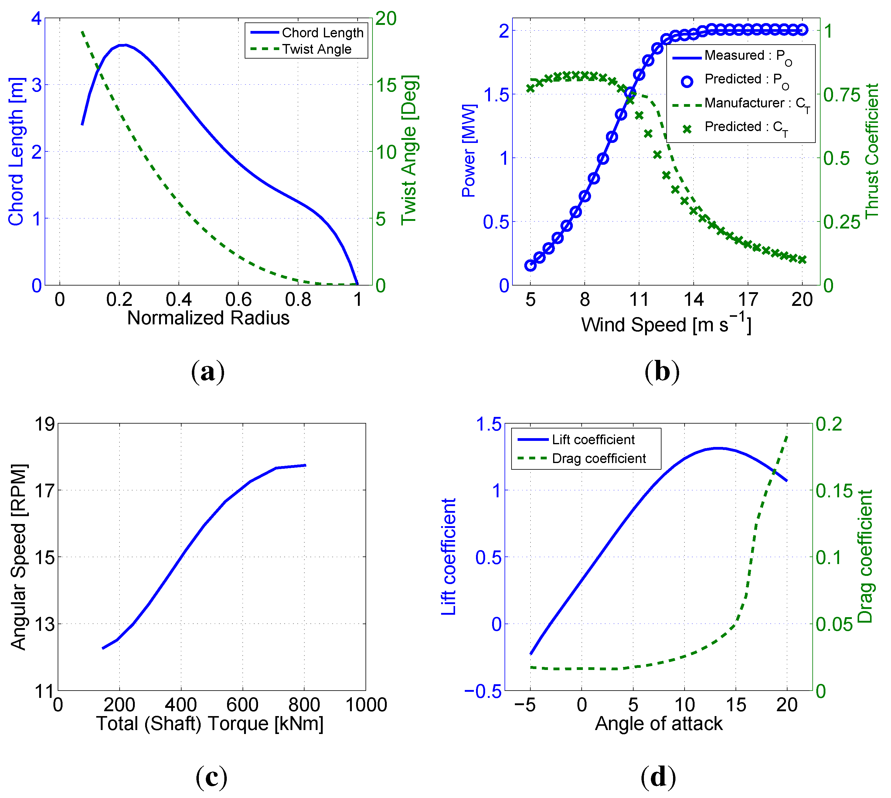
21], the SGS stresses and the turbine-induced forces are parameterized using a tuning-free Lagrangian scale-dependent dynamic model and a dynamic ADM-R, respectively. The dynamic ADM-R couples blade-element theory and a turbine-specific relation between the angular velocity and the shaft torque to compute simultaneously rotor angular velocity, shaft torque and power output.
Simulations with a series of different incoming wind directions show the strong effect of wind direction on the power output from the wind farm. To better understand that variability, it is useful to visualize the changes in wind direction as changes in wind farm layout relative to the mean wind direction, while maintaining the same turbine density (number of turbines per unit area of the farm). In particular, wind direction changes affect the relative separation between wind turbines and their immediately downwind (waked) neighbors, which, in turn, affects the velocity and power deficits. This explains why, for example, the smallest power output corresponds to the full-wake condition associated with the shortest streamwise distance (Sx = 7.0 d) between turbines in the direction of the wind. Moreover, in that case, part of the kinetic energy in the incoming wind passes through the wind farm through the large “channels” that separate the turbine columns, thus not being used by the wind turbines. Other angles also leading to full-wake conditions yield much smaller power losses, because the distance that the wakes have to recover before encountering the next downwind turbine is longer and the number of unwaked turbines is also larger. Furthermore, in these cases, like in many partial-wake condition cases, a reduction in the lateral distance between turbine lines (Sy) leads to a reduction of the high-speed (untapped) channels and an increase in lateral wake interactions. These interactions, which become larger as the accumulated wakes expand downwind, lead to a more progressive increase of the power deficit inside the farm, compared with the full-wake condition cases with small Sx (and correspondingly, large Sy), for which lateral wake interactions are minimal and the power deficit reaches its maximum value already at the second row of turbines.
Results from the 67 wind direction cases simulated in this study also reveal that wind farm power losses can be strongly affected by even small changes in wind direction. Particularly, in the case of the Horns Rev wind farm, the total power output is found to increase by as much as 43% when the wind direction changes by just ±10° from the 270° angle corresponding to the worst-case (minimum power) full-wake condition. This strong variability of turbine power output, associated with small variations of wind angle, has important implications for the design of wind farms and the management of the temporal variability of wind farm power output and its integration to the electrical grid.
Future research will focus on studying the effect of additional factors, such as atmospheric stability, on wind turbine wakes and the associated power losses in wind farms. The insights provided by this and future studies on the effect of wind variability (including wind direction variability) could be used to optimize the design of wind farm layouts. In particular, they could help design alternative layouts so as to maximize power output while minimizing the variability associated with relatively small changes in wind direction.


