Dispatch Method for Independently Owned Hydropower Plants in the Same River Flow


Abstract
:
1. Introduction
2. Base Model
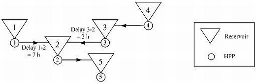
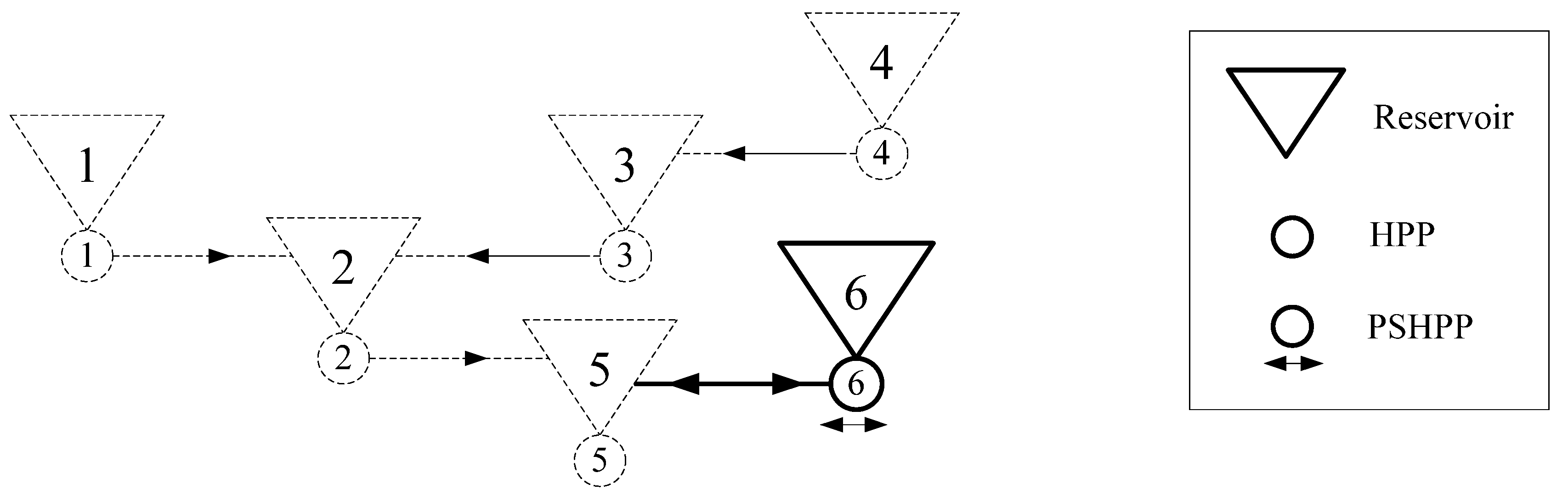
2.1. Model Overview
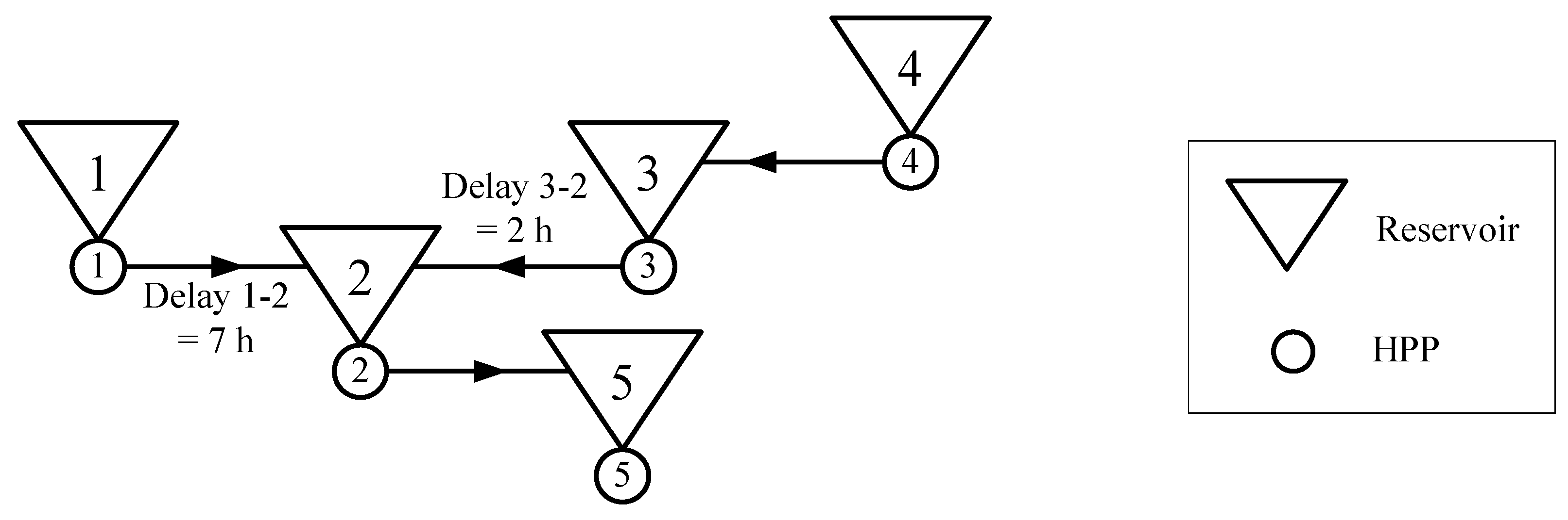
2.2. Water Balance
2.3. Input Data

| HPP | Reservoir | ||||||||||
|---|---|---|---|---|---|---|---|---|---|---|---|
| 1 | 2 | 3 | 4 | 6 | 1 | 2 | 3 | 4 | 6 | ||
| PMAX[MW] | 41.6 | 40.8 | 237 | 5 | 150 | XMIN(i) [e6 m3] | 300 | 1 | 0.6 | 200 | 4 |
| PMIN[MW] | 0 | 0 | 0 | 0 | 0 | XMAX(i) [e6 m3] | 800 | 2.6 | 1.6 | 560 | 13 |
| QMAX[m3/s] | 120 | 220 | 70 | 50 | 150 | X(i,0) [e6 m3] | 500 | 2 | 1.1 | 250 | 5 |
| BMIN[m3/s] | 0 | 0 | 0 | 0 | 0 | X(i,24) [e6 m3] | 500 | 2 | 1.1 | 250 | 5 |
| [MW] | [106m3] | [m3/s] | [MWs/m3] | ||||
|---|---|---|---|---|---|---|---|
| PMAX | 486 | XMAX | 4.4 | QMIN(5) | 75 | ∀ j ∈ J | |
| P01 | 115 | XMIN | 1.6 | QMAX(5,1) | 75 | ρj(1,5) | 1.8 |
| P02 | 125 | x(5,0) | 2 | QMAX(5,2) | 50 | ρj(2,5) | 2 |
| P03 | 135 | x(5,24) | 2 | QMAX(5,3) | 20 | ρj(3,5) | 5.8 |
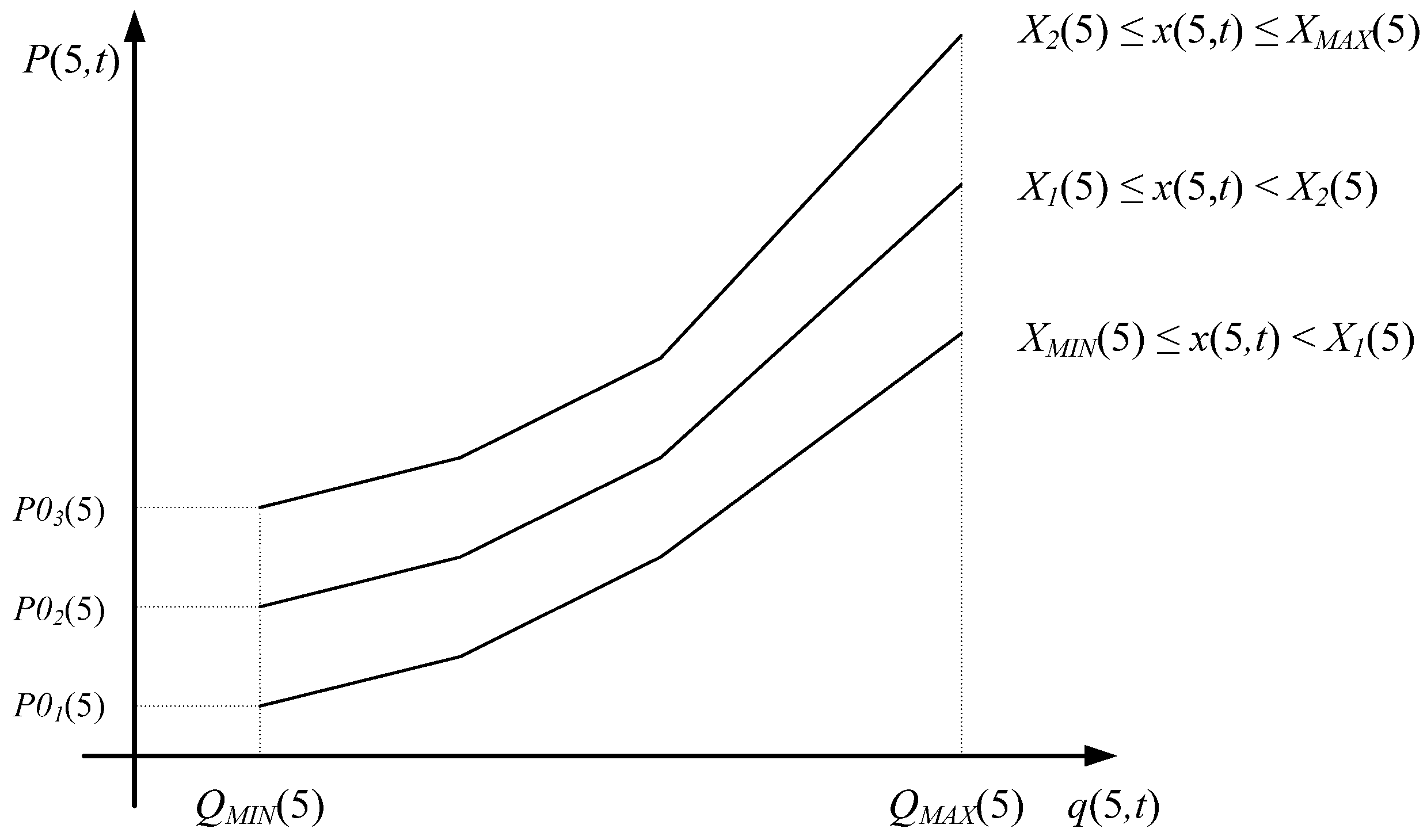
2.4. Formulation of Performance Curves
3. Problem Description
3.1. First Condition: Compensation for Using Water from the Reservoir 5
3.2. Second Condition: Preventing Spillage of Reservoir 5 by Forcing PC in Pump Regime
3.3. Third Condition: Preventing Spillage of Reservoir 5 by PC Refraining from Production
4. Model of PC-HC Symbiosis
4.1. First Condition: Compensation for Using Water from Reservoir 5
4.2. Second Condition: Preventing Spillage of Reservoir 5 by forcing PC in Pump Regime
4.3. Third Condition: Preventing Spillage of Reservoir 5 by PC Refraining from Production
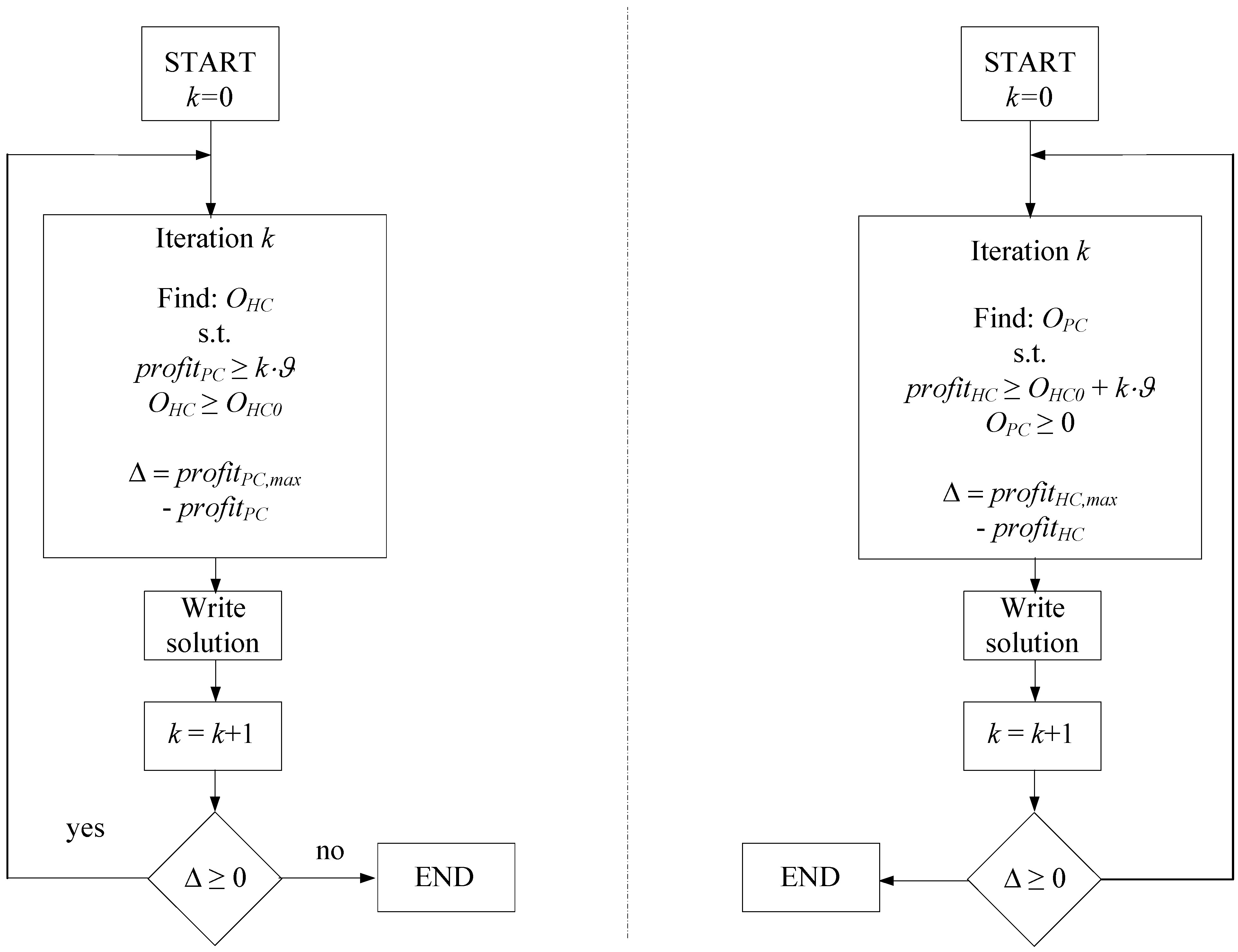
5. Search for an Optimal Solution


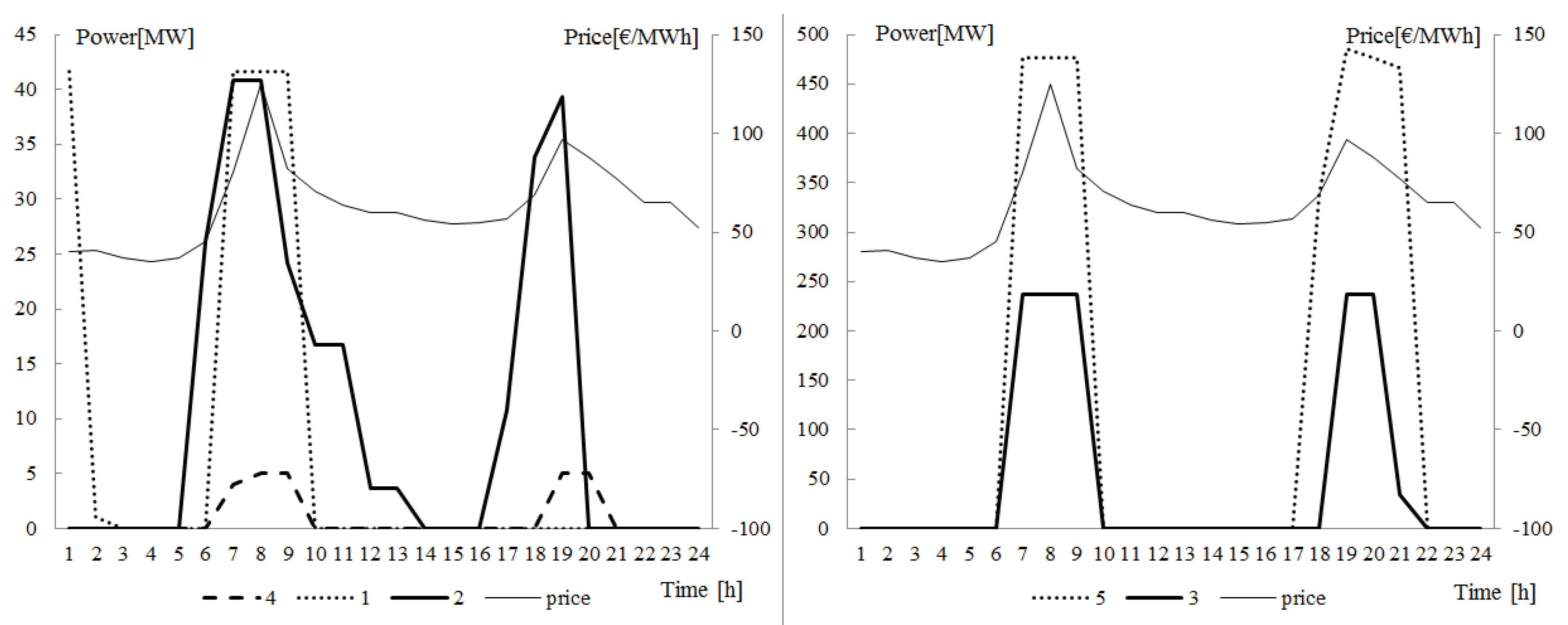
6. Case Study
| Reservoir | 1 | 2 | 3 | 4 | 5 | 6 |
|---|---|---|---|---|---|---|
| W(i,t) [m3/s] | 20 | 20 | 5 | 15 | 5 | 0 |
6.1. Base Model
6.1.1. Case A
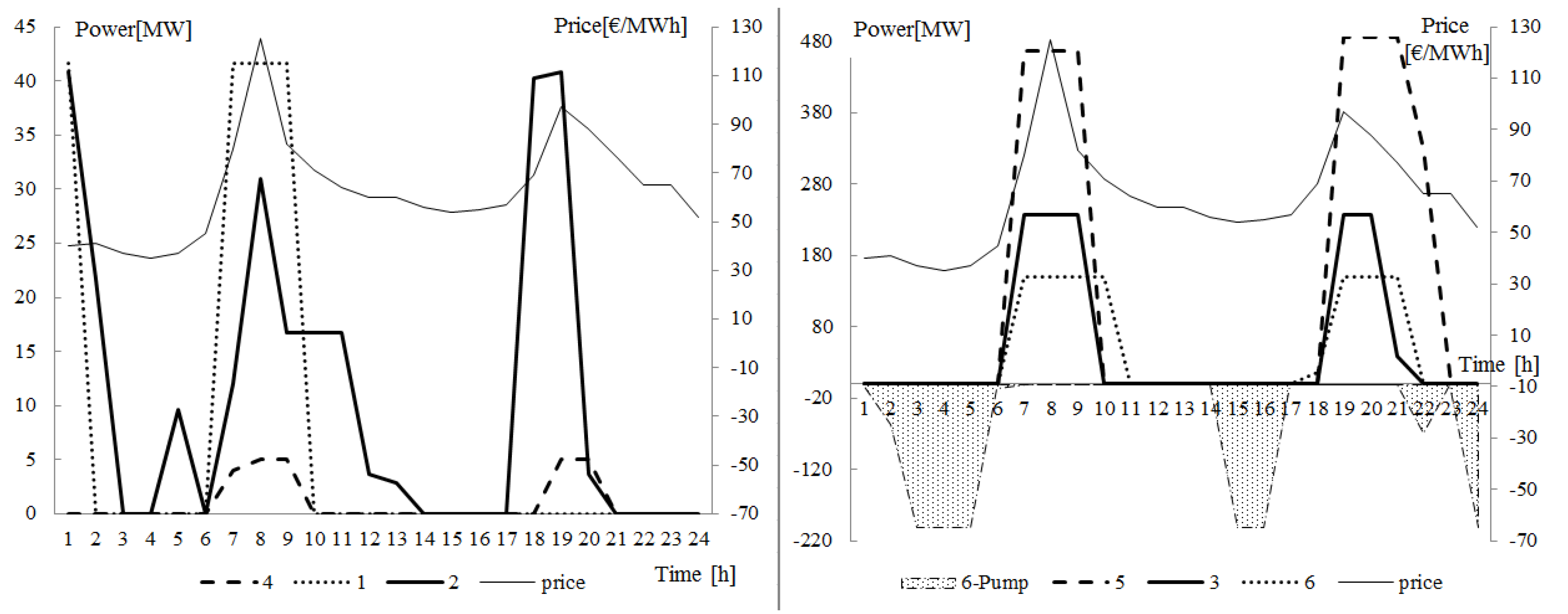
6.1.2. Case B
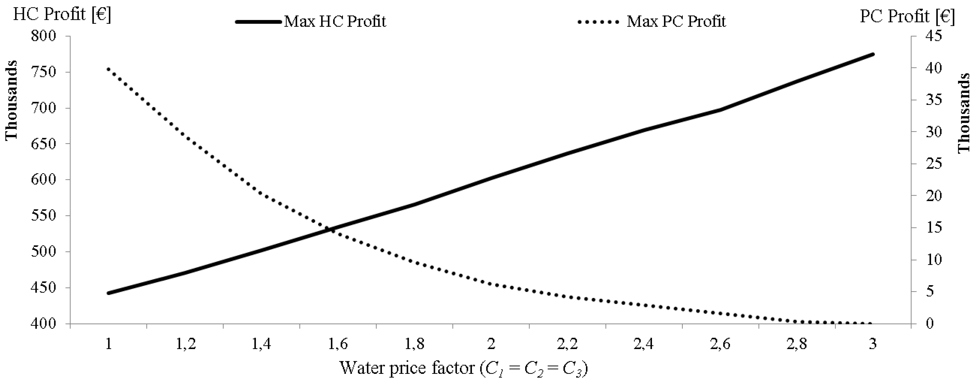
6.2. Water Price Factors Impacts on PC/HC Profit
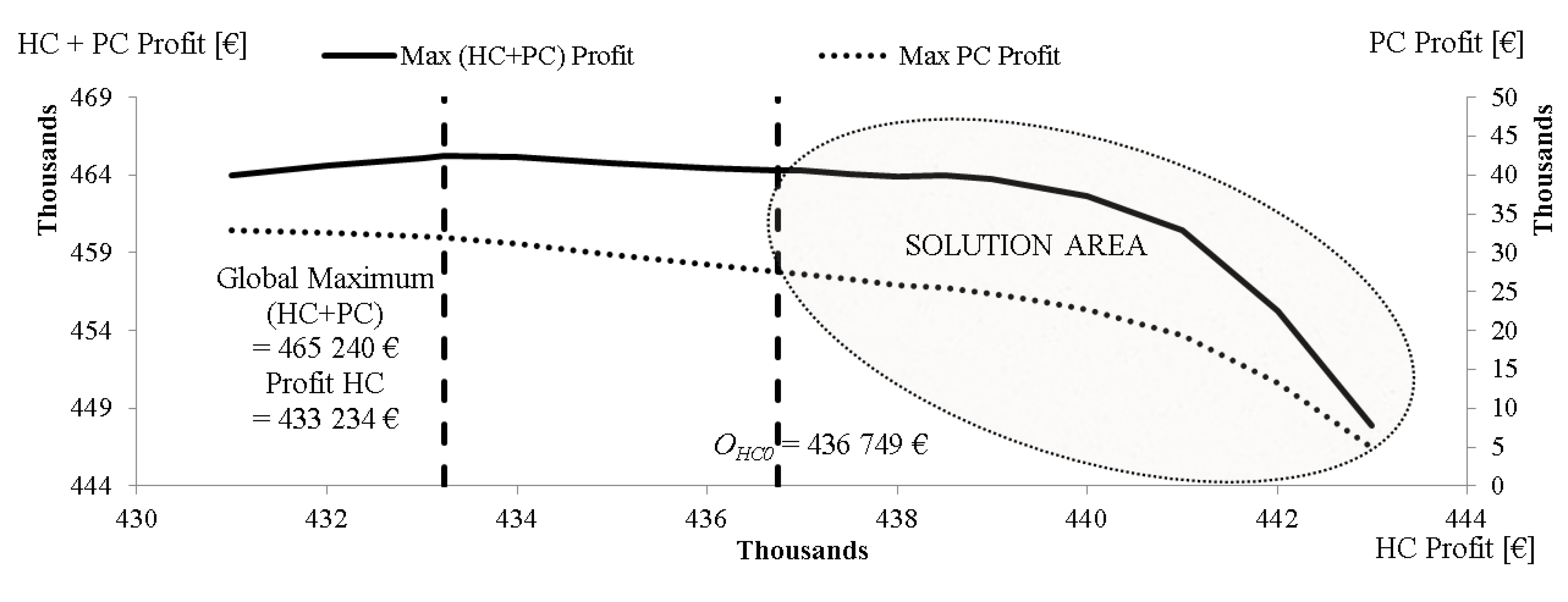
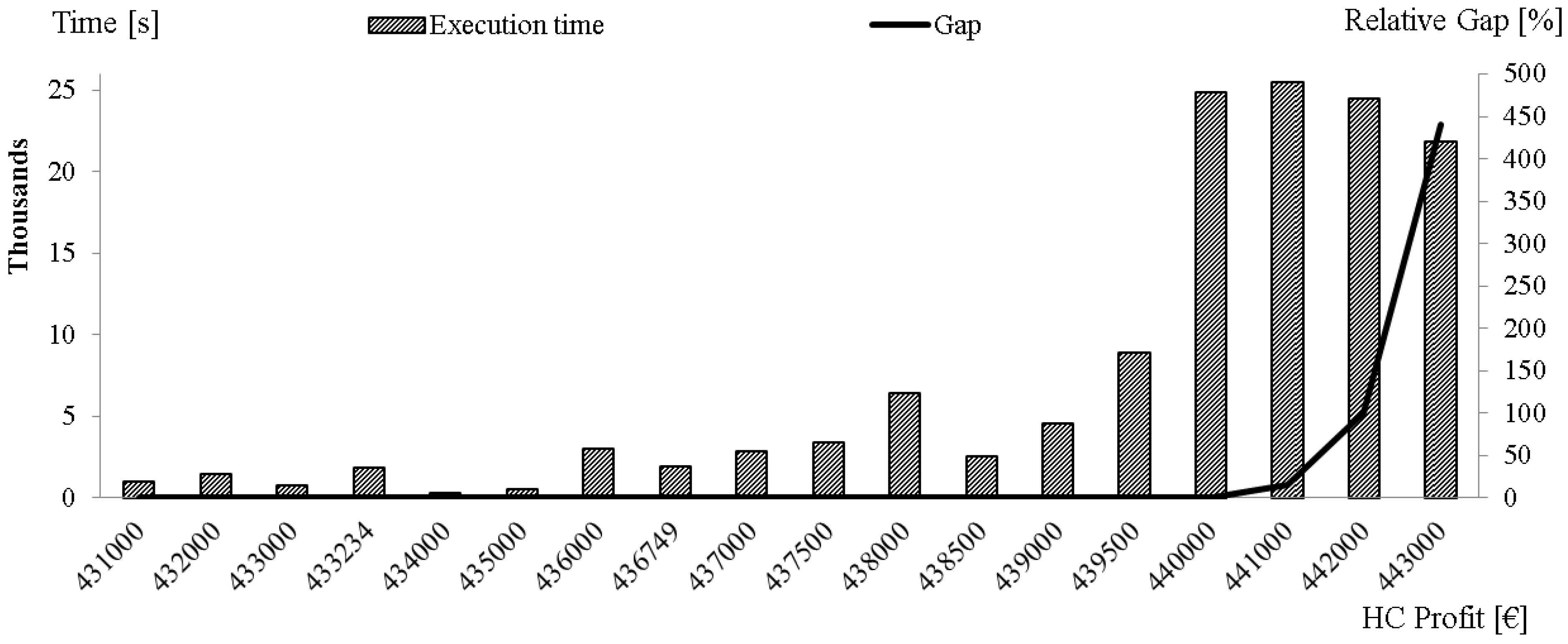
6.3. Set of Possible Solutions
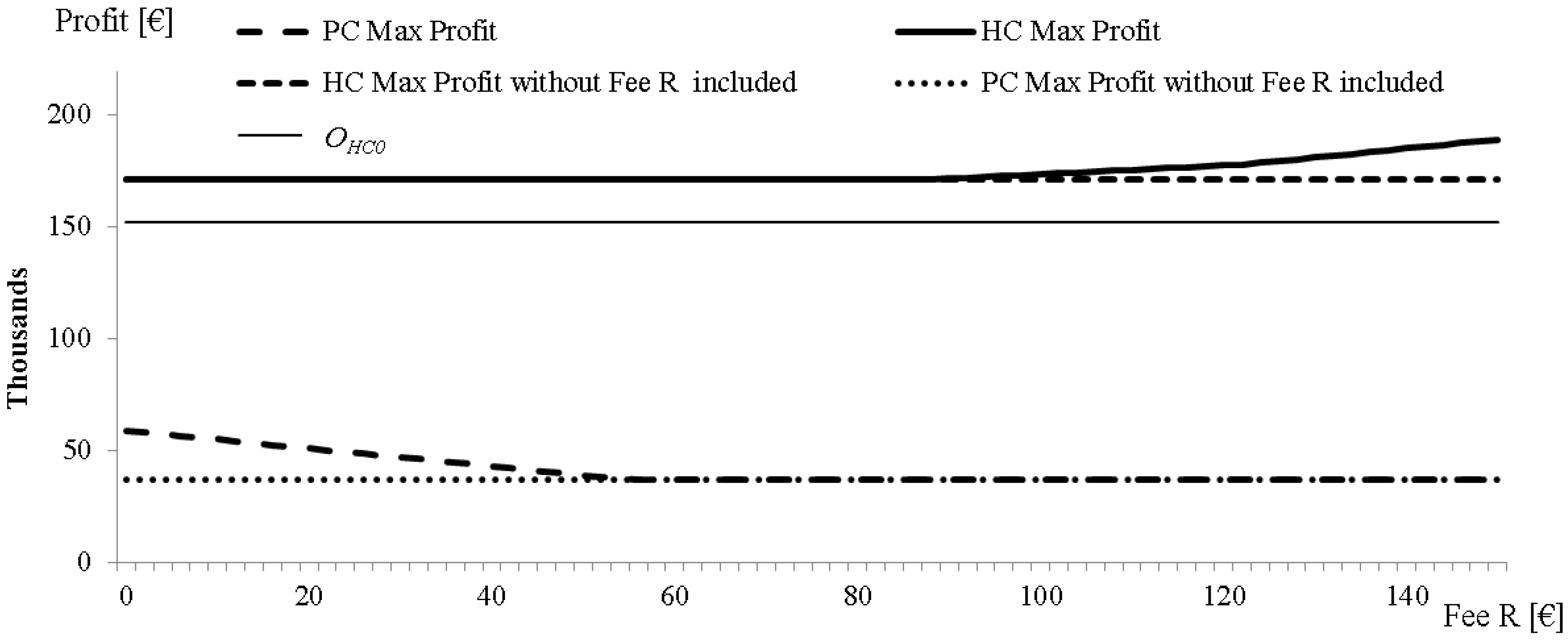
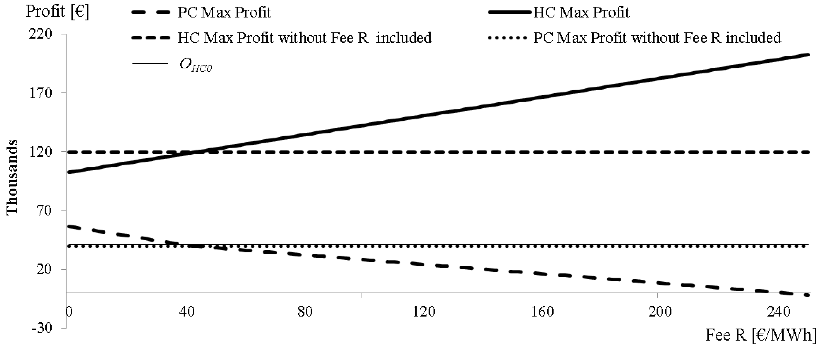
6.4. Fee R Impacts on PC/HC Profit

7. Conclusions
Nomenclature
| HPP | Hydro Power Plant. |
| PSHPP | Pumped Storage Hydropower Plant. |
| HC | Hydro Company. |
| PC | Pump Company that owns PSHPP 6. |
| T | Set of indices of the steps of the optimisation period, T = {1,2, …,24}, t T. |
| I | Set of indices of the reservoirs/plants, I= {1,2,3,4,5,6}, i I. |
| J | Set of indices of the perf. curves J= {1-high lvl., 2-middle lvl., 3-low lvl.}, j J. |
| Ui | Set of upstream reservoirs of plant i. |
| B | Set of indices of the blocks of the piecewise linearization of the unit performance curve B = {1,2,3}, b B. |
| M | Conversion factor equal to 3600 [m3s/m3h]. |
Water content of the reservoir i in time step t [m3]. | |
Average water content of the reservoir i in time step t [m3]. | |
Minimum content of the reservoir i [m3]. | |
First discrete level of the content of the reservoir i [m3]. | |
Second discrete level of the content of the reservoir i [m3]. | |
Maximum content of the reservoir i [m3]. | |
Initial water content of the reservoir i [m3]. | |
Final water content of the reservoir i [m3]. | |
Forecasted natural water inflow of the reservoir i in time step t [m3/s]. | |
Forecasted price of electricity in time step t [€/MWh]. | |
Price level that affects binary variable Fπ(t) in time step t [€/MWh]. | |
Water discharge of plant i in time step t [m3/s]. | |
Water discharge of block b of plant i in time step t [m3/s]. | |
Minimum water discharge of plant i [m3/s]. | |
Maximum water discharge of block b of plant i [m3/s]. | |
Maximum water discharge of plant i [m3/s]. | |
| BMIN(i) | Biological minimum of plant i [m3/s]. |
Maximum water intake of plant 6 (PSHPP) in pump regime [m3/s]. | |
Water intake of plant 6 (PSHPP) in pump regime in time step t [m3/s]. | |
Spillage of the reservoir i in time step t [m3/s]. | |
Time delay in water flow between reservoir j and i [h]. | |
| E | Large enough number for setting constraints. In this case 100,000. |
| ES | Large enough number for setting constraints. In this case 12 × 109. |
| Eπ | Large enough number for setting constraints. In this case 200. |
0/1 variable used for discretization of performance curves. | |
0/1 variable used for discretization of performance curves. | |
0/1 variable which is equal to 1 if plant i is on-line in time step t. | |
0/1 variable which is equal to 1 if plant 6 is in pump regime in time step t. | |
0/1 variable which is equal to 1 if water discharged by plant i has exceeded block b in time step t. | |
0/1 variable defined by Equation (19). | |
0/1 variable defined by Equation (20). | |
0/1 variable defined by Equation (21). | |
0/1 variable defined by Equation (22). | |
0/1 variable defined by Equation (23). | |
Power output of plant i in time step t [MW]. | |
Minimum power output of plant i for performance curve 1 (lower level of water content) [MW]. | |
Minimum power output of plant i for the performance curve 2 (intermediate level of water content) [MW]. | |
Minimum power output of plant i for the performance curve 3 (higher level of water content) [MW]. | |
Minimum power output of plant i [MW]. | |
Capacity of plant i [MW]. | |
Slope of the block b of the performance curve j of plant 5 [MWs/m3]. | |
Load of PSHPP 6 when working in pump regime in time step t [MW]. | |
Maximum load of PSHPP 6 [MW]. | |
Minimum load of PSHPP 6 [MW]. | |
| profitHC | Profit of HC during optimization time step [€]. |
| profitHC.max | Maximum possible HC profit or HC profit without constraints on the PC profit. |
| profitPC | Profit of PC during optimization time step [€]. |
| profitPC,max | Maximum possible PC profit or PC profit without constraints on the HC profit. |
| profit1,2,3,4,5 | Profit share of HC total profit gained by HPP 1 to 5 in Case A [€]. |
| profitPSHPP | Profit share of HC total profit gained by PSHPP 6 in Case A [€]. |
Arbitrarily chosen step in the optimization procedure (1, 10, 100, etc.). |
References
- Zhang, D.; Luh, P.B.; Zhang, Y. A bundle method for hydrothermal scheduling. IEEE Trans. Power Syst. 1999, 14, 1355–1361. [Google Scholar] [CrossRef]
- George, A.; Reddy, C.; Sivaramakrishnan, A.Y. Multi-objective, short-term hydro thermal scheduling based on two novel search techniques. Int. J. Eng. Sci. Technol. 2010, 2, 7021–7034. [Google Scholar]
- Dhillon, Jarnail S.; Dhillon, J.S.; Kothari, D.P. Multi-objective short-term hydrothermal scheduling based on heuristic search technique. Asian J. Inf. Technol. 2007, 6, 447–454. [Google Scholar]
- Zhang, J.L.; Ponnambalam, K. Hydro energy management optimization in a deregulated electricity market. Optim. Eng. 2006, 7, 47–61. [Google Scholar] [CrossRef]
- Horsley, A.; Wrobel, A.G. Profit-maximizing operation and valuation of hydroelectric plant: A new solution to the Koopmans problem. J. Econ. Dyn. Control 2007, 31, 938–970. [Google Scholar] [CrossRef]
- Garcia-Gonzalez, J.; Parrilla, E.; Mateo, A. Risk-averse profit-based optimal scheduling of a hydro-chain in the day-ahead electricity market. Eur. J. Oper. Res. 2007, 181, 1354–1369. [Google Scholar] [CrossRef]
- Garcia-Gonzalez, J.; Parrilla, E.; Mateo, A.; Moraga, R. Building Optimal Generation Bids of a Hydro Chain in the Day-Ahead Electricity Market under Price Uncertainty. In Proceedings of the 2006 International Conference on Probabilistic Methods Applied to Power Systems (PMAPS 2006), Stockholm, Sweden, 11–15 June 2006; pp. 1–7.
- Fleten, S.E.; Kristoffersen, T.K. Stochastic programming for optimizing bidding strategies of a Nordic hydropower producer. Eur. J. Oper. Res. 2007, 181, 916–928. [Google Scholar] [CrossRef]
- Wangesteen, I. Power System Economics: The Nordic Electricity Market; Tapir Academic Press: Trondheim, Norway, 2007. [Google Scholar]
- Luiz da Silva, E.; Finardi, E.C. Parallel processing applied to the planning of hydrothermal systems. IEEE Trans. Parallel Distrib. Syst. 2003, 14, 721–729. [Google Scholar] [CrossRef]
- Mariano, S.J.P.; Catalao, J.P.S.; Mendes, V.M.F.; Ferreira, L.A.F.M. Profit-Based Short-Term Hydro Scheduling Considering Head-Dependent Power Generation. In Proceedings of the 2007 IEEE Power Tech, Lausanne, Switzerland, 1–5 July 2007; pp. 1362–1367.
- Conejo, A.J.; Arroyo, J.M.; Contreras, J.; Villamor, F.A. Self-scheduling of a hydro producer in a pool-based electricity market. IEEE Trans. Power Syst. 2002, 17, 1265–1272. [Google Scholar] [CrossRef]
- Ponrajah, R.A.; Galiana, F.D. Systems to Optimise Conversion Efficiencies at Ontario Hydro’s Hydroelectric Plants. In Proceedings of the 1997 International Conference on Power Industry Computer Applications, Columbus, OH, USA, 11–16 May 1997; pp. 245–251.
- Kazempour, S.J.; Hosseinpour, M.; Moghaddam, M.P. Self-Scheduling of a Joint Hydro and Pumped-Storage Plants in Energy, Spinning Reserve and Regulation Markets. In Proceedings of the 2009 IEEE Power & Energy Society General Meeting (PES '09), Calgary, Canada, 26–30 July 2009; pp. 1–8.
- Gao, H.M.; Wang, C. Detailed Pumped Storage Station Model for Power System Analysis. In Proceedings of the 2006 IEEE Power Engineering Society General Meeting, Montreal, Canada, 18–22 June 2006.
- Genoese, F.; Genoese, M.; Wietschel, M. Occurrence of Negative Prices on the German Spot Market for Electricity and Their Influence on Balancing Power Markets. In Proceedings of the 2010 International Conference on the European Energy Market (EEM), Madrid, Spain, 23–25 June 2010; pp. 1–6.
- Mandić, N. Najsuvremenija reverzibilna hidroelektrana u Europi. EGE 2011, 2, 55–58. [Google Scholar]
- Goić, R.; Lovrić, M. Mogućnosti Efikasnijeg Operativnog Planiranja Rada i Vođenja HES—A Rijeke Cetine; IV Savjetovanje HK Cigre: Cavtat, Croatia, 17–21 October 1999; pp. 67–75. [Google Scholar]
- Rosenthal, R. GAMS-A User’s Guide; GAMS Development Corporation: Washington, DC, USA, 2012. Available online: http://www.gams.com/dd/docs/bigdocs/GAMSUsersGuide.pdf (accessed on 16 August 2012).
© 2012 by the authors; licensee MDPI, Basel, Switzerland. This article is an open access article distributed under the terms and conditions of the Creative Commons Attribution license (http://creativecommons.org/licenses/by/3.0/).
Share and Cite
Rajšl, I.; Ilak, P.; Delimar, M.; Krajcar, S. Dispatch Method for Independently Owned Hydropower Plants in the Same River Flow. Energies 2012, 5, 3674-3690. https://doi.org/10.3390/en5093674
Rajšl I, Ilak P, Delimar M, Krajcar S. Dispatch Method for Independently Owned Hydropower Plants in the Same River Flow. Energies. 2012; 5(9):3674-3690. https://doi.org/10.3390/en5093674
Chicago/Turabian StyleRajšl, Ivan, Perica Ilak, Marko Delimar, and Slavko Krajcar. 2012. "Dispatch Method for Independently Owned Hydropower Plants in the Same River Flow" Energies 5, no. 9: 3674-3690. https://doi.org/10.3390/en5093674
APA StyleRajšl, I., Ilak, P., Delimar, M., & Krajcar, S. (2012). Dispatch Method for Independently Owned Hydropower Plants in the Same River Flow. Energies, 5(9), 3674-3690. https://doi.org/10.3390/en5093674