A spin-down test is performed by accelerating the motor to its peak rotational speed, disconnecting the power supply and load, and allowing the rotor to spin down due to internal losses. This test was performed several times under varying levels of vacuum in order to calculate the losses associated with the total amount of energy stored in the flywheel. The open-circuit line-to-line voltage induced in the windings on the low power side was recorded continuously during the tests. The frequency of this voltage was then used to calculate the instantaneous mechanical speed, which in turn was used to calculate the total amount of kinetic energy,
EK, stored in the flywheel, using the formula:
where
I is the moment of inertia of the flywheel and
ωm is the angular velocity of the rotor. As a consequence, the total instantaneous power loss from mechanical friction, eddy currents and drag could be calculated through derivation of the kinetic energy with respect to time, see
Figure 4.
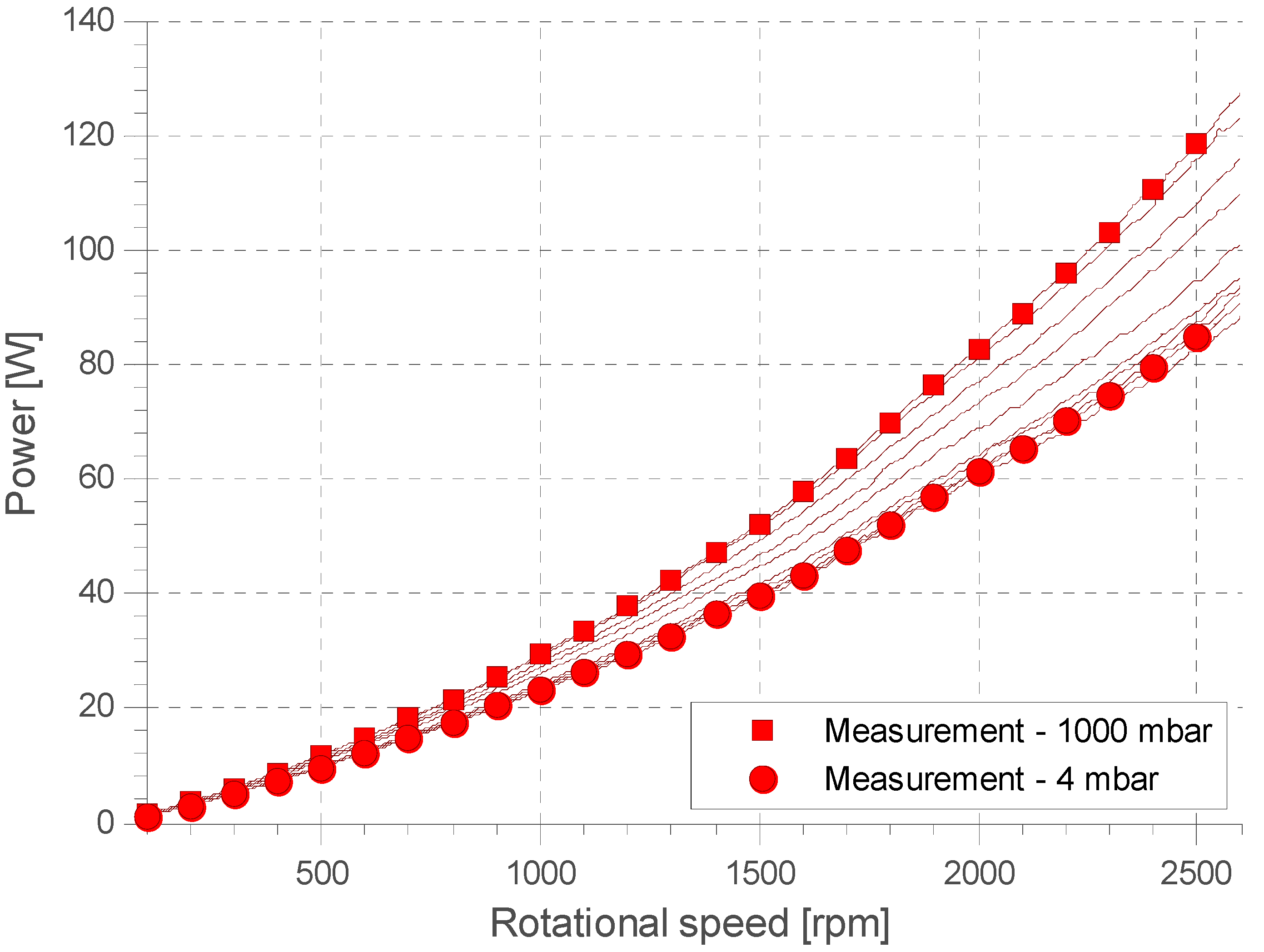
Figure 4.
Measurement of power loss during spin-down test. The instantaneous power loss was estimated by numerical derivation of the stored kinetic energy with time. The higher losses correspond to higher pressures. The upper limit correspond to a pressure of 1000 mbar (atmospheric pressure), and the lower limit to 4 mbar.
The measurement comprised the sum of drag, eddy-current loss and bearing loss. In order to verify the theoretical models, it was necessary quantify the impact of each loss mechanism individually. The first step to this end was to extract the losses due the drag.
3.1.1. Air Friction
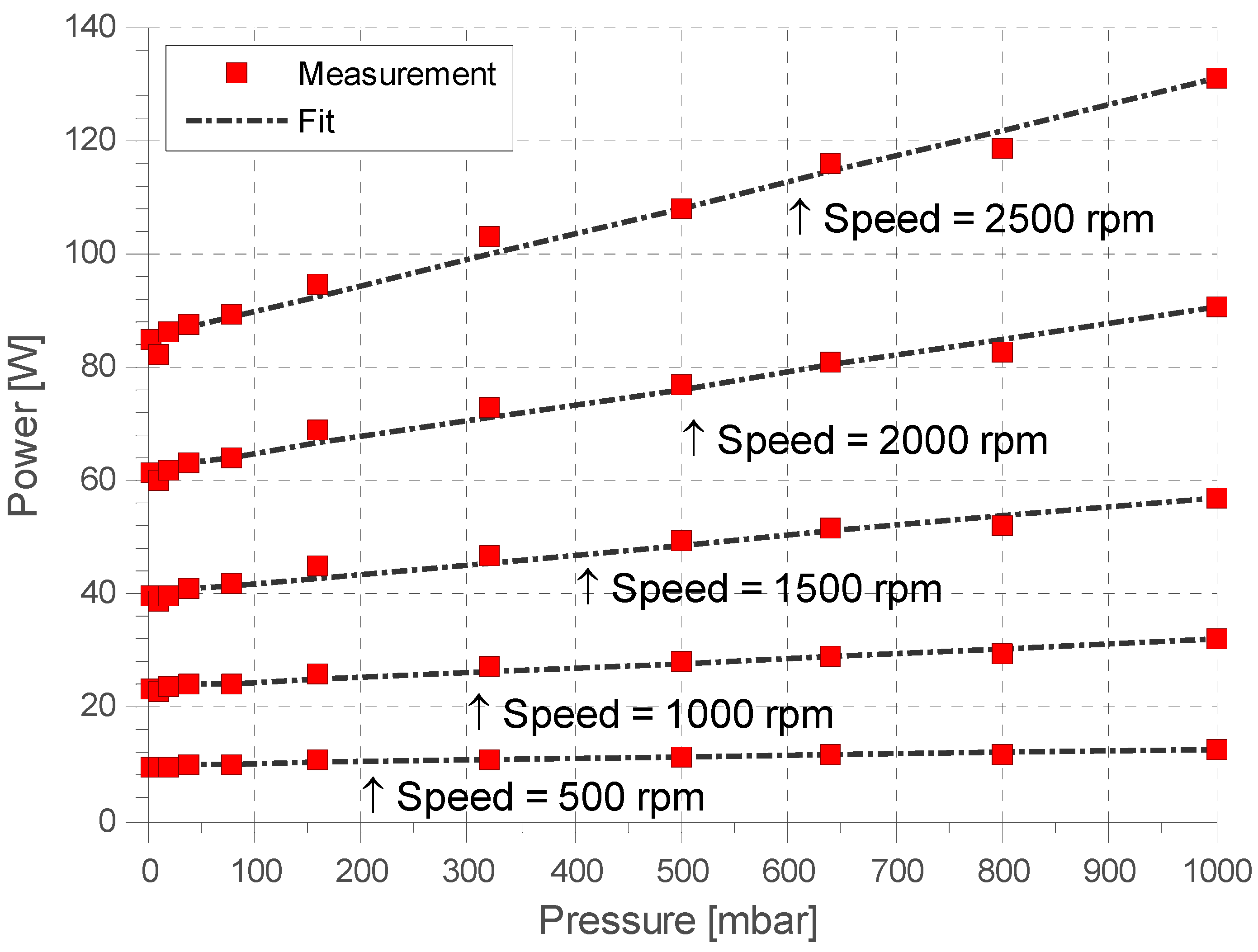
By varying the level of vacuum in the chamber, and measuring the power loss over rotational speed, the effect of drag was quantified. The minimum pressure reached was 4 mbar. By extrapolating the results down to 0 mbar, the total loss due to air friction was estimated, see
Figure 5. The drag losses were found to scale linearly with the density of the air, as expected from Equation (12).
Figure 5.
Air friction loss over pressure. Note the linear dependence of power loss on air density.
Figure 5.
Air friction loss over pressure. Note the linear dependence of power loss on air density.
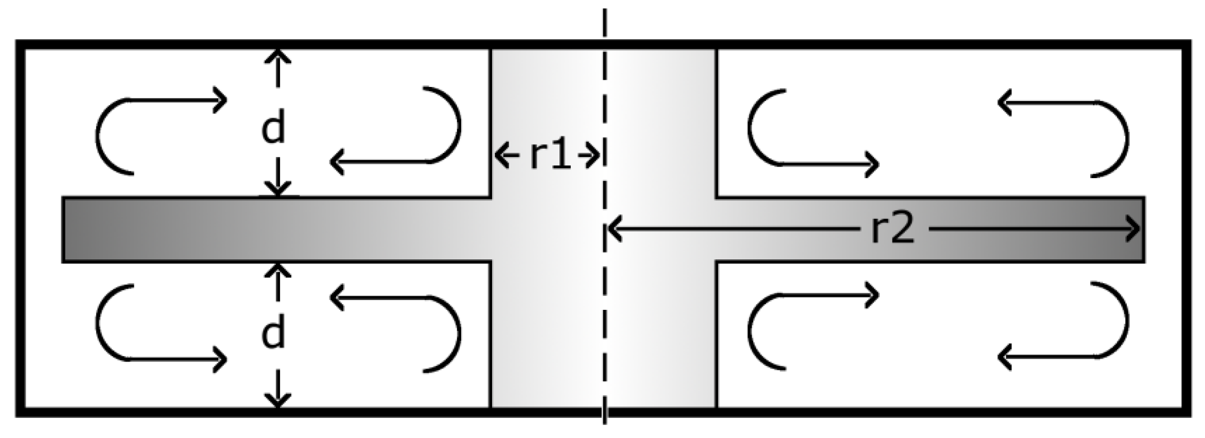
The geometry of the electric machine can be seen in
Figure 6. It was assumed that no gas flows axially between the different sections. The machine could under this assumption be modelled as two separate discs, contained in cylindrical enclosures.
According to Equations (11) and (12), the power loss due to air friction became:
where
Cf1 is the friction coefficient for the disc with axial clearance
d1 and
Cf2 the friction coefficient for the disc with axial clearance
d2. The difference in axial clearance caused a difference in friction coefficient for the same rotational speed even thought the surface roughness was assumed to be the equal.
Further, an estimation of the different flow regimes occurring in the motor was required in order to estimate the two friction coefficients. The parameters used in the calculation of the power loss for the two discs can be found in
Table 6.
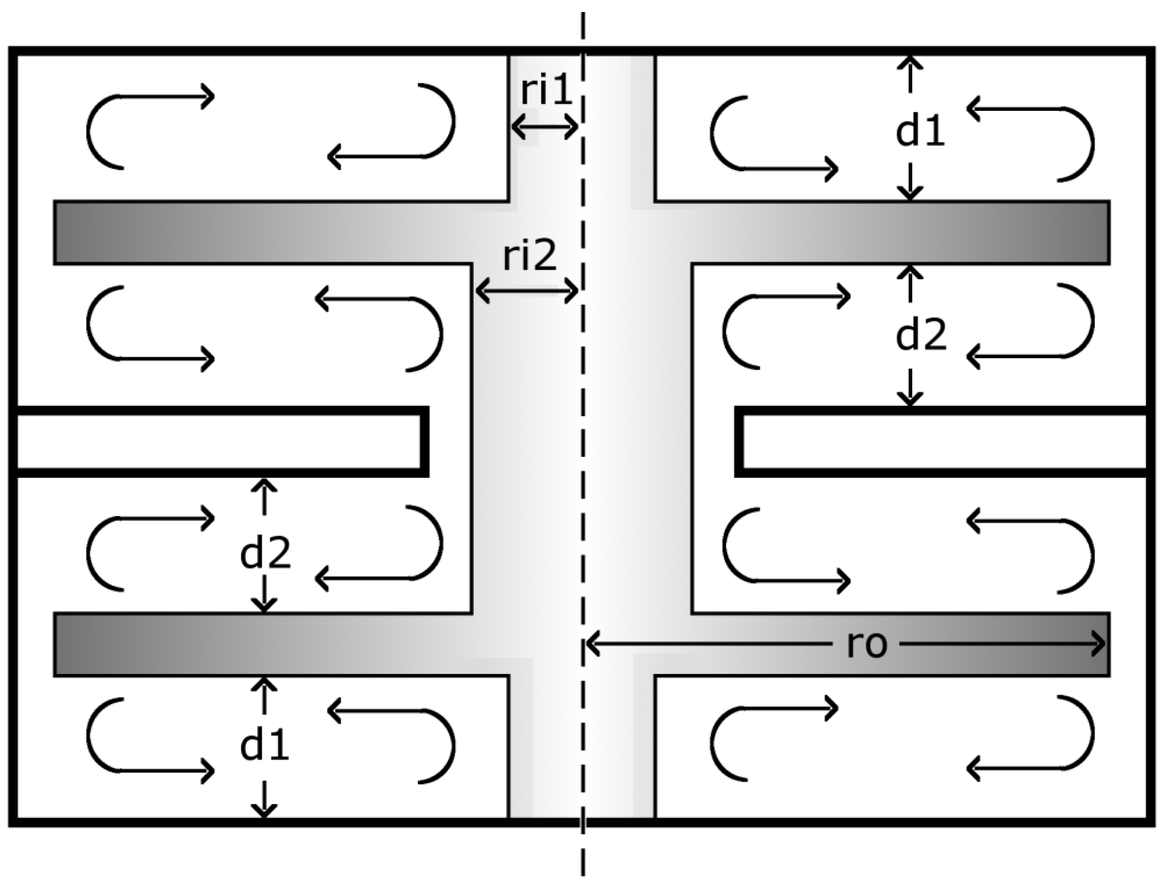
Figure 6.
The power loss due to air friction can be estimated by approximating the shape of the rotor as two discs enclosed in cylindrical boxes. The arrows illustrate the radial mass transport associated with the turbulent flows found in regimes II and IV.
Figure 6.
The power loss due to air friction can be estimated by approximating the shape of the rotor as two discs enclosed in cylindrical boxes. The arrows illustrate the radial mass transport associated with the turbulent flows found in regimes II and IV.
Table 6.
Parameters used in the calculation of power loss due to air friction.
Table 6.
Parameters used in the calculation of power loss due to air friction.
| Symbol | Parameter | Unit | Value |
|---|
| ρa | Density of air | kg/m3 | 1.2 |
| μ | Dynamic viscosity | Ns/m2 | 19.6 × 10⁻⁶ |
| ri1 | Inner radius of rotor | m | 15 × 10−3 |
| ri2 | Inner radius of rotor | m | 47.5 × 10⁻³ |
| ro | Outer radius of rotor | m | 165 × 10−3 |
| d1 | Axial gap for rotor 1 | m | 10 × 10−3 |
| d2 | Axial gap for rotor 2 | m | 20 × 10−3 |
These parameters, together with those in
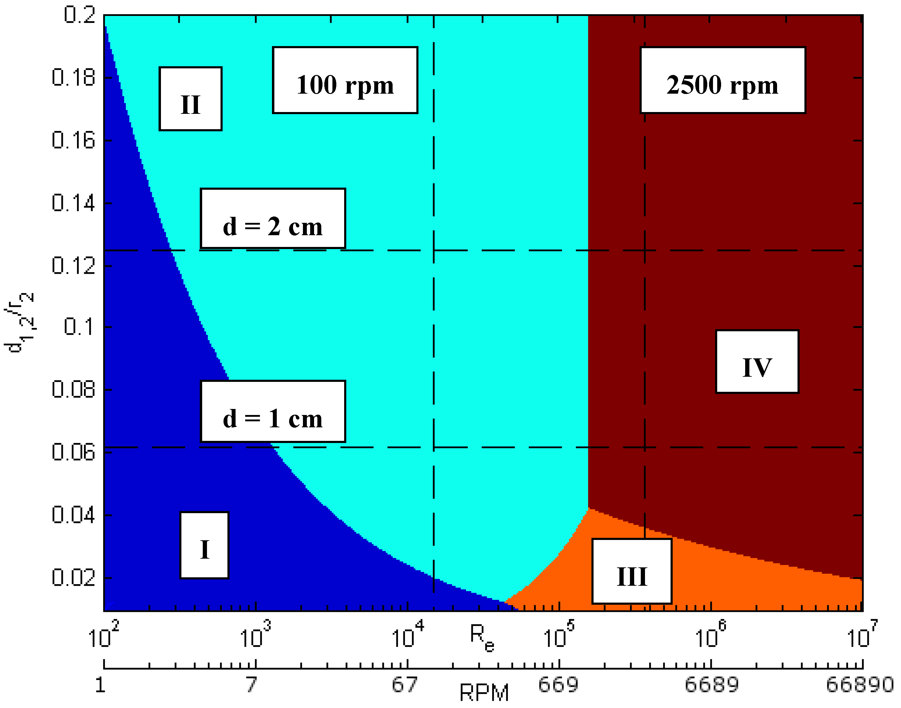
Table 5, were used to generate a theoretical plot of the different flow regimes occurring in the motor as function of Reynolds number and spacing ratio, see
Figure 7. The horizontal lines mark the impact of the axial gap distance for the two discs. The vertical lines mark the actual region of operation.
The plot shows that the discs were operating in regime I, corresponding to a situation with laminar flow and merged boundary layers, for very low speeds. However, both discs had already transitioned into regime II at 10 rpm, meaning predominantly laminar flow but with separated boundary layers. Approximately around 1000 rpm, the discs continued into regime IV, a region with turbulent flow and separated boundary layers. The system never entered into region III, corresponding to turbulent flow and merged boundary layers.
Figure 7.
Theoretical flow regimes as function of Reynolds number (rotational speed) for the constructed geometry. The transition from region II to region IV was found to take place at a rotational velocity of around 905 rpm for spacing ratios higher than 0.05.
Figure 7.
Theoretical flow regimes as function of Reynolds number (rotational speed) for the constructed geometry. The transition from region II to region IV was found to take place at a rotational velocity of around 905 rpm for spacing ratios higher than 0.05.
From this it could be concluded that regime II and IV were responsible for the majority of the drag losses. The corresponding friction coefficients were:
The transition from regime II to regime IV occurred when the friction coefficients of the two regimes were equal, leading to a Reynolds number of:
This transition Reynolds number was in this case independent on the spacing ratio, and so corresponded to a rotational velocity of 905 rpm for both discs.
The total power loss due to air friction in the system could now be calculated by:
with:
However, to fully quantify the power loss due to air friction, the surface roughness factor,
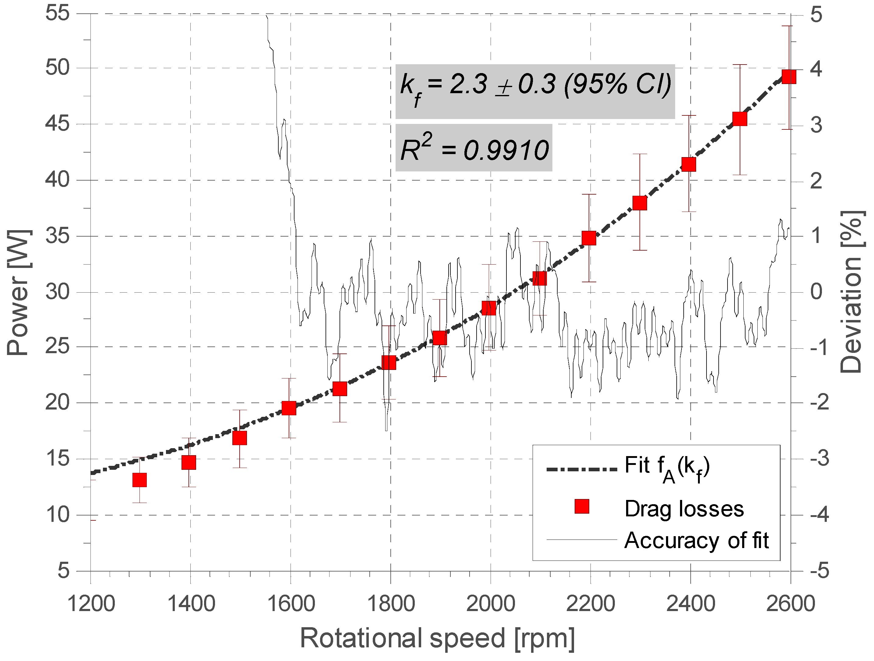
kf, needed to be determined. It was evaluated by comparing the theoretical power loss with the measured one in regime IV (over 1200 rpm), see
Figure 8. In this evaluation, the theoretical values were forced to coincide with the measured values at a rotational speed of 2600 RPM.
Figure 8.
Measured power loss due to air friction at 1 bar. A roughness factor of 2.3 ± 0.3 was required in order to reproduce the measured values.
Figure 8.
Measured power loss due to air friction at 1 bar. A roughness factor of 2.3 ± 0.3 was required in order to reproduce the measured values.
The fit of measured power loss together with the analytical analysis revealed that the surface roughness factor amounted to 2.3 ± 0.3. This was found to correspond well with previously reported values, see
Table 4.
After having fully quantified the losses due to drag, the next step of the analysis was to separate the remaining losses from each other. No direct measurement of these individual loss components was possible. Instead, the theoretical background for each loss mechanism was used to extract the components of the loss-curve belonging to signals with different dependencies on rotational speed.
3.1.2. Detailed Analysis of Bearing Loss
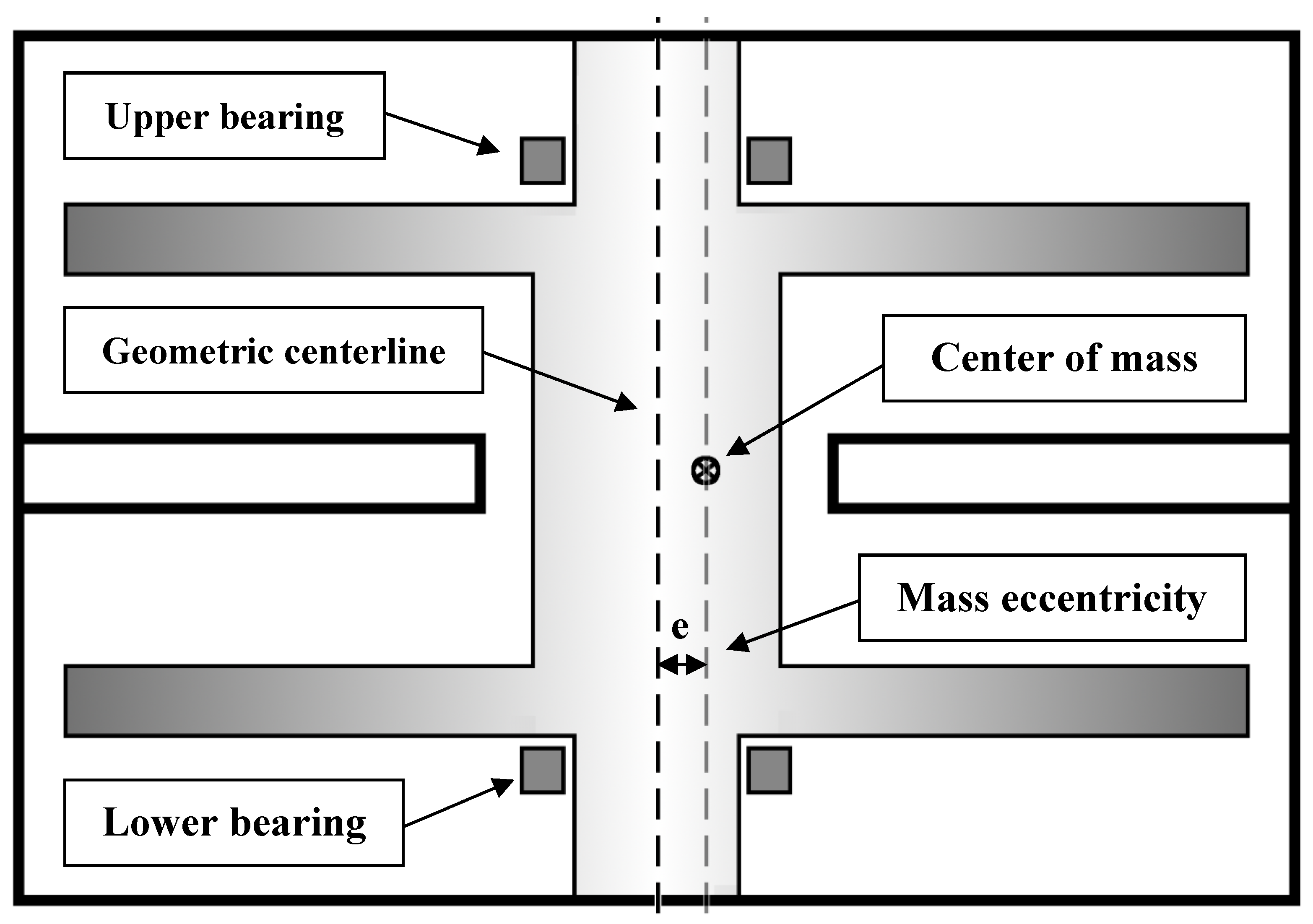
The geometry of the electric machine and position of the ball bearings can be seen in
Figure 9. The machine was constructed in such a way that the bottom ball bearing supported the complete axial load of the rotor. It was further assumed that the radial load was divided equal between the upper and lower bearings.
The bearings used were of the SKF 6205-2RSH type, sealed for life and lubricated with a mineral oil-based grease—LGMT 2. Thermal measurements in the bearing region showed that the temperature in the region of the bearings was approximately 60 °C ± 10 °C, corresponding to a range of kinematic viscosity from 60.5 mm
2/s to 93.5 mm
2/s, with an average of 77 mm
2/s. The required properties of these bearings can be found in
Table 7.
Figure 9.
Geometry of the electric machine and position of the ball bearings.
Figure 9.
Geometry of the electric machine and position of the ball bearings.
Table 7.
Parameters used in the calculation of power loss due to mechanical bearings. All parameters for a given bearing geometry and lubrication can be found in [
19] and [
26].
Table 7.
Parameters used in the calculation of power loss due to mechanical bearings. All parameters for a given bearing geometry and lubrication can be found in [19] and [26].
| Symbol | Parameter | Unit | Value |
|---|
| ν | Kinematic viscosity of grease | mm2/s | 60.5–93.5 |
| Fa | Axial force on lower bearing | N | 191 |
| C0 | Basic static load rating | N | 7800 |
| μsl | Sliding friction coefficient | n/a | 0.05 |
| dm | Average bearing diameter | mm | 38.5 |
| R1, R2 | Geometry constants, rolling | n/a | 3.9 × 10⁻⁷, 1.7 |
| S1, S2 | Geometry constants, sliding | n/a | 3.23 × 10⁻³, 36.5 |
| KS1, KS2, β | Geometry constants, seal | n/a | 0.028, 2, 2.25 |
| ds | Seal counter-face diameter | mm | 31.8 |
| τseal | Measured seal friction | Nmm | 72 |
Direct measurements of the frictional torque from the seals of the bearings were performed. The measurements indicated that each bearing was exposed to an approximate torque of 72 Nmm. This value deviated significantly from the nominal value of 82.2 Nmm, calculated from geometry according to
Table 3. The measured value was used in the further analysis.
The only remaining unknown factor impacting the losses in the bearing was the rotor imbalance, er. The imbalance of the rotor was therefore left as a free parameter, to be estimated from the measurements.
3.1.4. Estimating the Fit-parameters
After removing the extrapolated drag loss at zero pressure from the measurements, the sum of mechanical and eddy current losses remained from the measurements. Of these remaining losses the electrical losses increased as the square of the rotational velocity, as shown in
Section 2.3. The mechanical losses had a more complex dependency, with a strong linear component as well as several nonlinear ones.
By using the theoretical framework describing the rotational dependence of the losses, the two unknown parameters
er and
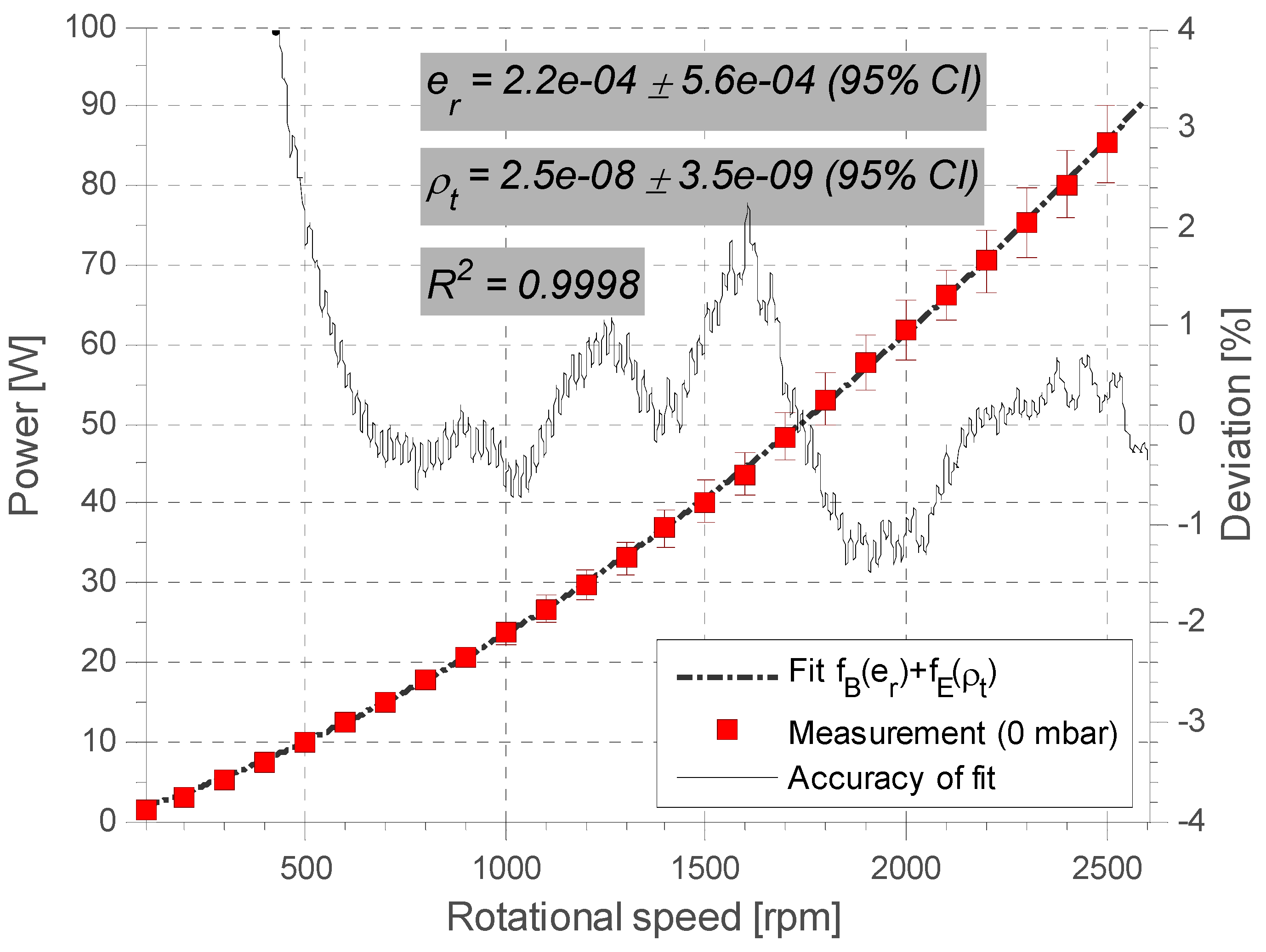
ρt could be estimated. This was achieved by minimizing the difference between the measured and simulated total loss, using the method of least squares. A plot of the correspondence between total measured loss and the sum of the simulated losses according to the above criteria can be found in
Figure 10.
The parameters evaluated to
er = 2.2 × 10
−4 ± 5.6 × 10
−4 and
ρt = 2.5 × 10
−8 ± 3.5 × 10
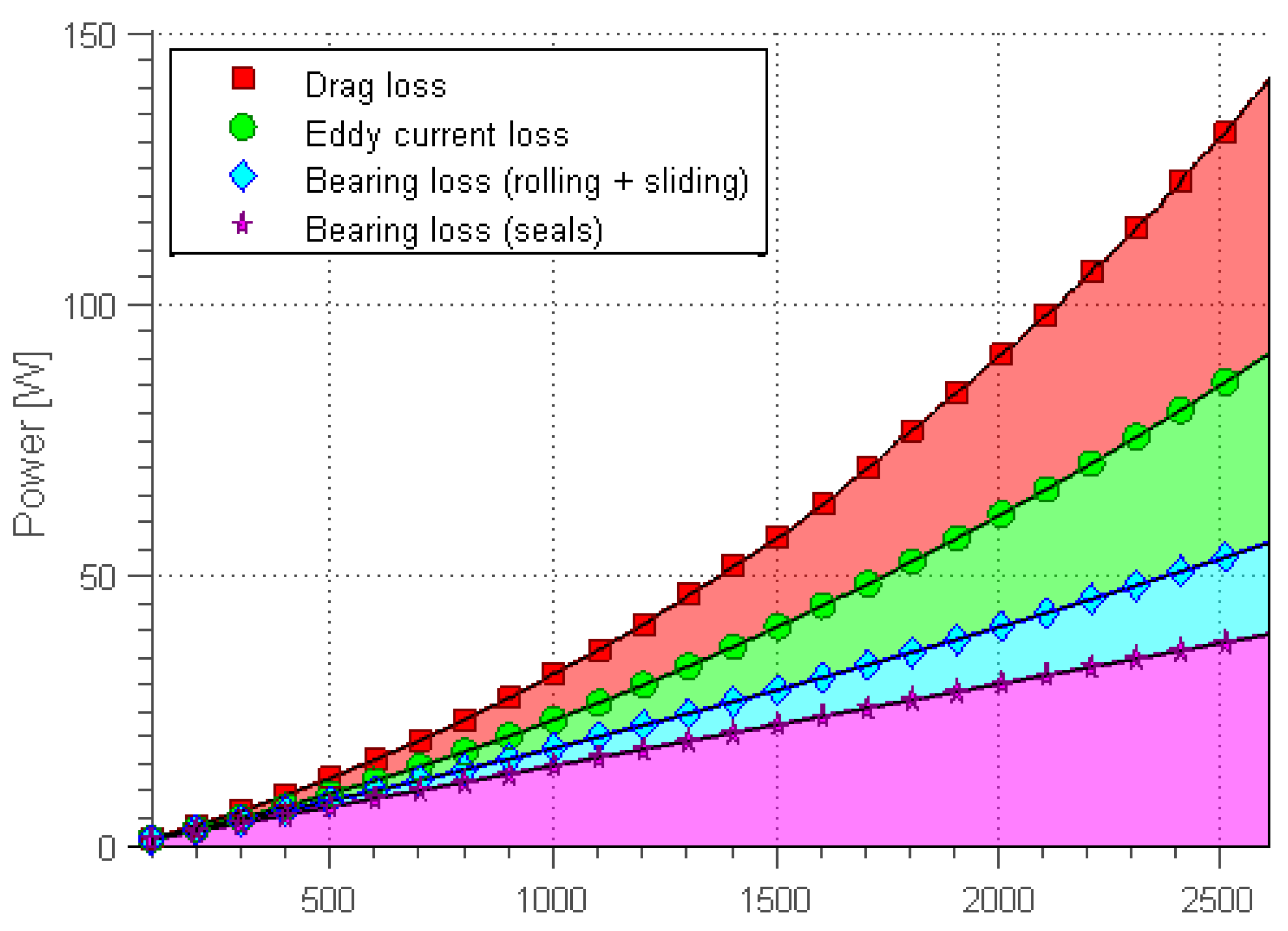
−9. After obtaining these estimations on imbalance and resistivity, the complete decomposition of the measured losses in their individual components could be plotted,
Figure 11.
Figure 10.
Fit of calculated to measured total power loss using the least squares method, by varying two parameters(er and ρt) corresponding to mechanical imbalance and perpendicular resistivity of the conductors.
Figure 10.
Fit of calculated to measured total power loss using the least squares method, by varying two parameters(er and ρt) corresponding to mechanical imbalance and perpendicular resistivity of the conductors.
Figure 11.
Decomposition of power loss using the dependence on rotational speed.
Figure 11.
Decomposition of power loss using the dependence on rotational speed.

