1. Introduction
The transportation sector is a major consumer of fossil fuel, thus eliminating or reducing pollution from transportation sources is a majority policy objective. Many researchers have focused on the chemical reactions of producing electrical energy from hydrogen. Proton Exchange Membrane (PEM) fuel cells (FCs) have been the most attractive energy conversion technology because of their high efficiency, low operating temperature (50 °C–100 °C), zero emissions, quick start-up and high environmental friendliness. A basic schematic of a PEM fuel cell is shown in
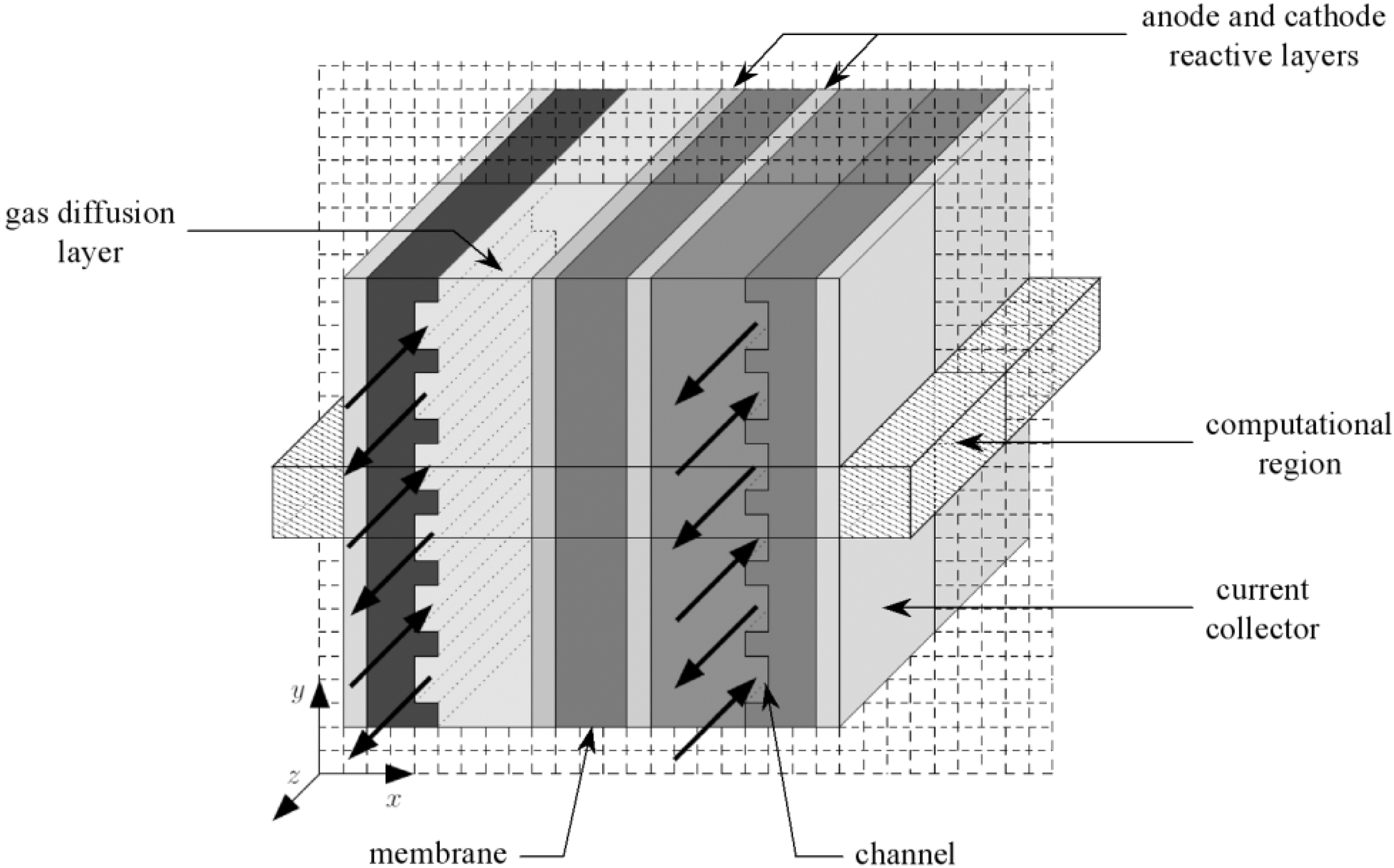
Figure 1. On the anode side, hydrogen flows into the gas channels and diffuses through the gas diffusion layer. Then hydrogen gets to the catalyst layer where it dissociates into electrons and protons through a chemical reaction. The electrons are forced to the cathode side through an external circuit, because the membrane is electrically insulating while the protons are conducted across the membrane towards the cathode. On the cathode side, oxygen also arrives at the catalyst layer through the gas diffusion layer. Subsequently, oxygen molecules react with the electrons which have travelled through the external circuit and protons combine to form molecules of water.
Figure 1.
Internal structure of a single fuel cell.
Figure 1.
Internal structure of a single fuel cell.
The heart of fuel cell is a device involving multi-physics coupling phenomena: mass transport (in the electrodes and electrolyte), charge transport (in the electrolyte), and electrochemical kinetics (at reactive sites). To these phenomena, are added problems of thermal and distribution of reactive gases. Many mathematical models can locally describe these phenomena, by means of partial differential equations involving space and time [
1,
2,
3,
4,
5,
6,
7,
8]. These models are accurate, but most of time unusable for a systems approach. That is the reason why some electrical circuit models have been developed. However in last few years, researchers have realized the importance of adapting models to system applications [
9,
10]. Mention may be made the research work of Gao
et al. [
9] that established a suitable mathematical model for control purposes, for instance for automotive applications. Their model is multi-domain and implemented in VHDL-AMS language. Our aim is close to that of Gao
et al., in that the desired model has to be appropriate for control applications while allowing local analysis of physical phenomena that occur in the heart of the fuel cell. The chosen way is electrical circuit representation which can be easily implemented in electrical engineering software. Indeed, the responsibility for designing the power electronic converter to transmit electrical energy from the cell output to the load properly belongs to electrical engineers. In order to study and verify their design, electrical engineers need a PEMFC model that can be easily incorporated with their novel power electronic circuits. Since engineers have to simulate their fuel cell/converter system countless times before they arrive at a good solution, the model of choice should also require a reasonable computational cost.
There are many electrical circuit models [
11,
12,
13,
14,
15]. However, nearly all of the circuit models are formed empirically, which means that all parameters of the circuit must be determined by experimentation and are expected to change under different operating conditions due to the nonlinearity of the fuel cell. The disadvantage of this approach is that the models obtained, of the “small signals” type, are strictly valid around an operating point. The proposed electrical circuit is derived from physical phenomena on which fuel cell is based [
16,
17], and integrates the electrical effects related to gas supply and fluid regulators. We focus particularly on material transport in the electrodes in order to describe the transient electrical behavior, especially when the fuel cell is connected to a power electronic converter and/or to a supercapacitive storage device. A circuit model which incorporates the fundamental mechanics of the PEMFC and is also compatible with circuit simulations is the goal of this paper.
To this end, a comparison between a macroscopic electrical circuit model of a PEM fuel cell and a coupled partial differential equations (PDE) model is done under both steady state and dynamic conditions. Therefore the scientific and industrial benefits of direct implementation in any electric circuit simulation program become evident.
In the first part, transport phenomena will be detailed, and from those coupled equations, the electrical circuit model will be set using mechanical/electrical analogies. Then, the two models will be solved by implementing them in adequate software, such as SABER® for the electrical circuit model, and COMSOL® for the other. Finally, the steady state and transient responses will be compared in order to make sure of the equivalence of the models.
2. PEM Fuel Cell Mathematical Model
Figure 1 shows a simple schematic representation of the fuel cell with the reactant/product gases and the ion conduction flow directions through the cell. Hydrogen (dry or wet) is fed to the anodic compartment, and humidified air to the cathodic one. Humidified hydrogen fuel diffuses through the porous diffusion anode to the catalyst site where the reaction of oxidation takes place, which leads to the formation of hydronium ions H
3O
+ (here simply quoted as H
+) and electrons:
Electrons flow through the external circuit, providing useful electrical power, meanwhile protons travel through the membrane to the cathode where oxygen reacts with proton producing water (and heat):
In each part of the cell (anode and cathode), there are the diffusion layers separated by the membrane. Taking into account the symmetry of the fuel cell, the computation region is reduced to the cross section as depicted in
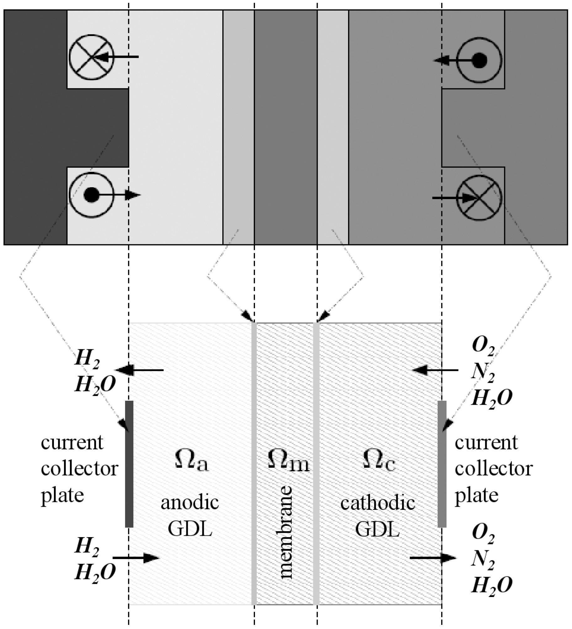
Figure 1. The pressure losses in the anode and cathode channels are neglected, that is to say that pressures at channel exits (entry of Gas diffusion layers) are equal to pressures at channel entries. Thus the computational region can be sketched as in
Figure 2 and
Figure 3.
Figure 2.
Piece of a cross section (middle) and computational region.
Figure 2.
Piece of a cross section (middle) and computational region.
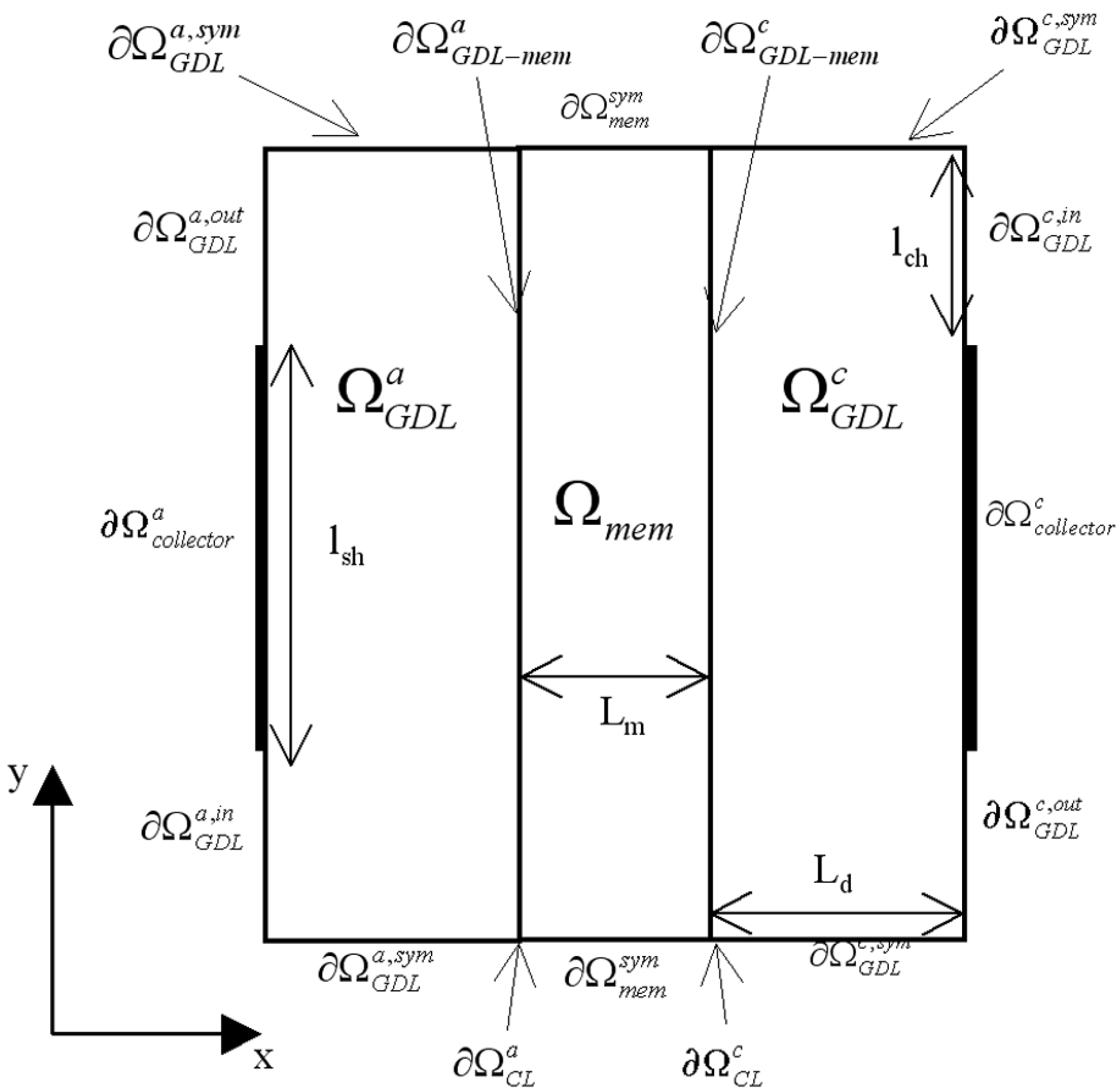
Figure 3.
Model regions () and model boundaries () definition.
Figure 3.
Model regions () and model boundaries () definition.
The models presented hereafter take into account the coupled transport processes in gas diffusion layers, in catalyst layers, and in the membrane. It is assumed that:
- (1)
water exists only in the gas phase within the electrodes, and as solute water in the membrane,
- (2)
the cell temperature remains constant and homogeneous all over the cell,
- (3)
the gas diffusion layers (GDLs) and the membrane are isotropic and homogeneous,
- (4)
the catalyst layers are very thin and are considered as reactive surfaces,
- (5)
the membrane is gas-tight,
- (6)
all electrical contact resistances are neglected,
- (7)
the current density is homogeneous at collectors.
The characteristics of the single fuel cell correspond to a commercial PEMFC made in Germany (UBZM manufacture) and are given in
Table 1.
Table 1.
Single fuel cell characteristics.
Table 1.
Single fuel cell characteristics.
| Parameter | Symbol | Value |
|---|
| GDL thicknesses | Ld | 400 μm |
| Membrane thickness | Lm | 15 μm |
| Cell active area | Acell | 100 cm2 |
| Membrane type | Gore Primea 5761 | |
| Open circuit voltage | VOC | ~1 V |
| Nominal voltage | VN | 0.6 V |
| Rated power | PN | 30 W |
2.1. Gas Diffusion Layers
The reactant gases, hydrogen and air (oxygen), flow into the fuel cell through the flow-fields. From these flow-fields, the gases diffuse through the gas diffusion layers into the catalyst layers, where electrochemical reactions occur [hydrogen oxidation (1) in the anode, and oxygen reduction (2) in the cathode]. The GDLs are made of porous carbon paper or cloth allowing simultaneous gas and liquid flows.
In this diffusion layers, two kinds of transport phenomena can be distinguished: Stefan-Maxwell diffusion, and Knudsen diffusion. They represent the collisions between molecules and molecules, and between the wall pores and molecules, respectively.
2.1.1. Charge Transport Equations
Charge transport in GDLs is governed by Ohm’s law. Thus, the electronic current density and the electrical potential are linked by:
where σ
s is the electronic conductivity of the electrodes. Charge conservation is given by:
2.1.2. Mass Transport Equations
The gas diffusion region of thickness L
d begins at x = 0 on the anode side (respectively at x = 2 L
d + L
m on the cathode side) and comes to an end at the point x = L
d (respectively at x = L
d + L
m). The interactions between a pair of species (i, j) are characterized by the binary diffusion coefficient D
ij [
18]:
where molar fractions that appear in Equation (5) are defined by:
The sum of molar fraction in the cathode and anode respectively is equal to one:
and:
Table 2 hereafter details values of
[
18]. To account for GDL porosity, the effective diffusion coefficient is calculated with Bruggeman’s relation:
Table 2.
Binary diffusivities at P
0 = 1 atm [
12].
Table 2.
Binary diffusivities at P0 = 1 atm [12].
| Diffusivity name | Ref. temperature T0 [K] | Diffusivity value [m2.s−1] |
|---|
| 307.1 | 9.15 × 10⁻⁵ |
| 308.1 | 2.82 × 10⁻⁵ |
| 293.2 | 2.20 × 10⁻⁵ |
| 307.5 | 2.56 × 10⁻⁵ |
Using the Onsager reciprocal relation [
19,
20], we also have:
is the effective diffusion coefficient between species i and the porous medium. The
are known to be independent of pressure and composition, since the species behave independently in low pressure Knudsen regime [
8]. These coefficients are then given by:
where d
p is the pore diameter, and M
i the molar mass of the specie i.
The anode and cathode pressures of the mixture denoted Pa and Pc are evaluated assuming the gas to be ideal and adiabatic.
At last, mass conservation leads to:
2.1.3. Boundary Conditions for Charge Transport
At the current collectors
and
, the electronic current density is equal to an imposed value J
cell, calculated from the whole cell current I
cell, and from the actual active area of the membrane (100 cm
2):
and
align being the outward normal vectors of GDL regions (
and
in
Figure 3). At membrane-electrode interfaces (
and
), the continuity of current density is considered, so that:
current densities j
a and j
c being given by usual electrochemical kinetics relations (Butler-Volmer equations).
Elsewhere at GDL boundaries, the normal component of current density is equal to zero. Therefore, it can be written at GDL inlets (
and
) and GDL outlets (
and
) for insulation reasons, or at boundaries
and
for symmetry reasons:
2.1.5. Equivalent Circuit Modeling of Mass Transport
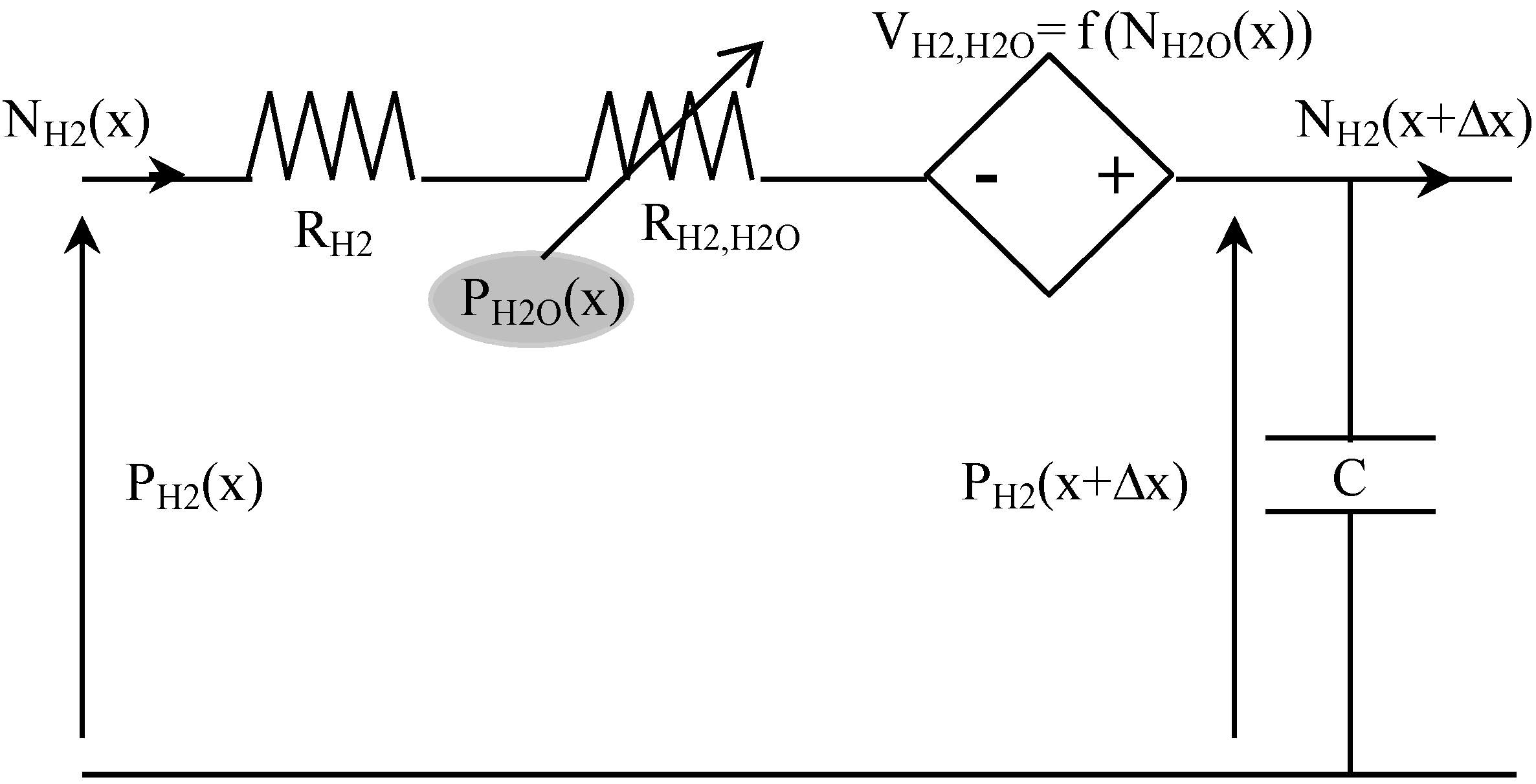
Table 3 presents some analogies between mass transport and electrical variables. For example, hydrogen transport in anode GDL can be described using the equivalent circuit shown in
Figure 4. Indeed, the Kirchhoff’s voltage law is analog to the mass transport equation [
i.e., Equation (5)], and its Kirchhoff’s current law is analog to the mass balance equation [
i.e., Equation (12)]. In this circuit, the voltage P
H2 corresponds to the partial pressure of H
2, and the current density N
H2 is the molar flow density of H
2.
Table 3.
Analogy between mechanical and electrical formulations.
Table 3.
Analogy between mechanical and electrical formulations.
| Transport model | Electrical distributed model |
|---|
| pressure: P [Pa] | voltage: U [V] |
| molar flow density: N [mol·m−2·s−1] | current density: J [A·m−2] |
| electrical resistivity: ρel [Ω·m] |
| |
| specific capacitance: cv [F·m−3] |
| |
Figure 4.
Equivalent electrical circuit for hydrogen transport in anode GDL.
Figure 4.
Equivalent electrical circuit for hydrogen transport in anode GDL.
The resistance (in Ω·m
2) is composed of a constant-value resistance R
H2 and a voltage-dependent resistance R
H2,H2O, which depends on water molar fraction:
The current-controlled voltage source V
H2,H2O depends on water molar flow density, and on hydrogen molar fraction:
At last, the capacitance C (in F·m
−2) represents the mass balance expressed in Equation (12):
A similar equivalent circuit, coupled to the previous one by partial pressures and molar flow densities, can be used for water transport in the anode GDL. Then, gas mixture diffusion in fuel cell anode is described by associating in series such equivalent coupled circuits. In the analogical model presented here, a space discretization in 10 elements of anode GDL is used (Δx = Ld/10).
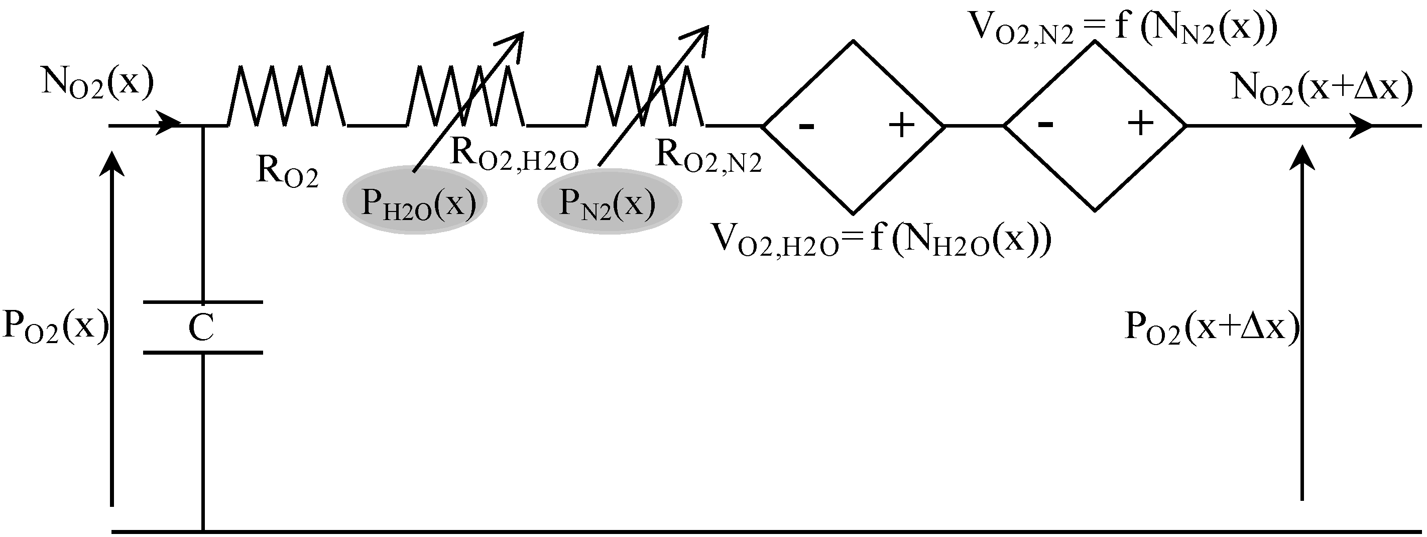
The same principle, as described above, is used to establish the equivalent electrical circuit for gas diffusion on the cathode side. This leads for oxygen to the following equivalent circuit (
Figure 5).
Figure 5.
Equivalent electrical circuit for oxygen transport in cathode GDL.
Figure 5.
Equivalent electrical circuit for oxygen transport in cathode GDL.
2.2. Membrane
The fuel cell membrane (domain ), in which water and ions are transported, contents the following unknowns: water concentration (liquid phase) CH2O, and electrolyte potential φm.
2.2.1. Charge Transport Equations
Proton transport in the membrane is governed by Ohm’s law. Thus, the ionic current density and the electrical potential are linked by:
where σ
m is the ionic conductivity of the membrane that greatly depends on the membrane hydration state. Charge conservation is given by:
2.2.2. Water Transport Equations
The water transport in the membrane is a combination of two competing diffusion mechanisms [
23,
24]. One is due to the proton displacement from the anode to the cathode. As protons are solvated, they drag some water molecules with them. This phenomenon is called electro-osmotic drag. The other mechanism is water diffusion that generally occurs from the cathode to the anode. This water flux results from the water concentration gradient created in the membrane by the electro-osmotic drag and the water produced by the redox reaction at the cathode. Therefore, the total molar flow density of water transported inside the membrane is given by:
where
is the ionic current density in the membrane, n
d is the electro-osmotic drag coefficient (number of water molecules dragged per proton), and
is the water diffusion coefficient. These coefficients depend on the membrane water content [
3]. The conservation of water quantity in the membrane can be written as:
2.2.3. Parametric Laws
The electro-osmotic drag coefficient, the water diffusion coefficient, and the membrane ionic conductivity strongly depends on membrane hydration state, which is often represented by the membrane water content λ. This quantity is defined as the ratio between the number of water molecules and the number of sulfonic sites SO
3¯ available in the polymer. It can also be stated versus membrane equivalent weight EW, membrane density ρ
m, and water concentration as follows:
In practice, water content approximately varies between 2 and 22. Springer
et al. [
25] have established the following linear empirical law for the electro-osmotic drag coefficient:
Ye
et al. have studied diffusion properties of Gore-Select
® membrane [
26], and propose for water diffusion coefficient versus water content and temperature:
Finally, we will use for the membrane ionic conductivity the following empirical law [
3,
27], available for λ > 1 only:
2.2.4. Boundary Conditions for Charge Transport
As previously in GDL regions, the continuity of current density is considered at membrane-electrode interfaces
and
, so that:
At boundaries
, the normal component of current density is equal to zero for symmetry reasons:
2.2.5. Boundary Conditions for Water Transport
At membrane-electrode interfaces
and
, the continuity of water molar flow is considered. Thus, according to relations (20) and (21), we obtain:
Boundary conditions for the membrane water content λ are defined by the sorption phenomenon that occurs at these interfaces. Therefore, they are given by:
where λ
a and λ
c are calculated versus water activity, through a linear interpolation based on the empirical sorption curves defined by Equation (19).
At last, at boundaries
, the normal component of water molar flow density is equal to zero for symmetry reasons:
2.2.6. Equivalent Circuit Modeling of Water Transport
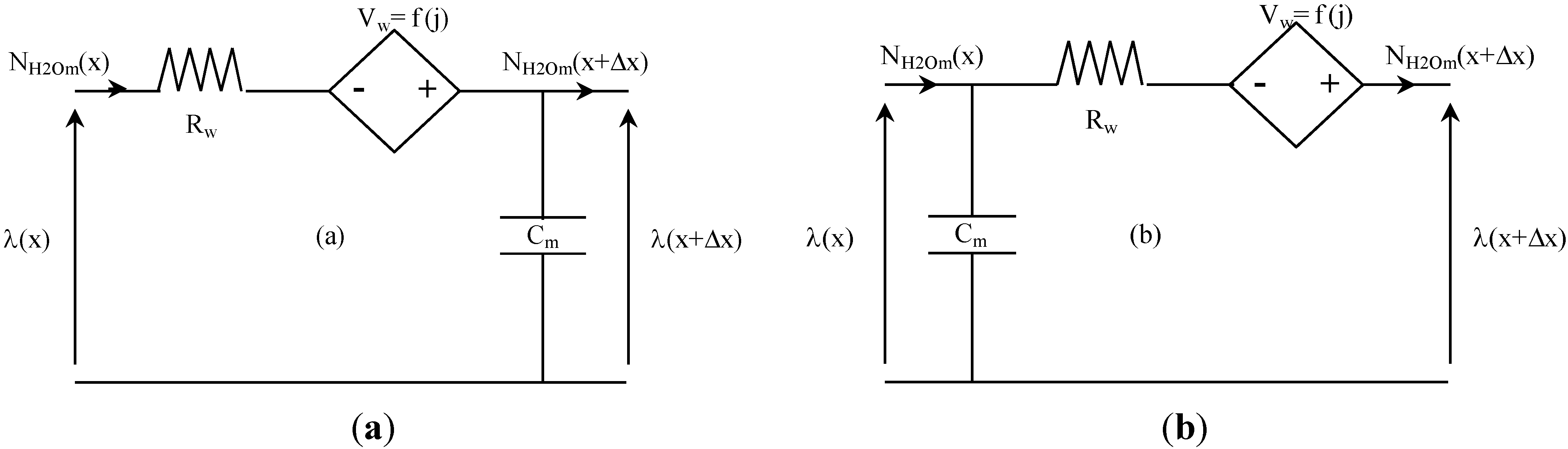
Figure 6 presents the two equivalent electrical schemes of water transport in membrane that are implemented in our model. The first (
Figure 6a) is used for the left part of the membrane (anode side), and the second (
Figure 6b) for the right part of the membrane (cathode side). Water transport in the membrane is then described by associating in series these equivalent circuits. In the analogical model presented here, a space discretization in 10 elements of the membrane (5 elements for the left part of the membrane, and as many for the right part) is used (Δx = L
m/10).
Figure 6.
Equivalent electrical circuit for water transport in the membrane.
Figure 6.
Equivalent electrical circuit for water transport in the membrane.
The resistance R
w [Ω·m
2], the current-controlled voltage source V
w [V] and the capacitance C [F·m
−2] can be established as follows, using Equations (29–31):
2.3. Catalyst Layers
The catalyst layers are very thin, so that they can be considered as reactive surfaces, denoted
and
in
Figure 3. Unknowns here are current densities j
a and j
c, which contain a faradic component governed by Butler-Volmer equations [
28]:
and a capacitive current density given by:
where c
dla and c
dlc are double layer capacitances. Therefore, the current densities in the anode and cathode active layer are the sum of these two currents:
For our 100 cm
2 Gore-type single cell, the double layer capacitance has been evaluated to 2 F, by using an impedance spectroscopy method. In Equation (41), η
a and η
c are electrode electrochemical overvoltages. They are calculated versus electrode potential and membrane potential at membrane-electrode interfaces as follows:
and being the electrode equilibrium potentials.
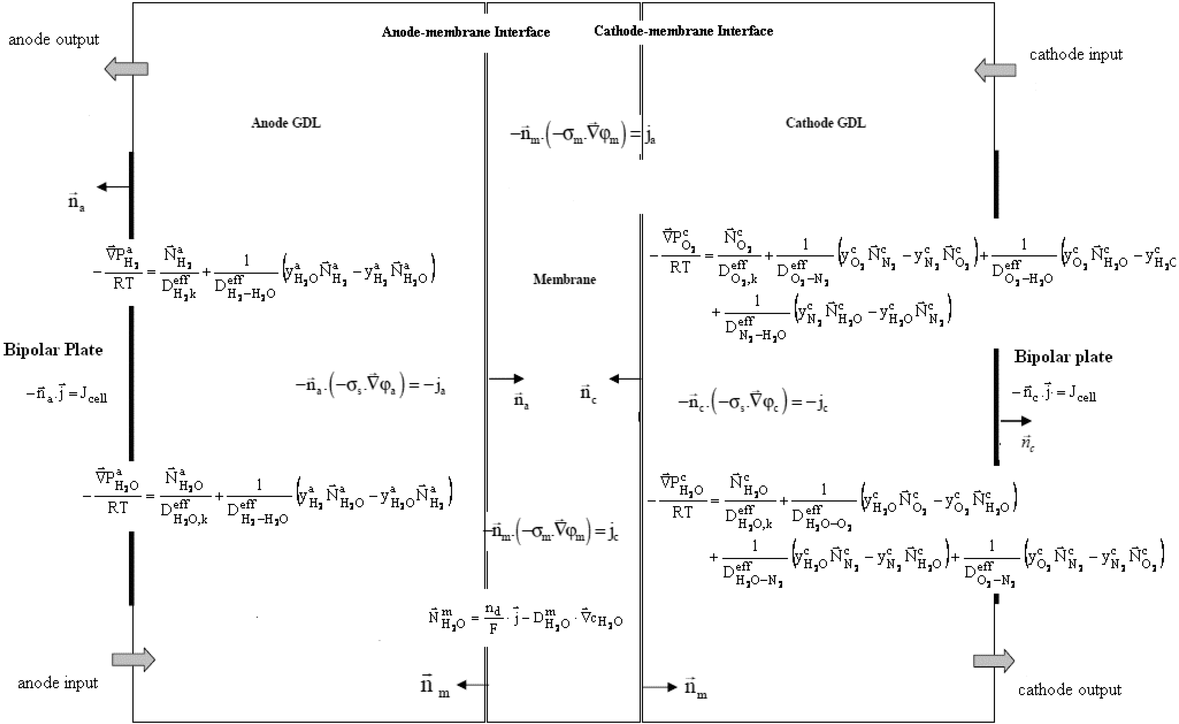
2.4. Membrane Electrodes Assembly (MEA) Model
Figure 7 presents the mathematical model as it has been implemented in COMSOL
®. Boundary conditions have not been represented, in order to make it clear.
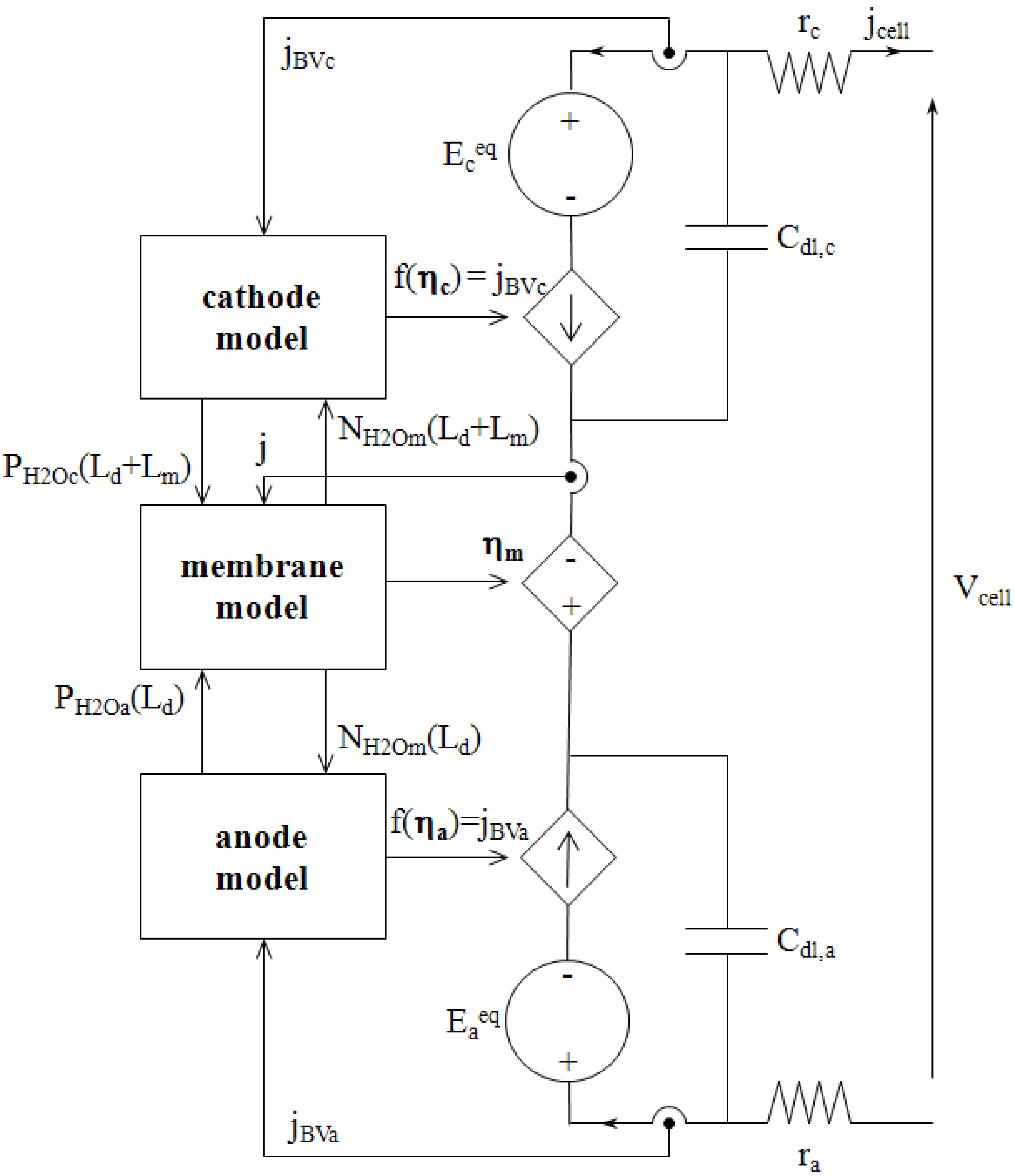
Figure 8 depicts the circuit model as it has been implemented in SABER
®.
It consists of two parts coupled to each other: analogical transport models previously described, and a standard electrical scheme that computes the fuel cell output voltage and current. It should be noticed here that we make use of voltage controlled current sources to represent the electrical laws [Equation (41)] associated with the electrochemical reactions, i.e., the links between Faraday current densities jBVa and jBVc, and electrochemical overvoltages ηa and ηc, respectively. This representation has been chosen because it respects the electrical engineering rules of source connection.
3. Numerical Simulations
To validate the circuit model, several simulations have been made and compared to the results obtained by solving the coupled PDE with Comsol Multiphysics software
® (version 3.5). Parameters required for the description of the electrochemical reaction and the water transport across the membrane are based on literature values, and are given in
Table 4. Geometric parameters and operating conditions are detailed in
Table 5 and
Table 6, respectively. First of all, polarization curves are compared. Then dynamic voltage responses to different current waveforms are plotted versus time. All initial conditions correspond to the steady state.
Figure 7.
Coupled partial differential equations of an MEA.
Figure 7.
Coupled partial differential equations of an MEA.
Figure 8.
Electrical circuit model of a single cell.
Figure 8.
Electrical circuit model of a single cell.
Table 4.
Model physic parameters.
Table 4.
Model physic parameters.
| Parameter | Symbol | Value | Unit | Ref. |
|---|
| dry GDL porosity | εs | 0.6 | - | [29] |
| dry membrane density | ρm | 2020 | kg·m−3 | [30] |
| equiv. membrane weight | EW | 0.95 | kg·mol−1 | [31] |
| anod. exch. curr. density | | 5000 | A·m−2 | [32] |
| cath. exch. curr. density | | 20 | A·m−2 | estimated |
| anod. transfer coefficient | αa | 2 | - | [32] |
| cath. transfer coefficient | αc | 0.5 | - | [32] |
| double layer capacitor | cdla, cdlc | 2 | F | measured |
Table 5.
Model geometric parameters.
Table 5.
Model geometric parameters.
| Parameter | Symbol | Value | Unit |
|---|
| inlet channel height | lch | 0.5 | mm |
| outlet channel height | lch | 0.5 | mm |
| current collector height | lsh | 1 | mm |
| GDL thickness | Ld | 400 | μm |
| membrane thickness | Lm | 15 | μm |
Table 6.
Operating conditions.
Table 6.
Operating conditions.
| Parameter | Symbol | Value | Unit |
|---|
| cell temperature | T | 333 | K |
| anode relative humidity | HRa | 0% | - |
| cath. relative humidity | HRc | 79% | - |
| anode outlet pressure | | 1.013 × 10⁵ | Pa |
| cathode outlet pressure | | 1.013 × 10⁵ | Pa |
3.1. In Steady State
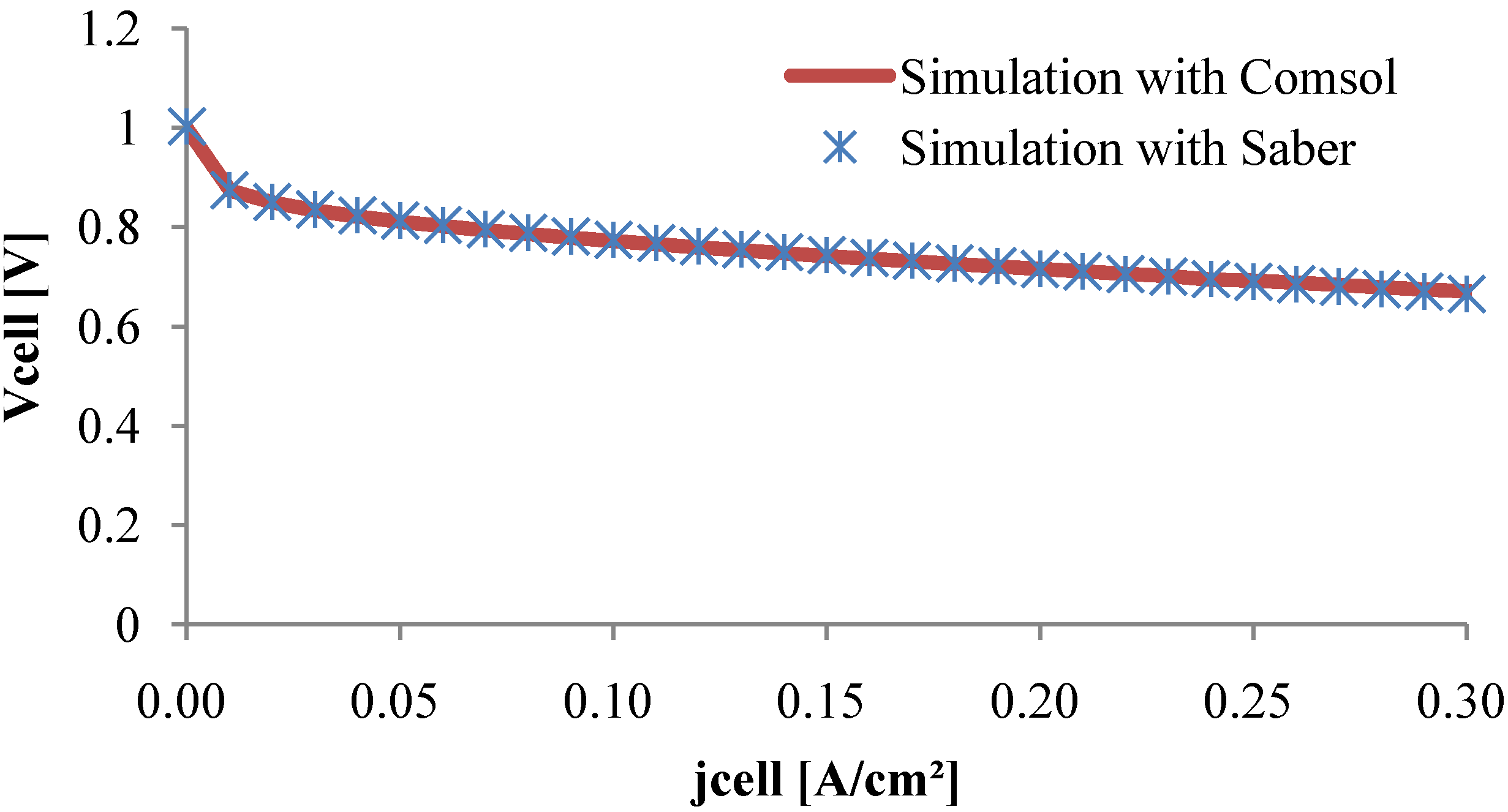
As it can be seen in
Figure 9, the polarization curve obtained with the equivalent electrical model fits the Comsol
® plotted curve in a large current density scale. Thus, the circuit model seems to be in good agreement with the PDE model.
Figure 9.
Polarization curve.
Figure 9.
Polarization curve.
3.2. In Transient State
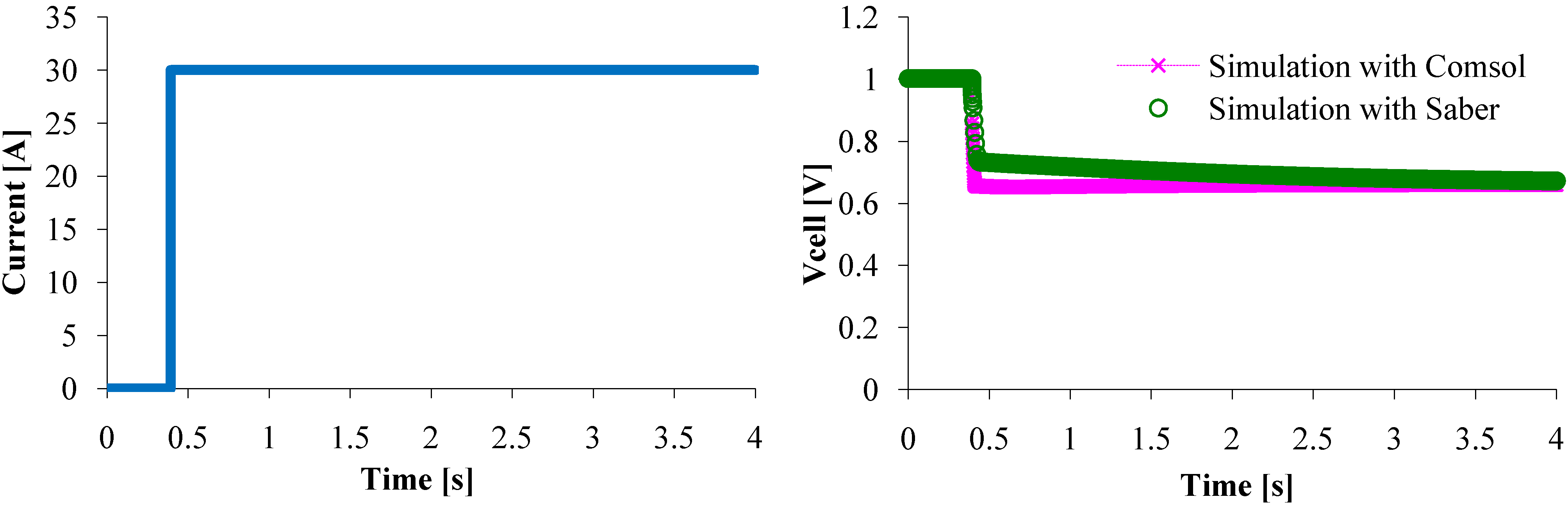
Now, we have to check if the model can effectively represent the dynamic behavior of a single PEM fuel cell that has a sudden change load current, for example a 30 A step current (
Figure 10). The voltage responses are exactly the same when the steady state is reached, however a little difference can be pointed out while current increased from 0 to 30 A. This difference might be due to the computational domain. Indeed, even if the PDE model is one dimension (as the circuit model), the computational domain is 2D as it can be seen in
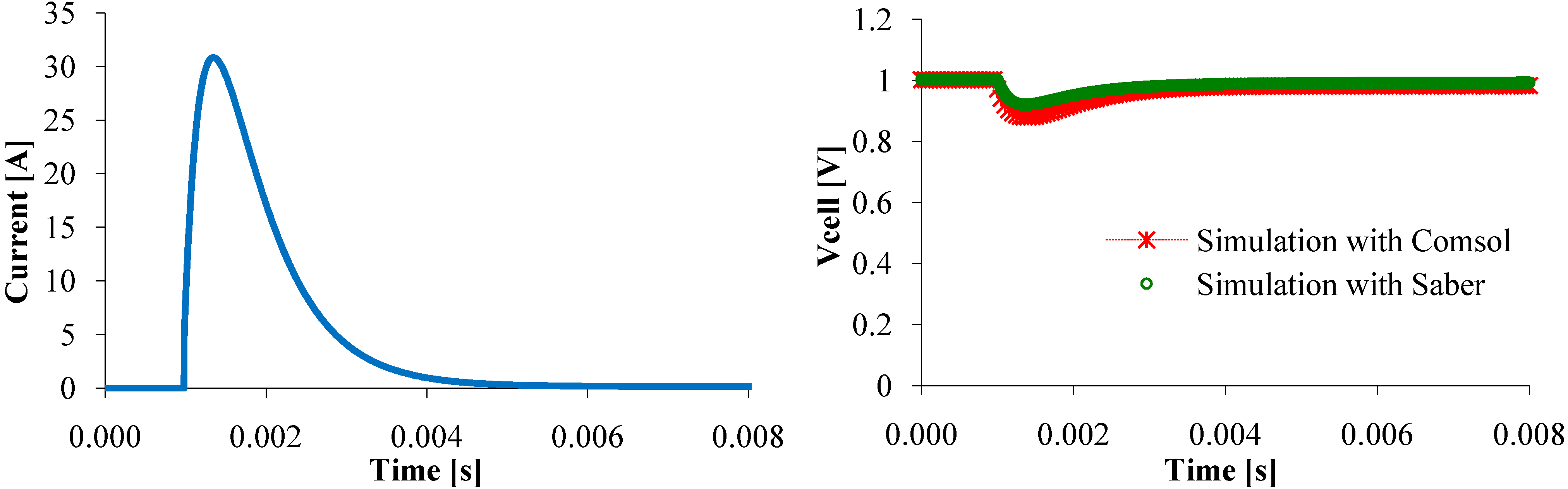
Figure 7. Therefore, in transient state, some parameters assumed to be constant along (Oy) axis might vary, that cannot happen with the circuit model. This difference reduces when the current change is just a little smooth (
Figure 11). So, the circuit model represents as well as the mathematical model the steady state and the dynamic PEMFC behavior.
Figure 10.
Fuel cell voltage response to a 0–30 A current step.
Figure 10.
Fuel cell voltage response to a 0–30 A current step.
Figure 11.
Voltage response to a current peak.
Figure 11.
Voltage response to a current peak.
3.3. Practical Application
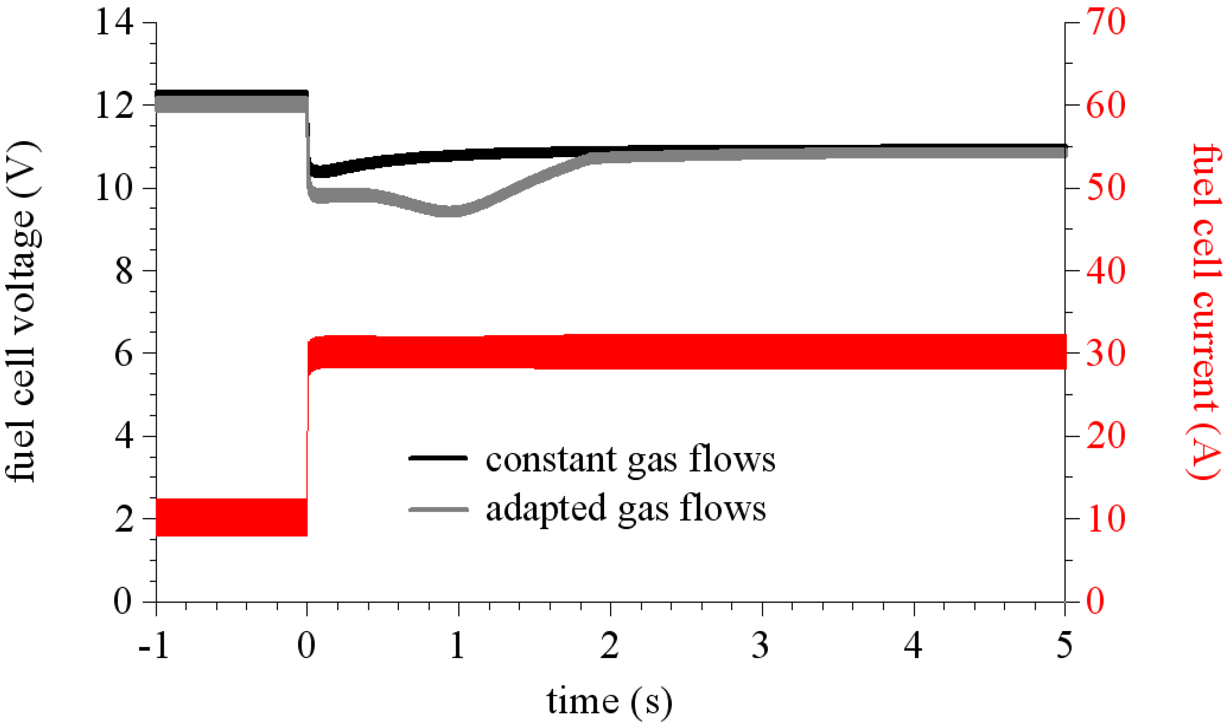
To illustrate the use of our model in a practical system, we simulate the association of a fuel cell stack and a current regulated boost converter. The stack is composed of 16 cells of 100 cm2 active area and the boost switching frequency is 10 kHz. We assume that the stack model is the same as the cell model; therefore we just have to multiply the results by the cell number of the stack.
We study two different ways to feed the stack. The first one corresponds to a constant gas flow rate, it means that the gas flow rates are independent of the fuel cell current, we just take care to overfeed the stack for example as if the current could reach Iref = 40 A (where Iref is the setpoint used to compute the gas flow rates). The second way is called adapted gas flows. In this case, the fuel cell current is used to compute the gas flow rates [Iref = Icell (t)].
Figure 12 shows calculated voltage responses of the stack to a current step (10 A/30 A) in these two gas flow conditions. As it can be seen, in the case of an overfed stack the voltage drops slightly under its final value. Whereas when the stack runs under adapted flow conditions, the voltage drops far from its final steady state value then increases to reach its steady state. This phenomenon is called fuel or air starvation that occurs during fast power demands (such as current steps), when gas flows are set by current level. This is mainly due to the slow time constant of the air flux controller. This time constant was measured to 1 second in our test bench.
Figure 12.
Simulated responses to a 10 A/30 A current step of a fuel cell stack connected to a regulated boost converter.
Figure 12.
Simulated responses to a 10 A/30 A current step of a fuel cell stack connected to a regulated boost converter.
An interesting comment to make on these simulation results is that they also allow us to obtain the membrane resistance. Indeed, due to the sufficiently high switching frequency by dividing the voltage ripple by the current ripple, the membrane resistance values are obtained around the operating point.

