Fatigue Reliability and Calibration of Fatigue Design Factors for Offshore Wind Turbines

Abstract

Consequences of failure of offshore wind turbines (OWTs) is in general lower than consequences of failure of, e.g., oil & gas platforms. It is reasonable that lower fatigue design factors can be applied for fatigue design of OWTs when compared to other fixed offshore structures. Calibration of appropriate partial safety factors/Fatigue Design Factors (FDF) for steel substructures for OWTs is the scope of this paper. A reliability-based approach is used and a probabilistic model has been developed, where design and limit state equations are established for fatigue failure. The strength and load uncertainties are described by stochastic variables. SN and fracture mechanics approaches are considered for to model the fatigue life. Further, both linear and bi-linear SN-curves are formulated and various approximations are investigated. The acceptable reliability level for fatigue failure of OWTs is discussed and results are presented for calibrated optimal fatigue design factors. Further, the influence of inspections is considered in order to extend and maintain a given target safety level.

1. Introduction

Consequences of failure of the support structure of an offshore wind turbine are in general lower than consequences of failure of, e.g., oil & gas platforms. The support structure for offshore wind turbines contributes with a substantial part of the total cost of an offshore wind farm. Therefore, in order to increase the competitiveness of offshore wind energy compared to other energy supply methods it is important to minimize the cost of energy considering the whole life cycle. In traditional deterministic, code-based design, the structural costs are among other things determined by the value of the safety factors, which reflects the uncertainty related to the design parameters. Improved design with a consistent reliability level for all components can be obtained by use of probabilistic design methods, where explicit account of uncertainties connected to loads, strengths and calculation methods is made. In probabilistic design the single components are designed to a level of safety, which accounts for an optimal balance between failure consequences, material consumption and the probability of failure. For instance, manned offshore steel jacket structures for oil & gas production are typically designed to fulfill a requirement to the maximum annual probability of failure of the order 10⁻⁵. For unmanned structures a maximum annual probability of failure is typically 10⁻⁴, see DNV-RP-C203 [1]. For offshore wind turbines a reliability level corresponding to unmanned structures or even lower can be relevant. This implies possibilities for cost reductions. Further, if inspections are performed even lower material costs can be obtained, but they have to be balanced with the costs to inspections. Such a reliability- and risk-based approach has been used for offshore oil & gas steel structures, see, e.g., Faber et al. [2] and Moan [3]. In this paper the reliability-based approach is used for support structures for offshore wind turbines, see also Sørensen [4].

Design equations to be used for deterministic, code-based design and corresponding limit state equations to be used for reliability assessment are formulated. In the limit state equations uncertain parameters are modeled as stochastic variables. In the design equations safety factors for fatigue strength and load or equivalently Fatigue Design Factors (FDF) are used to secure the required reliability level. SN-curves and Miner’s rule with linear damage accumulation are used as recommended in most relevant standards. SN-curves and Miner’s rule are used as basis for reliability assessment by the SN-approach, see Section 2 and a fatigue assessment by Fracture Mechanics approach is used for reliability assessment taking into account inspections, see Section 4. In Section 3 the minimum acceptable reliability level is discussed. Requirements to fatigue design factors for design of welded details in support structures for offshore wind turbines are presented in Section 5, both without and with inspections.

2. Reliability Modelling of Fatigue Failure Using the SN-Approach

In this section how the reliability of the fatigue critical details can be performed using the SN-approach with SN-curves in combination with the Miner’s rule as generally recommended in codes and standards, e.g., EN 1993-1-9 [5], IEC 61400-1 [6], DNV [7] and GL [8] is described.

If a bilinear SN-curve is applied the SN relation can be written:

$$N=K_1{\left(\mathrm{\Delta }s{\left(\frac{T}{T_{ref}}\right)}^{\alpha }\right)}^{-m_1}\mathrm{for}N\le N_C$$

(1)

$$N=K_2{\left(\mathrm{\Delta }s{\left(\frac{T}{T_{ref}}\right)}^{\alpha }\right)}^{-m_2}\mathrm{for}N>N_C$$

(2)

where:

K1, m1	Material parameters for N ≤ NC
K2, m2	Material parameters for N > NC
Δs	Stress range
N	Number of cycles to failure
T	Material thickness
Tref	Reference thickness
α	Scale exponent

Further, it is assumed that the total number of stress ranges for a given fatigue critical detail can be grouped in n_σ groups/intervals such that the number of stress ranges in group i is n_i per year. (ΔQ_i, n_i) is obtained by Rainflow counting and can e.g. be represented by “Markov matrices”. The code-based design equation using the Miner’s rule is written:

$$G=1-{\displaystyle \sum _{s_i\ge \mathrm{\Delta }{s}_C}\frac{n_i{T}_F}{K_1^C{s}_i^{-m_1}}}-{\displaystyle \sum _{s_i<\mathrm{\Delta }{s}_C}\frac{n_i{T}_F}{K_2^C{s}_i^{-m_2}}}=0$$

(3)

where:

KiC	Characteristic value of Ki (logKiC equal to the mean of logKi minus two standard deviations of logKi)
$s_i=\frac{\mathrm{\Delta }{Q}_i}{z}{\left(\frac{T}{T_{ref}}\right)}^{\alpha }$	Stress range in group i
ΔQi	Action effect (proportional to stress range si in group i)
z	Design parameter, e.g., a cross-sectional parameter
TF	Fatigue life

As safety factor for fatigue design the Fatigue Design Factor (FDF) value can be used:

$$FDF=\frac{T_F}{T_L}$$

(4)

where T_L is the design life, typically 25 years for offshore wind turbines. Note that for a linear SN-curve with slope m the FDF value is connected to partial safety factors for fatigue load, γ_f and fatigue strength, γ_m by $FDF={\left({\gamma }_f{\gamma }_m\right)}^m$.

The probability of failure (and the corresponding reliability index) is calculated using the design value z determined from (3) and a limit state equation associated with (3). The limit state equation is written:

$$g\left(t\right)=\mathrm{\Delta }-{\displaystyle \sum _{s_i\ge \mathrm{\Delta }{s}_C}\frac{n_{i}t}{K_1{s}_i^{-m_1}}}-{\displaystyle \sum _{s_i<\mathrm{\Delta }{s}_C}\frac{n_{i}t}{K_2{s}_i^{-m_2}}}$$

(5)

where:

Δ	Model uncertainty related to Miner’s rule for linear damage accumulation. Δ is assumed Log-Normal distributed with mean value = 1 and coefficient of variation COVΔ
$s_i=X_W{X}_{SCF}\frac{\mathrm{\Delta }{Q}_i}{z}{\left(\frac{T}{T_{ref}}\right)}^{\alpha }$	Stress range for group i
XW	Stochastic variable modelling the uncertainty related to determination of loads. XW is assumed Log-Normal distributed with mean value = 1 and coefficient of variation = COVW
XSCF	Stochastic variable modelling the uncertainty related to determination of stresses given fatigue loads. XSCF is assumed Log-Normal distributed with mean value = 1 and coefficient of variation = COVSCF
Ki	LogKi is modeled by a Normal distributed stochastic variable according to a specific SN-curve
t	Time (0 ≤ t ≤ TL)

The above probabilistic model for a bilinear SN-curve can easily be simplified for a linear SN-curve with parameters m and K. It is noted that the probabilistic model is based on the assumption that the average variation in stress ranges from year to year is negligible. Even though the wind and wave loads will have some variation in average level from year to year it can be expected that due to the effect of the control system the average variation in stress ranges from year to year will be small.

The cumulative (accumulated) probability of failure in the time interval [0, t] is obtained by:

$$P_F\left(t\right)=P\left(g\left(t\right)\le 0\right)$$

(6)

The probability of failure can be estimated by FORM/SORM techniques or simulation, see Madsen et al. [9] and Sørensen [10]. The reliability index, β(t) corresponding to the cumulative probability of failure, P_F(t) is defined by:

$$\beta \left(t\right)=-{\mathrm{\Phi }}^{-1}\left(P_F\left(t\right)\right)$$

(7)

where Φ( ) is the standardized Normal distribution function. Reliability indices 3.1 and 3.7 correspond to probability of failures equal to 10⁻³ and 10⁻⁴.

The annual probability of failure is obtained from:

$$\mathrm{\Delta }{P}_F\left(t\right)=P_F\left(t\right)-P_F\left(t-\mathrm{\Delta }t\right),t>\text{ 1 year}$$

(8)

where Δt = 1 year.

Three representative SN-curves are considered, corresponding to the “D”-curve in DnV-C203 [1]:

• One for a fatigue critical detail in air,
• One for a fatigue critical detail in marine conditions with cathodic protection, and
• One for a fatigue detail subject to free corrosion

Table 1 shows a representative stochastic model that can be used in reliability assessment. A range of coefficients of variation for the stochastic variables are specified in order to cover the range of uncertainties that can be expected in practical applications. The values in bold are considered as the base case values in the assessment of required FDF values below.

The COV values for X_SCF and X_W should be associated with specific recommendations for how detailed the estimation of stress concentration factors and wind/wave loads should be made.

The coefficient of variation of the model uncertainty associated with Miner’s rule, COV_Δ and the standard deviation of logK₁ and logK₂ follows the recommendations in DnV-C203 [1]. It is noted that the uncertainties related to Δ and logK_i should be modeled carefully. The uncertainty related to Δ (variable amplitude loading and linear damage accumulation by Miner’s rule) can be significant.

Table 1. Example of stochastic model. D: Deterministic, N: Normal, LN: LogNormal.

Variable	Distribution	Expected value	Standard deviation	Characteristic value	Comment
Δ	LN	1	0.1/0.2/0.3	1
XSCF	LN	1	0.05/0.10/0.15 /0.20	1
XW	LN	1	0.10/0.20/0.30	1
m1	D	3
logK1	N	12.564	0.10/0.15/0.2	12.164	In air
logK1	N	12.164	0.10/0.15/0.2	11.764	With cathodic protection
logK1	N	12.087	0.10/0.15/0.2	11.687	Free corrosion
m2	D	5
logK2	N	16.106	0.15/0.2/0.25	15.606	In air
logK2	N	16.106	0.15/0.2/0.25	15.606	With cathodic protection
logK2		-			Free corrosion

logK₁ and logK₂ are assumed fully correlated.

Table 1. Example of stochastic model. D: Deterministic, N: Normal, LN: LogNormal.

Variable	Distribution	Expected value	Standard deviation	Characteristic value	Comment
Δ	LN	1	0.1/0.2/0.3	1
XSCF	LN	1	0.05/0.10/0.15 /0.20	1
XW	LN	1	0.10/0.20/0.30	1
m1	D	3
logK1	N	12.564	0.10/0.15/0.2	12.164	In air
logK1	N	12.164	0.10/0.15/0.2	11.764	With cathodic protection
logK1	N	12.087	0.10/0.15/0.2	11.687	Free corrosion
m2	D	5
logK2	N	16.106	0.15/0.2/0.25	15.606	In air
logK2	N	16.106	0.15/0.2/0.25	15.606	With cathodic protection
logK2		-			Free corrosion

logK₁ and logK₂ are assumed fully correlated.

3. Acceptable Reliability Level for Fatigue Failure

The minimum required reliability level for offshore wind turbines can be assessed by different considerations. For manned and unmanned offshore steel jacket structures for oil & gas production maximum annual probabilities of failure of the order 10⁻⁵ (reliability index equal to 4.3) and 10⁻⁴ (reliability index equal to 3.7) are generally accepted, see, e.g., DnV-C203 [1]. No explicit reference exists for the minimum reliability index required for the partial safety factors in IEC 61400-3:2009 [11] for offshore wind turbines. However, the implicit reliability level in the standards used for design of offshore wind turbines by DNV [7] and GL [8] can alternatively be estimated using the stochastic model presented in Section 2 together with the partial safety factors recommended in these standards. The First Order Reliability Method (FORM) was used and verified with Monte Carlo Simulations (MCS) in order to calculate the reliability indices obtained using the stochastic model proposed in Section 2.

Table 2 shows required FDF (Fatigue Design Factors) values for fatigue design in the documents:

• Design of fixed offshore steel structures for oil & gas platforms: NORSOK, [12] and ISO 19902, [13].
• Offshore wind turbines: GL Guideline for the certification of offshore wind turbines, [8] and DNV Design of offshore wind turbine structures, DNV-OS-J101, [7].

The FDF values in Table 2 for GL/DNV are determined using a linear SN-curve with slope equal to 3 whereas the required values for FDF obtained corresponding to a slope equal to 5 are shown in ( ). The FDF values are specified for critical and non-critical details and for details than can or cannot be inspected. As expected the required FDF values for offshore oil & gas platforms are higher than for offshore wind turbines.

Table 2. Fatigue Design Factors (FDF) required.

Failure critical detail	Inspections	ISO 19902	GL/DNV
Yes	No	10	2.0 (3.0)
Yes	Yes	5	1.5 (2.0)
No	No	5	1.5 (2.0)
No	Yes	2	1.0 (1.0)

Table 2. Fatigue Design Factors (FDF) required.

Failure critical detail	Inspections	ISO 19902	GL/DNV
Yes	No	10	2.0 (3.0)
Yes	Yes	5	1.5 (2.0)
No	No	5	1.5 (2.0)
No	Yes	2	1.0 (1.0)

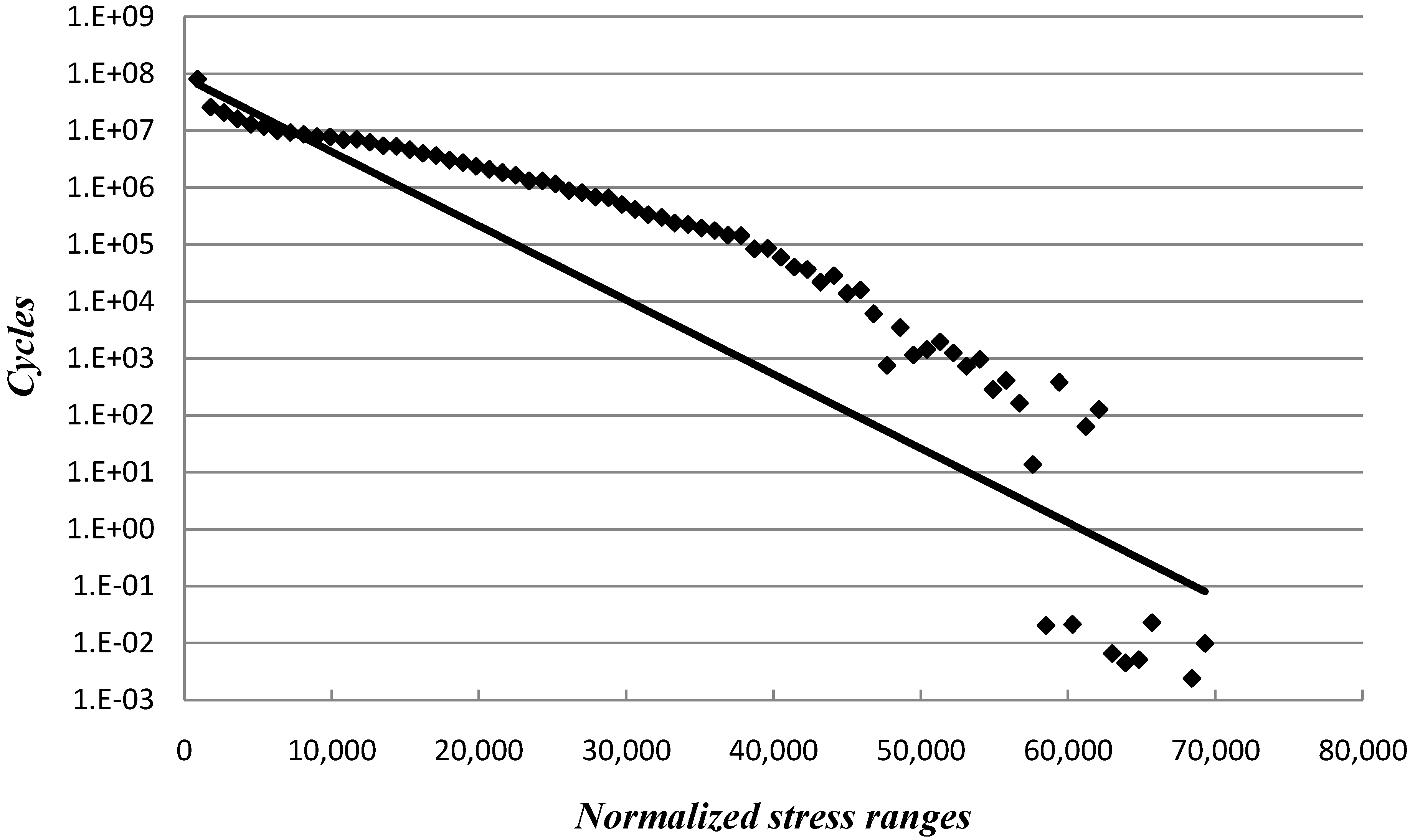
A representative distribution of the number of stress ranges as function of stress ranges from a typical 2.3 MW offshore wind turbine is used in order to assess the acceptable reliability level for fatigue failure, see Figure 1. The number of stress cycles per year is approximately 3.5 × 10⁷. A linearized approximation of the stress distribution, which is characterized by the straight line, is also considered in order to illustrate the importance of the choice of stress range distribution, see Section 5.1.

Table 3 shows the cumulative and annual reliability indices obtained with a design lifetime equal to 25 years, the stress range distribution in Figure 1, Fatigue Design Factors (FDF) corresponding to those specified in Table 2 and using the stochastic models and SN-curves in Table 1. It is seen that for bilinear SN-curves (“In air” and “With cathodic protection”) the cumulative and annual reliability indices corresponding to FDF = 3 are 2.5 and 3.1 whereas for linear SN-curves (“Free corrosion”) the cumulative and annual reliability indices corresponding to FDF = 3 are larger. Further, it is seen that the required reliability level (with the stochastic model in Table 1) is smaller than the reliability level corresponding to un-manned offshore platforms.

In assessment of the consequences of failure of a fatigue critical detail different system effects can additionally be important:

• Mechanical load re-distribution may imply larger fatigue loads on other critical details.
• The directional distribution of wind speeds should be taken into account when assessing the fatigue load for the individual fatigue critical details. Using an omnidirectional distribution of wind speeds could be too conservative.
• Probabilistic parallel system effect may be important since failure of one detail does not necessarily imply total failure/collapse.

Figure 1. Representative model and linearized model for number of stress ranges as function of stress ranges (normalized).

Figure 1. Representative model and linearized model for number of stress ranges as function of stress ranges (normalized).

Table 3. Reliability indices for different FDF values. xx/yy indicates reliability indices corresponding to cumulative and annual probability of failure, respectively.

FDF	In air	With cathodic protection	Free corrosion
1.0	1.3/2.4	1.2/2.4	1.3/2.3
2.0	2.0/2.8	1.9/2.8	2.3/3.0
3.0	2.5/3.1	2.4/3.1	2.9/3.4

Table 3. Reliability indices for different FDF values. xx/yy indicates reliability indices corresponding to cumulative and annual probability of failure, respectively.

FDF	In air	With cathodic protection	Free corrosion
1.0	1.3/2.4	1.2/2.4	1.3/2.3
2.0	2.0/2.8	1.9/2.8	2.3/3.0
3.0	2.5/3.1	2.4/3.1	2.9/3.4

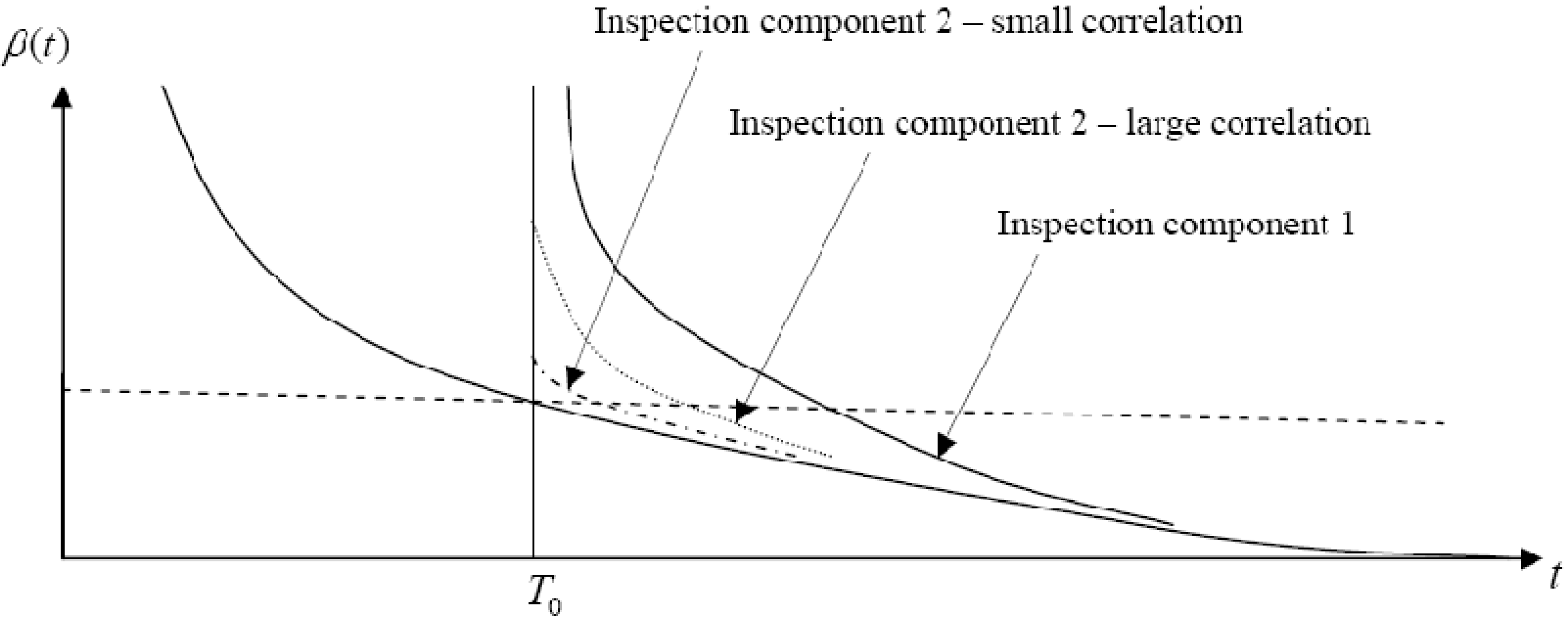
Another type of system effect can be used in a reliability assessment if inspections are performed. Due to correlations between different critical details in one wind turbine and between wind turbines in a wind farm, information from inspection of one detail can also be used to update the reliability of wind turbines that are not inspected, as illustrated in Figure 2, where updated reliability indices are shown for component 1 if an inspection is made at time T₀ of component 1 or of another component 2 with small or large correlation with component 1.

Based on the above considerations an acceptable reliability level to be used for assessment of required FDF values is chosen to correspond to accumulated reliability indices of 2.5 and 3.1 and to annual reliability indices equal to 3.1 and 3.7. These choices cover the range of reliability levels implicitly given in relevant standards.

If the fatigue detail can be characterized as being “not critical”, i.e., load bearing capacity exists after fatigue failure, then the reliability requirements can be lowered by approximately 0.5 based on the lower safety factors in GL/DNV.

Figure 2. Illustration of updating of the reliability of a critical detail/component by inspection of the same component and by inspection of another component in the same wind turbine or in another wind turbine in a wind farm.

Figure 2. Illustration of updating of the reliability of a critical detail/component by inspection of the same component and by inspection of another component in the same wind turbine or in another wind turbine in a wind farm.

4. Reliability Assessment Taking into Account Inspections

For offshore oil & gas offshore structures inspections of fatigue critical details are often performed in order to secure a sufficient reliability level. For offshore wind turbines with steel substructures it could also be considered to perform inspections during the lifetime. The costs of these inspections and possible repairs in case of detected fatigue cracks should be compensated by cheaper initial costs due to lower FDF values. In this section is described the basis for reliability- and risk-based inspection planning and they influence the reliability level.

4.1. Reliability-Based Inspection Planning

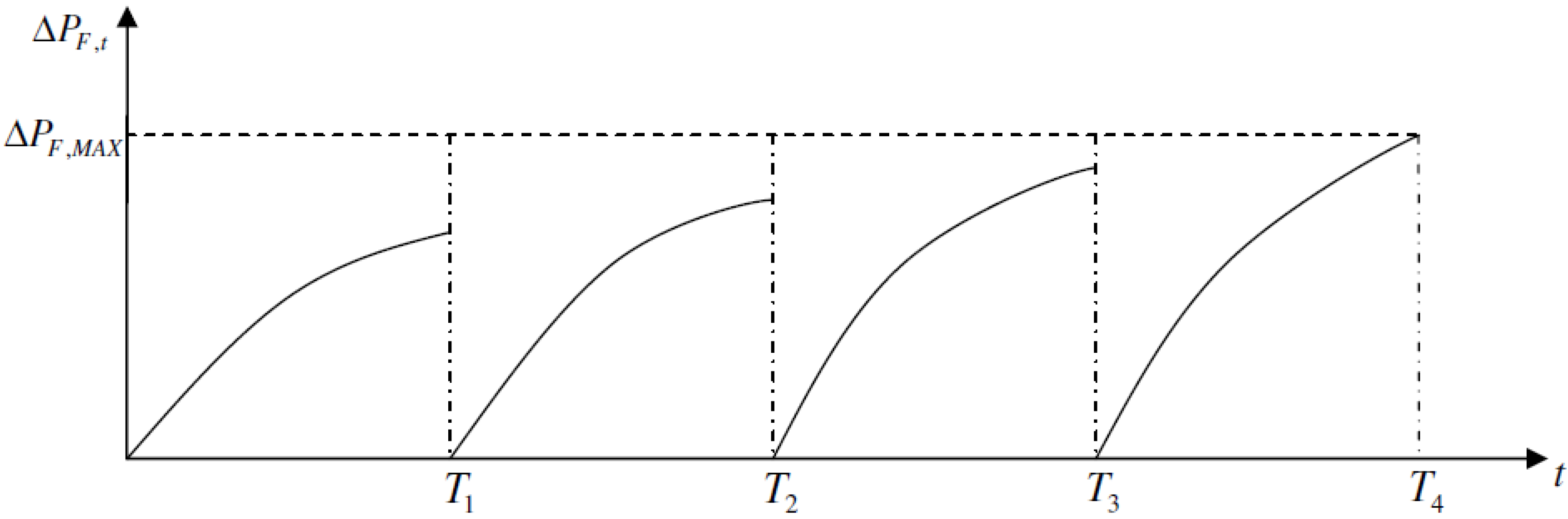
Inspection planning can be based on the requirement that the annual probability of failure in all years has to satisfy the reliability constraint:

$$\mathrm{\Delta }{P}_F\left(t\right)\le \mathrm{\Delta }{P}_{F,MAX},0\le t\le T_L$$

(9)

where ΔP_F,MAX is the maximum acceptable annual probability of failure. A similar requirement can be formulated based on the cumulative probability of failure:

$$P_F\left(T_L\right)\le P_{F,MAX}$$

(10)

The planning is often made with the assumption that no cracks are found at the inspections. However, if a crack is found, then a new inspection plan has to be made based on the observation.

If all inspections are made with the same time intervals, then the annual probability of fatigue failure could be as illustrated in Figure 3.

Figure 3. Illustration of inspection plan with equidistant inspections.

Figure 3. Illustration of inspection plan with equidistant inspections.

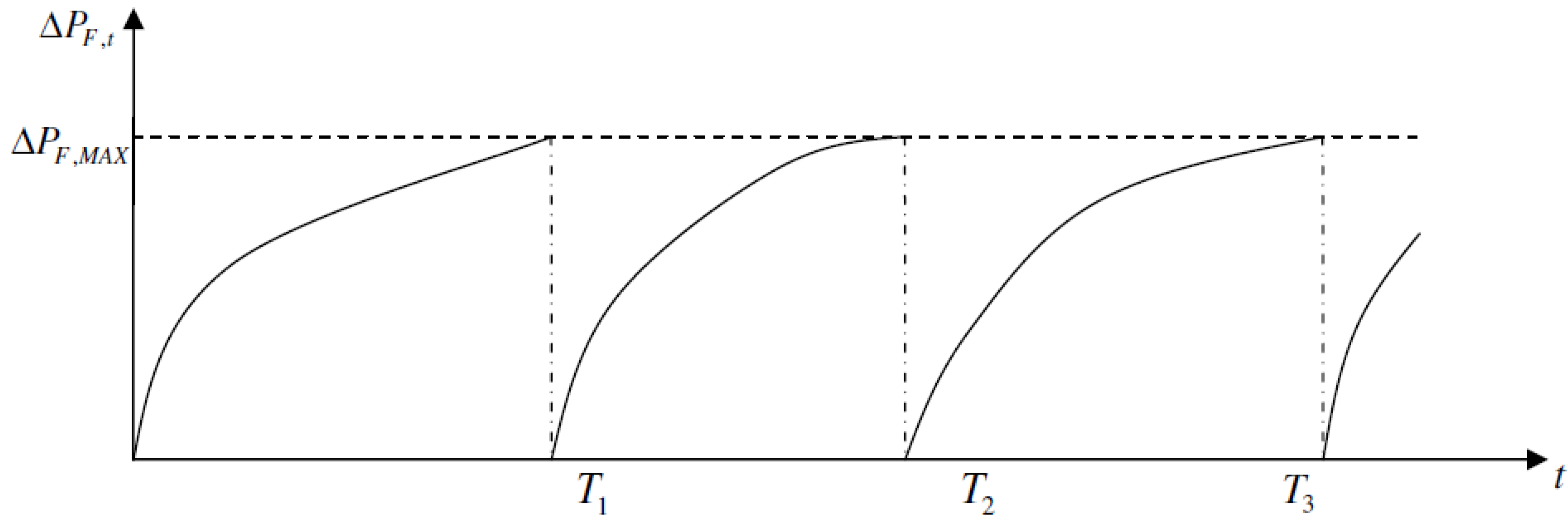
If inspections are made when the annual probability of fatigue failure exceeds the critical value then inspections are made with different time intervals, as illustrated in Figure 4. Often this approach results in increasing time intervals between inspections.

Figure 4. Illustration of inspection plan where inspections are performed when the annual probability of failure exceeds the maximum acceptable annual probability of failure.

Figure 4. Illustration of inspection plan where inspections are performed when the annual probability of failure exceeds the maximum acceptable annual probability of failure.

The inspection planning procedure described above does not take into account the costs of inspections, repairs and failures. In risk-based inspection planning these costs are taken into account. Compared to the information needed in reliability-based inspection planning the following additional information is needed:

• A decision rule to be used in connection with inspections. The decision rule should specify the action to be taken of a crack is detected, this could be do nothing, grinding, repair by welding, replacement, etc.
• Costs of inspections
• Costs of repairs
• Costs of failure
• Discounting

Further, a model is needed for estimating the probability of collapse (total failure) given fatigue failure of the detail considered.

The theoretical basis for risk-based planning of inspection and maintenance for fatigue critical details and for applications in offshore steel substructures is described in e.g., Faber et al. [2], Moan [3], Madsen and Sørensen [14], Skjong [15], Straub [16] and Sørensen [17]. Fatigue reliability analysis of jacket-type offshore wind turbine considering inspection and repair is also considered in Dong et al. [18] and Rangel-Ramírez and Sørensen [19].

For an existing structure the reliability can be updated based on the available information. The following types of information can be used: if an inspection has been performed at time T_I and no cracks are detected then the probability of failure can be updated. In order to model no-detection event a limit state equation modelling the crack growth and a model for the reliability of the inspection method, e.g., by a Probability-Of-Detection (POD)-curve is needed, see below.

4.2. Fatigue Assessment by Fracture Mechanics Approach

A Fracture Mechanical (FM) modelling of the crack growth can be applied to model the fatigue failure. 1- or 2-dimensional models can be used depending on the fatigue critical detail. The approach is that the FM model is calibrated such that it results in the same reliability level as obtained using the SN-approach described in Section 2.

In the following it is assumed that the crack can be modeled by a “1.5”-dimensional semi-elliptical crack. Since the fatigue cracks are assumed to be initiated in welded details it is assumed that the crack initiation life is negligible compared to the crack propagation life N_P.

The following 1-dimensional crack growth model is used for the crack depth a as function of number of cycles N:

$$\frac{da}{dN}=C{\left(\mathrm{\Delta }K\left(a\right)\right)}^m,a\left(0\right)=a_0$$

(11)

where C and m are constants and a₀ is the initial crack depth. The stress intensity range is obtained from

$$\mathrm{\Delta }K\left(a\right)=Y\mathrm{\Delta }{\sigma }_e\sqrt{\pi a}$$

(12)

where Y is geometry function (assumed to be a constant =1). Δσ_e is an equivalent stress range determined from:

$$\mathrm{\Delta }{\sigma }_e={\left(\frac{1}{n}{\displaystyle \sum _{i=1}^n\mathrm{\Delta }{\sigma }_i^m}\right)}^{1/m}$$

(13)

and n is the total number of stress cycles and Δσ_e , i = 1, n are the stress ranges.

The crack width 2c is assumed to be obtained from the following model for a/2c as a function of the relative crack depth a/T:

$$\frac{a}{2c}=f\left(\frac{a}{T}\right)$$

(14)

Specific models for the stress intensity ranges ΔK(a) for 1- and 2-dimensional models can, e.g., be found in BS 7910 [20] for a number of different geometries and loading conditions.

The stress range Δσ is obtained from:

$$\mathrm{\Delta }\sigma =X_W{X}_{SCF}\cdot Y\cdot \mathrm{\Delta }{\sigma }^e$$

(15)

A representative stochastic model is shown in Table 4, partially based on BS 7910 [20].

Table 4. Uncertainty modelling used in the fracture mechanical reliability analysis. D: Deterministic, N: Normal, LN: LogNormal.

Variable	Dist.	Expected value	Standard deviation
a0	LN	0.2 mm	0.132 mm
lnC	N	μlnC (reliability based fit to SN approach)	0.77
m	D	m-value (reliability based fit to SN approach)
XSCF	LN	1	See Table 1
XW	LN	1	See Table 1
n	D	Total number of stress ranges per year
aC	D	T (thickness)
Y	LN	1	0.1

Table 4. Uncertainty modelling used in the fracture mechanical reliability analysis. D: Deterministic, N: Normal, LN: LogNormal.

Variable	Dist.	Expected value	Standard deviation
a0	LN	0.2 mm	0.132 mm
lnC	N	μlnC (reliability based fit to SN approach)	0.77
m	D	m-value (reliability based fit to SN approach)
XSCF	LN	1	See Table 1
XW	LN	1	See Table 1
n	D	Total number of stress ranges per year
aC	D	T (thickness)
Y	LN	1	0.1

The limit state equation can be written in terms of number of cycles to failure:

$$g\left(X\right)=N_P-nt$$

(16)

where t is time in the interval from 0 to the service life T_L.

Equivalently, the limit state equation can be written in terms of crack depth:

$$g\left(X\right)=a_c-a\left(t\right)$$

(17)

where a(t) is the crack depth at time t and a_C is the critical crack depth, typically the thickness T.

In reliability-based inspection planning the parameters μ_lnCC and m can be fitted such that difference between the probability distribution functions for the fatigue live determined using the SN-approach and the fracture mechanical approach is minimized.

4.3. POD Curves

A POD curve is needed for each relevant inspection technique to model the reliability of the inspection technique. If inspections are performed using an Eddy Current technique (below or above water) or a MPI technique (below water) the inspection reliability can be represented by following Probability Of Detection (POD) curve:

$$POD(x)=1-\frac{1}{1+{\left(x/x_0\right)}^b}$$

(18)

where, e.g., x₀ and b are POD parameters. In DnV [21] the POD parameters in Table 5 are indicated for MPI and Eddy Current inspection techniques.

Table 5. POD curve parameters (from [21]).

Inspection method	x0	b
MPI underwater	2.950 mm	0.905
MPI above water, Ground test surface	4.030 mm	1.297
MPI above water, Not ground test surface	8.325 mm	0.785
Eddy current	12.28 mm	1.790

Table 5. POD curve parameters (from [21]).

Inspection method	x0	b
MPI underwater	2.950 mm	0.905
MPI above water, Ground test surface	4.030 mm	1.297
MPI above water, Not ground test surface	8.325 mm	0.785
Eddy current	12.28 mm	1.790

Other POD models such as exponential, lognormal and logistics models can be used. A POD curve using an exponential model can be written:

$$POD(x)=1-\text{exp}\left(-\frac{x}{\lambda }\right)$$

(19)

where λ is the expected value of the smallest detectable crack size. In section 5 the exponential POD-curve is used to model visual inspection.

If an inspection has been performed at time T_I and no cracks are detected then the probability of failure can be updated by:

$$P_F^U\left(t|\text{no-detection at time }{T}_I\right)=P\left(g\left(t\right)\le 0|h\left(T_I\right)>0\right),t>T_I$$

(20)

where h(t) is a limit state modelling the crack detection. If the inspection technique is related to the crack length then h(t) is written:

$$h\left(t\right)=c_d-c\left(t\right)$$

(21)

where c(t) is the crack length at time t and c_d is smallest detectable crack length. c_d is modeled by a stochastic variable with distribution function equal to the POD-curve:

$$F_{c_d}(x)=POD\left(x\right)$$

(22)

5. Results

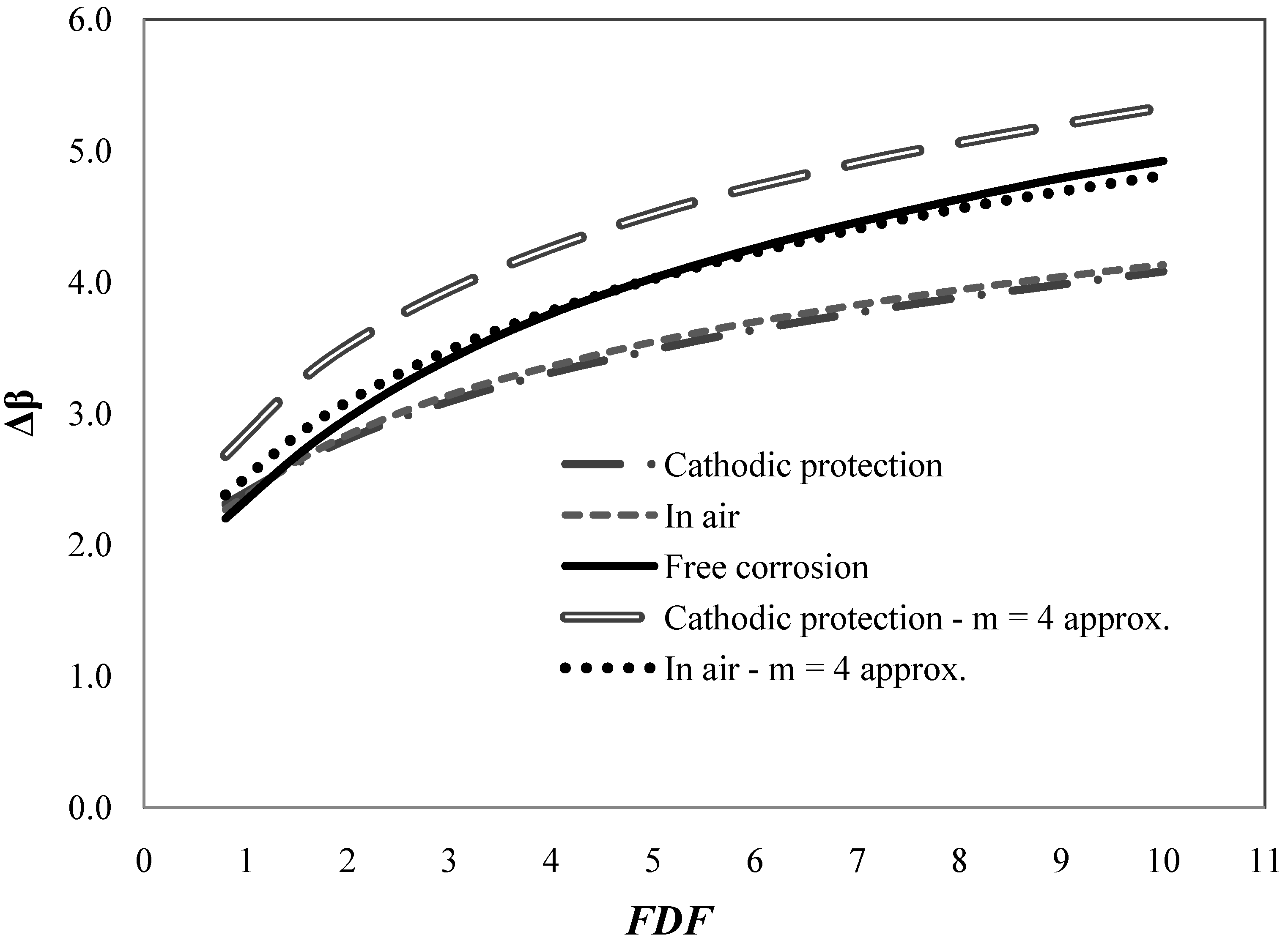
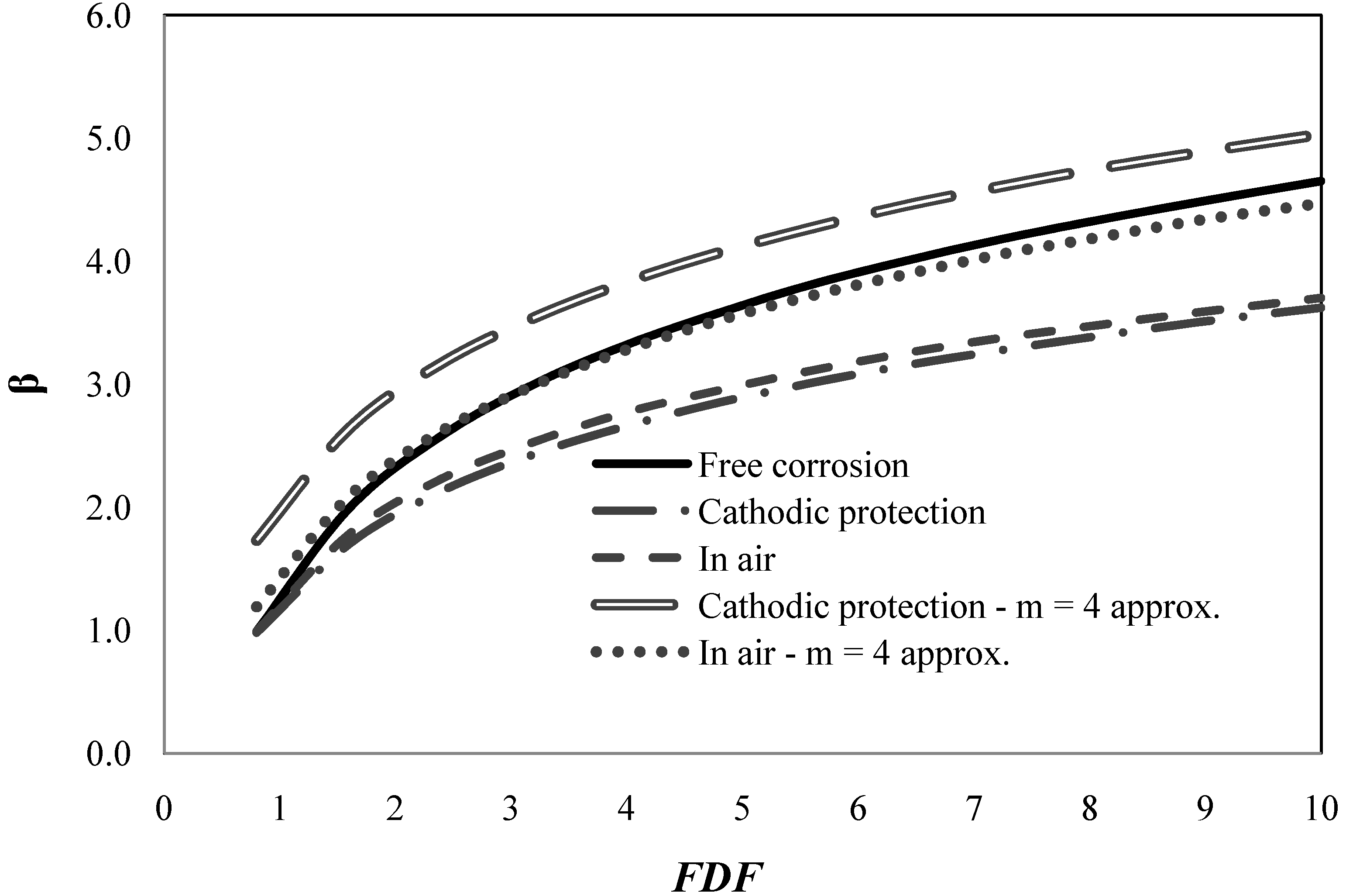
The results shows that required FDF values determined for cumulative reliability index equal to 2.5 and 3.1 and for an annual reliability index equal to 3.1 and 3.7 thus covering the range of reliability levels implicitly given in relevant standards. Figure 5 and Figure 6 show annual and cumulative reliability indices as function of FDF for T_L = 25 years and base values of coefficients of variation in Table 1. The reliability indices are shown for the three representative SN-curves mentioned in Section 2. It is seen that the bilinear SN-curves for “With cathodic protection” and “In air” results in almost the same reliability levels whereas the linear SN-curve for “Free corrosion” results in larger reliability indices, but at the same time also larger values of the design parameter z are obtained.

In practical design of wind turbine details for fatigue the bilinear SN-curve is often approximated by a linear SN-curve with slope m = 4 determined such that the linear SN-curve goes through the point where the bilinear SN-curve changes slope. Figure 5 and Figure 6 also show the reliability indices obtained using this conservative linear SN-curve for design and the bilinear SN-curve for reliability analysis. It is seen, as expected, that the reliability indices are significantly larger by this conservative approach, and therefore required FDF values could be lowered if this conservative approach is used.

Figure 5. Annual reliability index as function of FDF for T_L = 25 years and base values of coefficients of variation in Table 1.

Figure 5. Annual reliability index as function of FDF for T_L = 25 years and base values of coefficients of variation in Table 1.

Figure 6. Cumulative reliability index as function of FDF for life T_L = 25 years and base values of coefficients of variation in Table 1.

Figure 6. Cumulative reliability index as function of FDF for life T_L = 25 years and base values of coefficients of variation in Table 1.

5.1. Required FDF Values with No Inspections

In this section illustrative results are shown for required FDF values in the case where no inspections are performed. Table 6 and Table 7 show the required FDF values for minimum cumulative and annual reliability levels for the base case of the stochastic model in table 1 for the three representative SN-curves mentioned in section 2. The bilinear SN-curves for “With cathodic protection” and “In air” results in almost the same required FDF values whereas the linear SN-curve for “Free corrosion” results in smaller required FDF values.

Table 6. Required FDF values for minimum cumulative reliability level.

β	“With cathodic protection”	“In air”	“Free corrosion”
2.5	3.4	3.1	2.3
3.1	6.1	5.5	3.4

Table 6. Required FDF values for minimum cumulative reliability level.

β	“With cathodic protection”	“In air”	“Free corrosion”
2.5	3.4	3.1	2.3
3.1	6.1	5.5	3.4

Table 7. Required FDF values for minimum annual reliability level.

Δβ	“With cathodic protection”	“In air”	“Free corrosion”
3.1	3.0	2.9	2.3
3.7	6.5	6.1	3.9

Table 7. Required FDF values for minimum annual reliability level.

Δβ	“With cathodic protection”	“In air”	“Free corrosion”
3.1	3.0	2.9	2.3
3.7	6.5	6.1	3.9

Table 8, Table 9, Table 10, Table 11, Table 12 and Table 13 show the results of sensitivity analyses for different values of the coefficient of variations for X_SCF, X_W and Δ. It is seen as expected that relative changes of the COVs for X_SCF and X_W are more important than changes of COV for Δ.

Table 8. Required FDF values for SN-curve “With cathodic protection”. Sensitivity wrt COV [X_SCF] and minimum cumulative reliability level.

β\COV[XSCF]	0.05	0.10	0.15	0.20
2.5	2.7	3.4	4.8	7.3
3.1	4.5	6.1	9.3	>10

Table 8. Required FDF values for SN-curve “With cathodic protection”. Sensitivity wrt COV [X_SCF] and minimum cumulative reliability level.

β\COV[XSCF]	0.05	0.10	0.15	0.20
2.5	2.7	3.4	4.8	7.3
3.1	4.5	6.1	9.3	>10

Table 9. Required FDF values for SN-curve “With cathodic protection”. Sensitivity wrt COV[X_W] and minimum cumulative reliability level.

β\COV[XW]	0.10	0.15	0.20
2.5	3.4	4.8	7.3
3.1	6.1	9.3	>10

Table 9. Required FDF values for SN-curve “With cathodic protection”. Sensitivity wrt COV[X_W] and minimum cumulative reliability level.

β\COV[XW]	0.10	0.15	0.20
2.5	3.4	4.8	7.3
3.1	6.1	9.3	>10

Table 10. Required FDF values for SN-curve “With cathodic protection”. Sensitivity wrt COV[Δ] and minimum cumulative reliability level.

β\COV[Δ]	0.10	0.20	0.30
2.5	3.0	3.2	3.4
3.1	5.2	5.5	6.1

Table 10. Required FDF values for SN-curve “With cathodic protection”. Sensitivity wrt COV[Δ] and minimum cumulative reliability level.

β\COV[Δ]	0.10	0.20	0.30
2.5	3.0	3.2	3.4
3.1	5.2	5.5	6.1

Table 11. Required FDF values for SN-curve “With cathodic protection”. Sensitivity wrt COV[X_SCF] and minimum annual reliability level.

Δβ\COV[XSCF]	0.05	0.10	0.15	0.20
3.1	2.5	3.0	4.0	5.3
3.7	4.9	6.5	9.7	>10

Table 11. Required FDF values for SN-curve “With cathodic protection”. Sensitivity wrt COV[X_SCF] and minimum annual reliability level.

Δβ\COV[XSCF]	0.05	0.10	0.15	0.20
3.1	2.5	3.0	4.0	5.3
3.7	4.9	6.5	9.7	>10

Table 12. Required FDF values for SN-curve “With cathodic protection”. Sensitivity wrt COV[X_W] and minimum annual reliability level.

Δβ\COV[XW]	0.10	0.15	0.20
3.1	3.0	4.0	5.3
3.7	6.5	9.7	>10

Table 12. Required FDF values for SN-curve “With cathodic protection”. Sensitivity wrt COV[X_W] and minimum annual reliability level.

Δβ\COV[XW]	0.10	0.15	0.20
3.1	3.0	4.0	5.3
3.7	6.5	9.7	>10

Table 13. Required FDF values for SN-curve “With cathodic protection”. Sensitivity wrt COV[X_Δ] and minimum annual reliability level.

Δβ\COV[XΔ]	0.1	0.2	0.3
3.1	2.7	2.8	3.0
3.7	5.6	5.9	6.5

Table 13. Required FDF values for SN-curve “With cathodic protection”. Sensitivity wrt COV[X_Δ] and minimum annual reliability level.

Δβ\COV[XΔ]	0.1	0.2	0.3
3.1	2.7	2.8	3.0
3.7	5.6	5.9	6.5

Table 14 and Table 15 show the results of sensitivity analyses for different values of the coefficient of variations for COV[logK₁] and COV[logK₂]. It is seen as expected that relative changes of the COVs for logK₁ and logK₂ are less important than X_SCF and X_W but more important than changes of COV for Δ.

Table 14. Required FDF values for SN-curve “With cathodic protection”. Sensitivity wrt COV[logK₁]/COV[logK₂] and minimum cumulative reliability level.

β\COV[logK1]/COV[logK2]	0.10/0.15	0.15/0.20	0.20/0.25
2.5	4.1	3.7	3.4
3.1	6.7	6.3	6.1

Table 14. Required FDF values for SN-curve “With cathodic protection”. Sensitivity wrt COV[logK₁]/COV[logK₂] and minimum cumulative reliability level.

β\COV[logK1]/COV[logK2]	0.10/0.15	0.15/0.20	0.20/0.25
2.5	4.1	3.7	3.4
3.1	6.7	6.3	6.1

Table 15. Required FDF values for SN-curve “With cathodic protection”. Sensitivity wrt COV[logK₁]/COV[logK₂] and minimum annual reliability level.

β\COV[logK1]/COV[logK2]	0.10/0.15	0.15/0.20	0.20/0.25
2.5	3.8	3.4	3.0
3.1	7.3	6.8	6.5

Table 15. Required FDF values for SN-curve “With cathodic protection”. Sensitivity wrt COV[logK₁]/COV[logK₂] and minimum annual reliability level.

β\COV[logK1]/COV[logK2]	0.10/0.15	0.15/0.20	0.20/0.25
2.5	3.8	3.4	3.0
3.1	7.3	6.8	6.5

Table 16 and Table 17 show the results of if the linearized model for the stress ranges in Figure 1 is used. It is seen the changes in required FDF values is quite small indicating that the shape of the stress distribution is less important. However, the total number of stress cycles is important since it determines how much of the fatigue damage is related to the two slopes of the bilinear SN-curve. For linear SN-curves the shape of the stress distribution is without importance.

Table 16. Required FDF values using a linearized model for stress ranges for minimum cumulative reliability level. Base case values in ( ).

β	“With cathodic protection”	“In air”	“Free corrosion”
2.5	3.3 (3.4)	2.9 (3.1)	2.3 (2.3)
3.1	5.9 (6.1)	5.1 (5.5)	3.4 (3.4)

Table 16. Required FDF values using a linearized model for stress ranges for minimum cumulative reliability level. Base case values in ( ).

β	“With cathodic protection”	“In air”	“Free corrosion”
2.5	3.3 (3.4)	2.9 (3.1)	2.3 (2.3)
3.1	5.9 (6.1)	5.1 (5.5)	3.4 (3.4)

Table 17. Required FDF values using a linearized model for stress ranges for minimum annual reliability level. Base case values in ( ).

Δβ	“With cathodic protection”	“In air”	“Free corrosion”
3.1	3.0 (3.0)	2.7 (2.9)	2.3 (2.3)
3.7	6.4 (6.5)	5.6 (6.1)	3.9 (3.9)

Table 17. Required FDF values using a linearized model for stress ranges for minimum annual reliability level. Base case values in ( ).

Δβ	“With cathodic protection”	“In air”	“Free corrosion”
3.1	3.0 (3.0)	2.7 (2.9)	2.3 (2.3)
3.7	6.4 (6.5)	5.6 (6.1)	3.9 (3.9)

5.2. Required FDF Values with Inspections

Table 18 and Table 19 show the required FDF values if equidistant inspections are performed. Two types of inspections are considered:

• Inspection with Eddy Current, see POD-curve in Table 5
• Visual inspection with an exponential POD-curve with expected value of the smallest detectable cracks lengths equal to 50 mm.

Further, it is assumed that the crack length, c to crack depth, a ratio in (14) is five, i.e., $f\left(\frac{a}{T}\right)=10.$ The results show that significant reductions in required FDF values can be obtained if inspections are performed.

Table 18. Required FDF values for minimum cumulative reliability level. SN-curve: “With cathodic protection”. Close visual inspection.

β/number of inspections	0	1	2	4	10
2.5	3.4	2.7	2.3	1.3	1
3.1	6.1	5.0	4.1	2.8	1

Table 18. Required FDF values for minimum cumulative reliability level. SN-curve: “With cathodic protection”. Close visual inspection.

β/number of inspections	0	1	2	4	10
2.5	3.4	2.7	2.3	1.3	1
3.1	6.1	5.0	4.1	2.8	1

Table 19. Required FDF values for minimum cumulative reliability level. SN-curve: “With cathodic protection”. Inspections with the Eddy Current technique.

β/number of inspections	0	1	2	4	10
2.5	3.4	3.0	2.7	2.3	1
3.1	6.1	5.3	5.0	3.6	1.3

Table 19. Required FDF values for minimum cumulative reliability level. SN-curve: “With cathodic protection”. Inspections with the Eddy Current technique.

β/number of inspections	0	1	2	4	10
2.5	3.4	3.0	2.7	2.3	1
3.1	6.1	5.3	5.0	3.6	1.3

6. Conclusions

For offshore wind turbines lower fatigue safety factors can be expected compared to those required for offshore oil & gas platforms since the consequences of failure are in general lower. In this paper a reliability based approach is used to assess the fatigue safety factors required for welded details in support structures for offshore wind turbines. The expected future development within offshore wind energy will require more wind turbines placed at deeper water implying more focus new innovations within support structures and on optimizing the material consumptions including design for the fatigue failure mode.

In the reliability-based approach probabilistic models have been developed partially based on experience from offshore oil & gas structures, where design and limit state equations are established for fatigue failure. The strength and load uncertainties are described by stochastic variables. SN and fracture mechanics approaches are considered for to model the fatigue life. Further, both linear and bi-linear SN-curves are formulated and various approximations are investigated. The acceptable reliability level for fatigue failure of OWT’s is discussed based on recommendations for fatigue design factors/safety factors in various standards related to offshore wind turbines. It seems that an cumulative reliability index between 2.5 and 3.1 are reasonable for fatigue design of welded details.

Fatigue design factors (FDF) are calibrated to this reliability level using representative models for uncertainties and fatigue loads. The results show that in general the FDFs should be increased compared to the values currently recommended in standards. However, it is also seen that the FDFs depend highly on the level of uncertainty of the assessment of the loads and the stress concentration factors. If these uncertainties are decreased then much smaller FDFs are obtained. The influence of modelling the stress ranges is investigated with the result that the difference between the required FDF values for the basic stress range model and a linearized model is quite small (approx 2–4%). However, the total number of stress cycles is important since it determines how much of the fatigue damage is related to the two slopes of the bilinear SN-curve.

For a practical design of wind turbine details a linear conservative SN-curve with slope equal to 4 was considered. As expected this conservative model implies a rather conservative design with a reliability level much higher than using the “correct” bilinear SN-curve.

Further, the influence of inspections was considered in order to extend and maintain a given target safety level. The results show that significant reductions in required FDF values can be obtained if inspections are performed.

The results presented in this paper describe the basic approach that can be used for assessment of the required reliability level and fatigue design factors for support structures for offshore wind turbines. Future work should include also the effect of wakes in wind farms increasing the turbulence level and thus the fatigue loads significantly. Also design for fatigue of details made in various types of concrete could be expected to be important for future innovative offshore wind turbine support structures.