A High Performance Real-Time Simulator for Controllers Hardware-in-the-Loop Testing

Abstract

This paper presents a high performance real-time simulator for power electronic systems applications and primarily intended for controller hardware-in-the-loop (CHIL) testing. The novelty of the proposed simulator resides in the massively parallel hardware architecture that efficiently exploits fine-grained parallelism without imposing severe communication overhead time that can limit the performance. The simulator enables the use of a nanosecond range simulation timestep to simulate power electronic systems. Through the use of this nanosecond range simulation timestep, the simulator minimizes the error arising from the intersimulation timestep switching phenomenon associated with CHIL. The proposed hardware architecture is realized based on the FPGA technology. The simulator is tested and its CHIL capability verified based on the closed-loop testing of a robust multivariable servomechanism controller for autonomous operation of a distributed generation unit.

1. Introduction

Microgrids and smart grids are the new concepts which have been brought about due to high penetration of renewable energy systems, distributed generation (DG) units, and storage systems. The environmental issues and economical, social, and political interests make the role of microgrid even more important. Nowadays, the use of DG units and microgrid systems is mainly limited to their operation in the grid-connected mode. In the grid-connected mode, a microgrid including its loads and DG units is connected to the main grid at the point of common coupling (PCC). In this case, the main grid provides fixed voltage and frequency for the microgrid and each DG unit regulates its power components based on the conventional dq-current control strategy. The set points for the dq-current controllers are determined such that the maximum power generated by the distributed energy sources is achieved.

Autonomous (islanded) operation of a microgrid, however, is not as straightforward as its operation in the grid-connected mode, i.e., control and power management of an islanded microgrid is very difficult due to the stochastic nature of the renewable energy sources that act as the prime movers for the DG units. An islanded microgrid is a low inertia system whose dynamics highly vary due to the load perturbations. Therefore, the reliable and robust operation of a microgrid in the autonomous mode requires sophisticated control strategies which should guarantee desirable performance criteria and secure operation in a wide range of operating conditions.

Time-domain simulation has a vital role in the design, development, implementation and verification cycles of controllers platforms. During early design stages, offline simulation softwares are used for verification and performance evaluation of the design concepts. Thereafter, the implementation stage begins where the control algorithm is realized on a physical platform. A hardware-in-the-loop (HIL) arrangement of a physical controller platform, in association with a real-time simulator, is needed to safely and thoroughly verify the design integrity and evaluate its functions and performance [1,2,3,4]. This type of HIL testing, involving the exchange of waveforms between the simulator and the controller platform at the signal level with no real power exchange, is called controller hardware-in-the-loop (CHIL) testing.

The existing real-time simulators utilize parallel processing, where multiprocessors, either General Purpose Processors (GPP) or Digital Signal Processors (DSP), or computer clusters are utilized [5,6,7,8,9,10,11,12], to achieve the required real-time simulation performance. The system to be simulated is divided into zones, and the mathematical model of each zone is assigned to a given processor. A master processor (i) controls the communication and (ii) maintains synchronism among the other processors. In such paradigm, the minimum simulation timestep is dictated by the speed and number of processors, the synchronization and communication overhead time among the processors, and the efficiency of the software code.

However, existing real-time simulators have limitations on (i) the minimum timestep size which is roughly between 10 and 80 μs, (ii) the frequency bandwidth of the simulation results [13] which is approximately up to 10 kHz, and (iii) the accuracy of the adopted models. The relatively large simulation timestep of existing simulators hinders the simulation of high-frequency converters and generally compromises the accuracy of HIL testing since switching events imposed by the controller within one timestep cannot be accounted for by the simulator until the subsequent timestep. Moreover, increasing the frequency bandwidth of the simulation results inherently requires not only the use of a smaller simulation timestep but also the use of more accurate models. However, improving the accuracy based on adopting more elaborate models increases the computational time and violation to real-time constraints occurs. These conflicting requirements necessitate a compromise between accuracy and computation performance for real-time simulators [14,15].

The limitations of existing real-time simulators are the main motivation behind the development of the FPGA-based real-time simulator presented in this paper. This paper builds on the parallel implementation methodology of [16,17,18] and realizes a high performance FPGA-based real-time simulator for CHIL testing. The novelty of the proposed simulator resides in the massively parallel hardware architecture that is “tailored" to the solution of the mathematical model of the system under consideration. Thus, the hardware is not fixed but changes, depending on the system model, to maximize the computational performance. Moreover, this parallel hardware architecture efficiently exploits fine-grained parallelism without imposing sever communication and synchronization overhead times that can limit the performance. This simulator also provides the inherent capability to relax the accuracy and bandwidth limits of the existing real-time simulators.

The rest of this paper is organized as follows. Section II elaborates on the interfacing issues associated with CHIL testing. Section III presents the architecture of the proposed FPGA-based real-time simulator. Section IV introduces the proposed techniques to interface the external control/protection platform with the simulator and the different options for monitoring of the waveforms generated inside the simulator. Sections V and VI, through a case study, provide validation and evaluation of the performance of the developed simulator. Conclusions are stated in Section VII.

2. CHIL Interfacing Issues

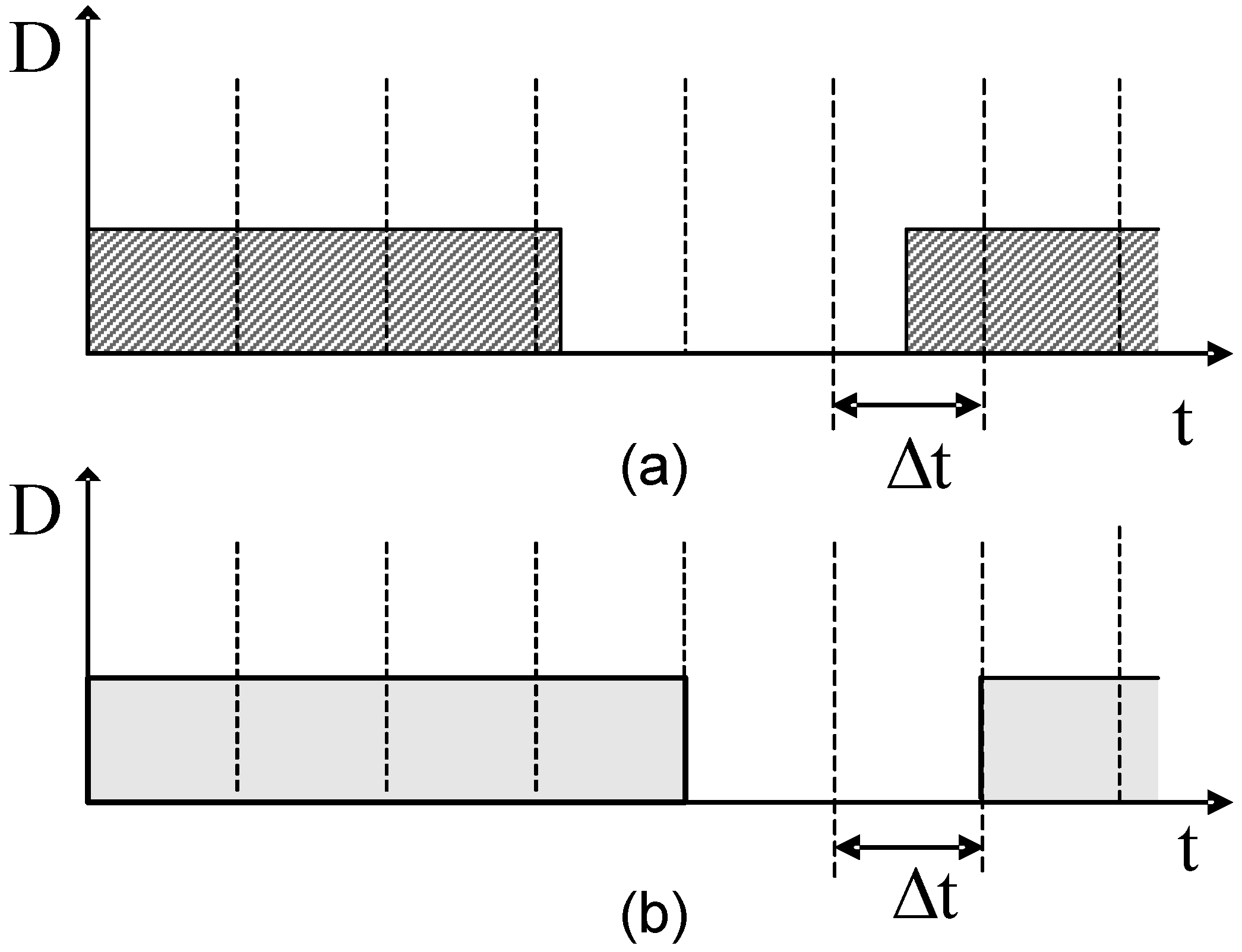
CHIL testing involves real-time data exchange between the real-time simulator and the controller platform under test. To ensure a deterministic operating behavior and to reduce the computational complexity, the real-time digital simulator adopts a fixed simulation timestep. The simulator reads the gating signals issued by the controller and updates the states of the power electronic switches only at the beginning of a simulation time instant. However, due to the discrete nature and the inherent variability in the pulse width of the PWM outputs of the controller, it is unlikely that the switching events coincide with the simulation time instances on the simulator time-grid, i.e., switching events are imposed between two simulation time instances. This intersimulation timestep switching (ITS) phenomenon is not limited to just one switching event between two simulation time instances. Multiple switching events are also possible. The number of switching events depends on (i) the ratio between the inverse of the simulation timestep and the switching frequency of the PWM signal, and (ii) the number of switches in the systems.

The ITS introduces errors and jitter to the simulation results as the PWM input considered by the simulator is different from the actual PWM generated by the controller (Figure 1). The percentage error due to ITS is a function of the simulation timestep of the simulator and the switching frequency of the controller. Practically, if the simulation timestep is hundred times less than the switching period, the error due to the ITS events can be neglected [16,19].

The simulation timestep of the existing real-time simulators are not sufficiently small to eliminate the error due to ITS. Thus corrective measures to account for the errors due to ITS events are needed. These corrective measures utilize time stamping techniques and interpolations/extrapolations to (i) register the exact switching time instance, (ii) determine the system variables at the switching time instant, and (iii) resynchronize the simulator output with the simulation time grid [19,20,21,22,23,24].

Figure 1. (a) Actual PWM generated by the controller; (b) PWM input considered by the simulator.

Figure 1. (a) Actual PWM generated by the controller; (b) PWM input considered by the simulator.

It should be noted that the corrective measures have limitations. First, they do not produce correct outputs at the timestep in which the ITS occurred; rather they only help to prevent the simulator from commencing the calculations in the next timestep based on incorrect values of the system variables. The produced outputs, at the timestep in which the ITS occurred, belong to one of the following two categories:

• The original incorrect values calculated without accounting for the switching event [23]: This is the case when the corrective algorithm is initiated at the next timestep since the real-time operation does not permit going back in time to correct the system variables.
• The interpolated values at the switching instant [22]: This is the case when the corrective algorithm is initiated before issuing the outputs.

Addressing multiple switching events, based on these corrective measures [25], result in a significant computational burden since multiple interpolations/extrapolations within each simulation timestep are required which in turn can limit or even violate real-time calculation requirements [26].

In this work, the proposed FPGA-based real-time simulator utilizes a massively parallel, customized, hardware architecture that is specifically designed to allow the real-time simulation of power electronic systems with timesteps significantly smaller than those of existing real-time simulators, e.g., tens to few hundreds of nanoseconds. Thus, it eliminates the need for corrective measures, to account for the error due to single and multiple ITS events, without compromising the accuracy or the numerical stability of the simulation.

3. FPGA-Based Real-Time Simulator Architecture

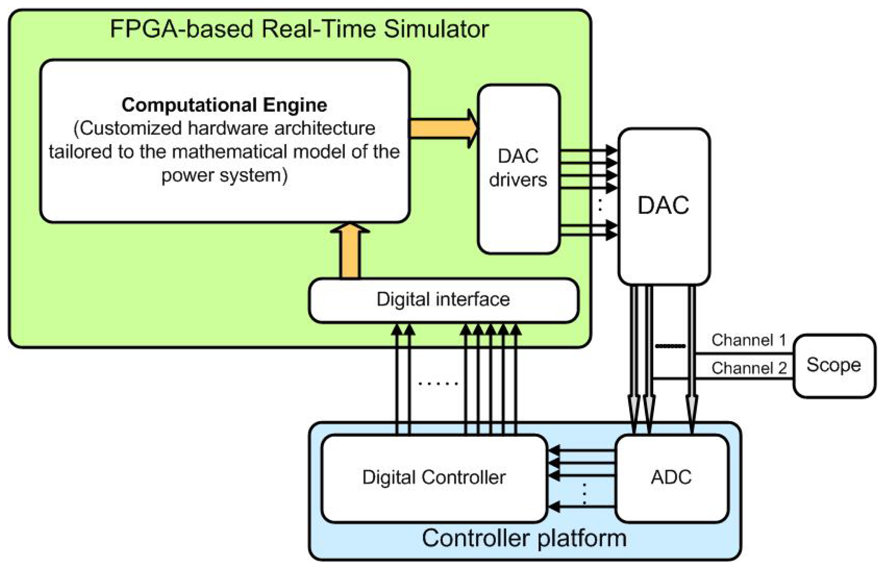
Figure 2 shows a schematic diagram of the FPGA-based real-time simulator. The core of the simulator is the computational engine. The computational engine is designed to provide the following main operational characteristics:

• speed, i.e., a computation time in the range of tens to few hundreds of nanoseconds, and
• scalability, i.e., can be expanded to accommodate larger systems without impacting the simulation timestep.

Figure 2. Schematic of the FPGA-based real-time simulator in HIL testing arrangement.

Figure 2. Schematic of the FPGA-based real-time simulator in HIL testing arrangement.

The design philosophy of the computational engine, to fulfill the aforementioned design requirements, is to:

• exploit all possible levels of parallelism inherent to the solution algorithm of the system model, and
• design a customized hardware architecture that closely maps both the solution algorithm and dataflow.

The solution algorithm adopted in this work is a variation of the generalized algorithm of [27,28]. The main difference is that the backward Euler method instead of the trapezoidal method is used. The backward Euler method provides damping to numerical oscillations that arise due to discontinuities, e.g., switchings, unlike the trapezoidal method which introduces sustained numerical oscillations due to switching events [29].

The solution algorithm is based on representing each circuit component by its companion circuit model. As such, the original system is transformed into a system of resistive elements and current sources. Nodal analysis is then used to solve for the node voltages at each timestep [27,30]. The nodal equation is given by

$$Yv\left(t\right)=i\left(t\right)-I$$

(1)

where Y is the nodal admittance matrix, $v\left(t\right)$ is the vector of the node voltages, $i\left(t\right)$ is the vector of current sources, and I is the vector of history current sources. Typically, the value of a given history current source h is computed by

$$h\left(t\right)=\gamma v\left(t\right)+\kappa h(t-\Delta t)$$

(2)

where γ and κ are constants and calculated from the components parameters and the timestep.

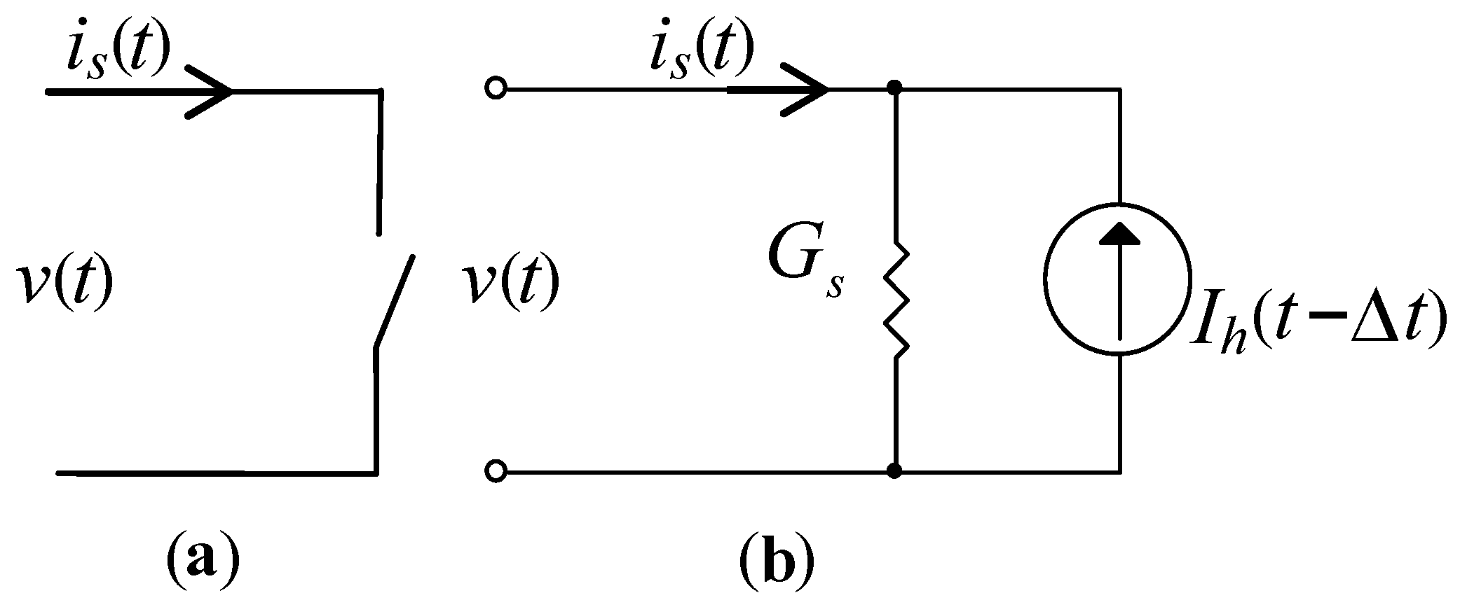
It has to be noted that, for a fixed simulation timestep, the right hand side of Equation (1) is updated in each simulation timestep, whereas the nodal admittance matrix Y remains constant. The associated discrete circuit (ADC) modeling approach extend the companion modeling approach to power electronic switches. The ADC approach represents a power electronic switch with a current source in parallel with a conductance $G_S$ (Figure 3) [31,32,33,34,35]. In this approach, the conductance $G_S$ is fixed irrespective of the switch ON/OFF state. The switch ON/OFF state is only accounted for by the value of the shunt current source. Thus, the ADC approach maintains the admittance matrix constant irrespective of the ON/OFF state of each switch [31,32].

Figure 3. (a) Switch; (b) ADC switch model.

Figure 3. (a) Switch; (b) ADC switch model.

It is clear from the aforementioned discussion that the overall mathematical model of the system boils down to two sets of equations:

• the nodal equation of Equation (1). This is a set of M linear equations, where M is the number of nodes of the system, and
• the set of history current sources equations. This is a set of N equations in the form of Equation (2), where N is the number of history current sources.

The solution of the nodal Equation (1) is essentially the solution of the classical linear problem $Ax=b$. Since the entries of the admittance matrix of the system are kept unchanged, the solution of $Ax=b$ can be obtained by pre-calculating the inverse of A at the software level, i.e., before hardware implementation on the FPGA. Thus, there is no need to perform matrix inversions on the FPGA to solve Equation (1) and the solution of Equation (1) is converted to the matrix-vector multiplication of Equation (3)

$$x=A^{-1}b$$

(3)

Mathematically, a matrix-vector multiplication is the dot-product of each row of the multiplier matrix by the multiplicand vector. This is mathematically expressed in the form of a sum of product (SOP)

$$x\left(i\right)=\sum _{j=1}^M{A}^{-1}(i,j)b\left(j\right)$$

(4)

where $i=1,2,\dots ,M$.

The M SOP equations of Equation (4) are independent from one another and therefore they can be solved in parallel. This constitutes one level of parallelism which is at the equations level. The multiplication operations involved in the computation of the SOP of Equation (4) are independent and can be carried out in parallel. This constitutes a second level of parallelism which is at the level of “primitive operations".

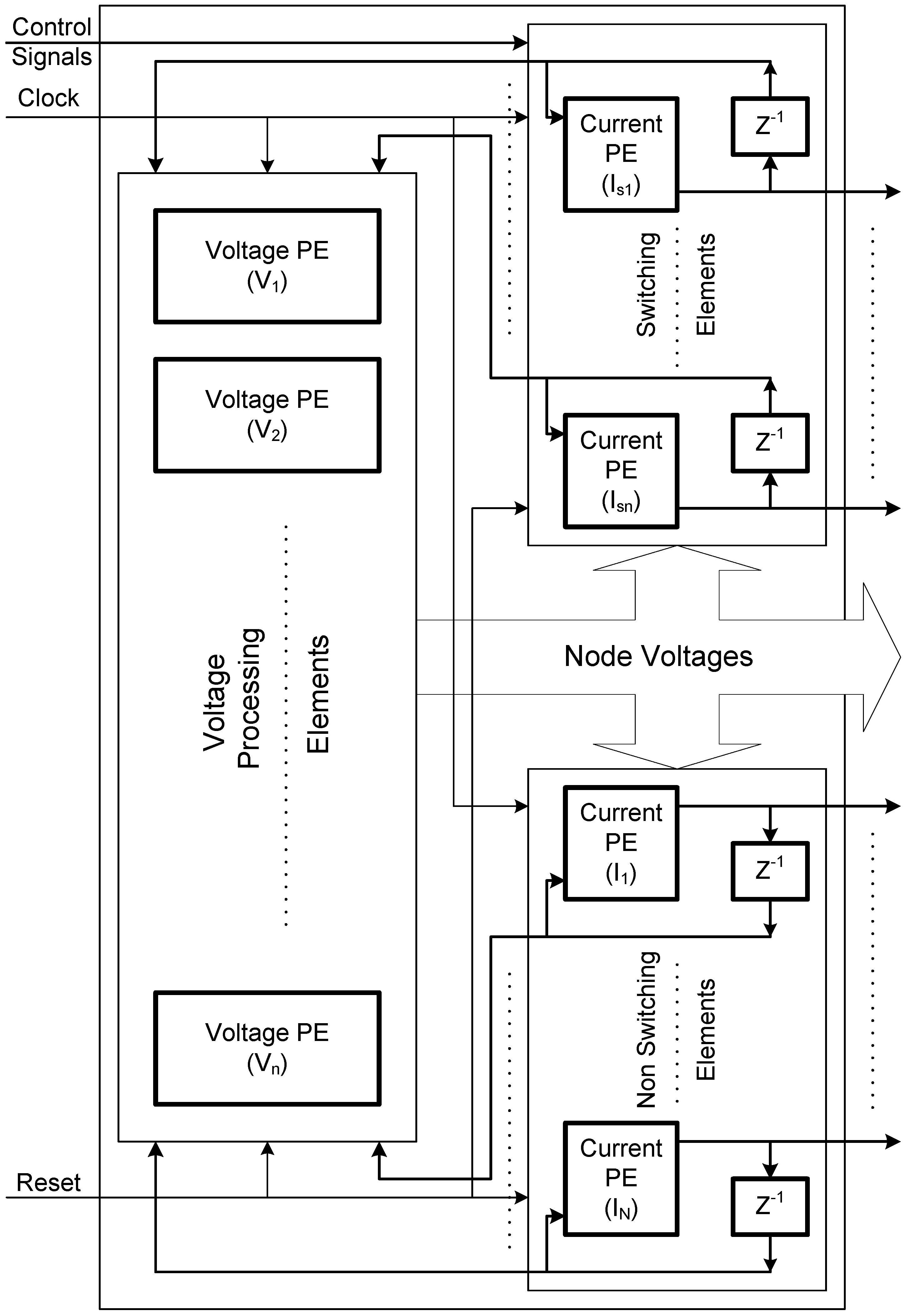
The computational engine is designed such that it has a massively parallel hardware architecture that exploits these two levels of parallelism. Figure 4 shows the functional diagram of the proposed hardware architecture implemented inside the FPGA-based real-time simulator. The module has three main building blocks:

• the first building block is responsible for calculating the node voltages, and
• the second and third building blocks are responsible for updating the history current sources associated with switching and non-switching elements, respectively.

Figure 4. Functional diagram of the computational engine.

Figure 4. Functional diagram of the computational engine.

It has to be noted that in this scheme the matrix-vector multiplication of Equation (3) is actually performed based on utilizing $n^2$ parallel multipliers. As shown in Figure 4, the design has n parallel voltage processing elements. Each processing element is responsible for evaluating the voltage at a given node. Within each processing element, there are n parallel multipliers and an adder tree.

The history current sources are updated in parallel in a similar manner. Each history current source equation is assigned to a dedicated current processing element. Within each processing element, there are a number of parallel multipliers and an adder tree. Moreover, a current processing element for switching devices has additional control circuitry to determine the ON/OFF states of the switching element based on internal variable, i.e., voltage across the switch and/or current through it, or external control signals if it is controllable.

In massively parallel architectures, communication and synchronization among processing elements play a vital role in determining the overall system performance. Improper communication and synchronization schemes result in large overhead time that can severely limit the overall system performance. In this work, to minimize the communication and synchronization overhead times, a unidirectional point-to-point static interconnection network is implemented such that the data can be transferred directly from the outputs of one processing element to the inputs of another one. The whole design, i.e., the processing elements and the interconnection network, is operated in a synchronous mode with a global clock controlling both the computations and the dataflow.

4. Interfacing with External Control Platforms

HIL testing involves data exchange between the real-time simulator and the controller platform. The inputs to the controller platform are usually analog in nature since in real-life operation these inputs are voltage and current measurements from the actual power system. On the other hand the outputs from the controller platform—the PWM gating signals—are inherently digital. Thus, the gating signals are transferred directly from the Controller platform to the simulator in digital. The number of digital inputs to the simulator is equal to the number of control signals, which is dictated by the number of switching devices present in the power system being simulated.

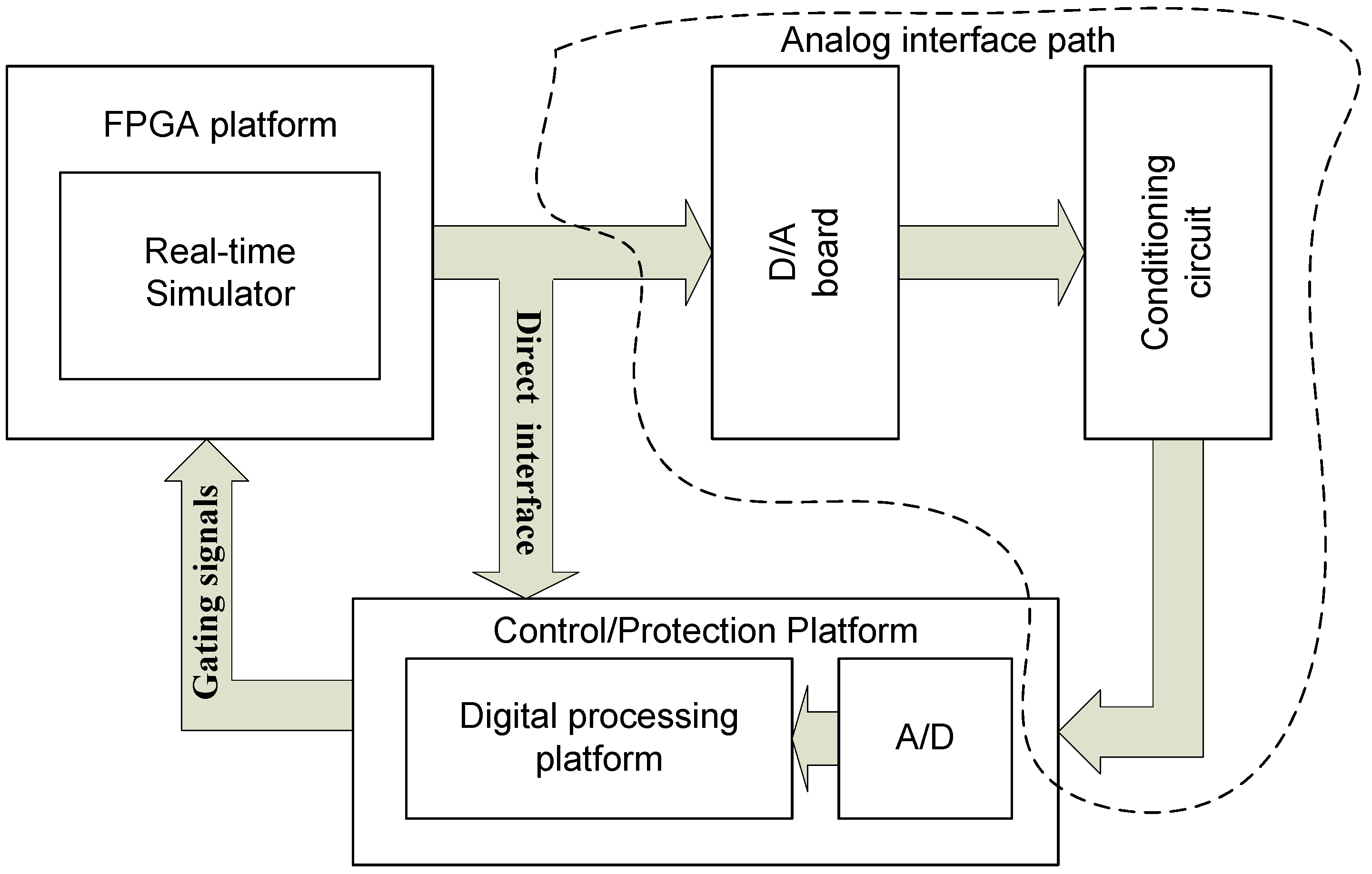
The FPGA-based real-time simulator provides two options for transferring the real-time simulator outputs to the external Controller Platform; either via (i) an analog interface, which utilizes digital-to-analog converters (DAC) to generate analog signals corresponding to the simulated voltages and currents, or via (ii) a direct digital interface (Figure 5).

The analog interface is useful when there is no access available to the Control/Protection digital signal processing platform except through its own analog-to-digital converters (ADC), or if it is required to evaluate the performance of the complete Control/Protection platform including its data converter systems. Moreover, the presence of the analog interface along with amplifiers enables the use of the simulator to operate in a power-hardware-in-the-loop (PHIL) configuration. In this configuration, physical power system components, e.g., machines, power electronic converters, etc., can be interfaced directly to the simulator [36,37,38]. In this work, DAC boards based on the Linear Technologies 16-bits parallel input LTC1668 DAC are developed to be used with the FPGA-based real-time simulator. The main advantage of this DAC unit is its very small settling time of approximately 20 ns, i.e., the overhead time due to the digital to analog conversion process is limited.

Figure 5. Simulator/controller interface options.

Figure 5. Simulator/controller interface options.

The direct digital interface enable the direct transmission of the digital signals, corresponding to the simulated voltages and currents, to the Control/Protection Platform. This scheme is useful in verifying the implementation of the control/protection algorithm on the Control/Protection digital signal processing platform during the development stage.

Regardless of the output format from the simulator, i.e., digital or analog, the outputs have to be synchronized with the simulator time grid. In this work, the simulator outputs are updated based on the rising edge of the simulator clock.

5. Case Study: HIL Testing of a Robust Controller for Autonomous Operation of a Distributed Generation Unit

The main objective of this test case is to demonstrate the capability of the FPGA-based simulator to operate in a hardware-in-the-loop configuration. The real-time simulator is interfaced with an external controller and the complete setup, i.e., the simulator and the controller, is operated in closed loop.

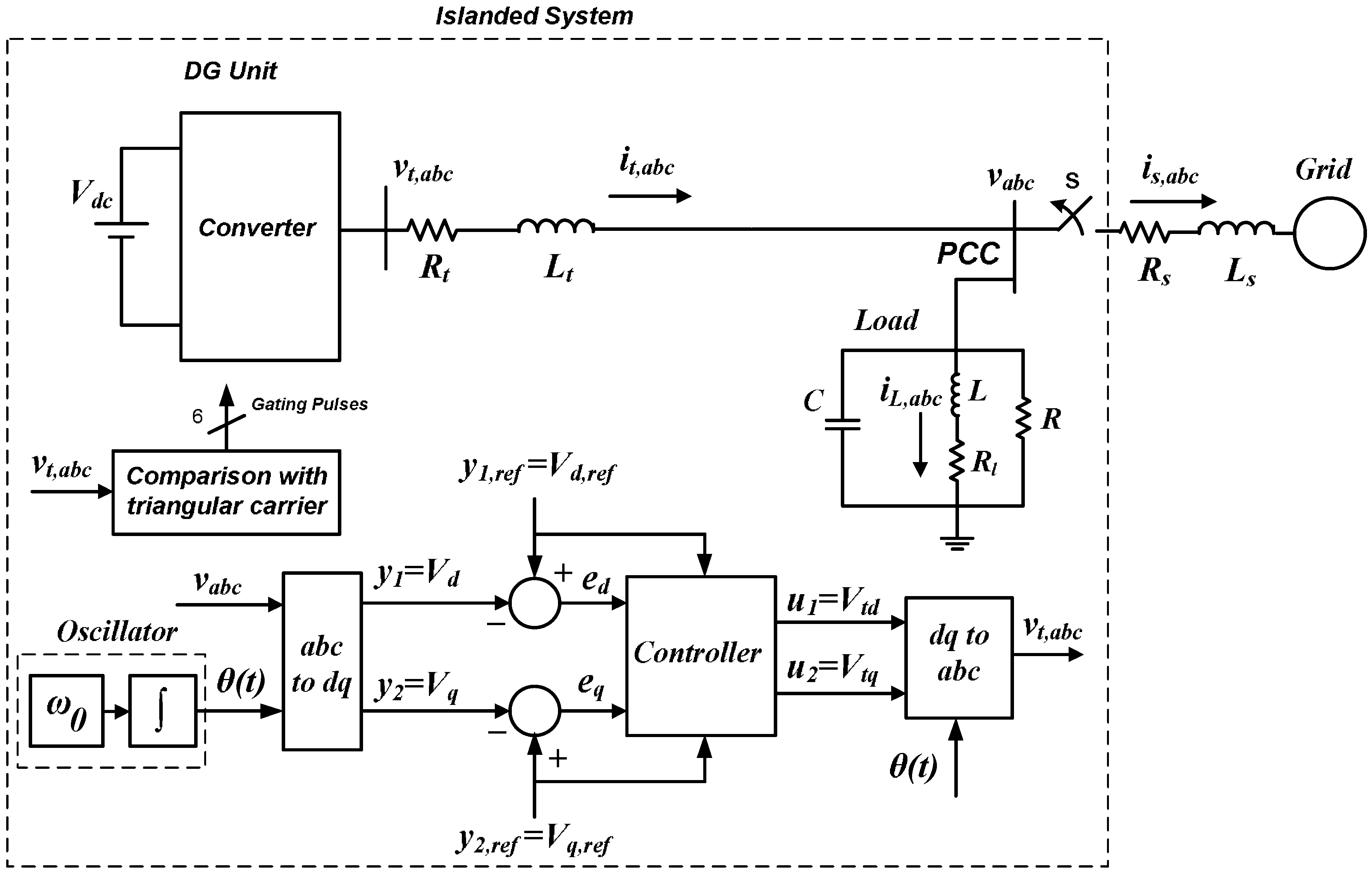
Figure 6 shows the single line diagram of the DG system under consideration. The DG unit is composed of a two-level voltage-sourced converter (VSC), a DC voltage source, and a series filter. The local load is a three-phase parallel RLC circuit. The system parameters are given in Table 1.

5.1. System Model for Controller Design

The state-space representation of the islanded system of Figure 6, in the abc-frame, is

$$\left\{\begin{array}{cc}\hfill i_{t,abc}& ={\displaystyle \frac{1}{R}}{v}_{abc}+i_{L,abc}+C{\displaystyle \frac{d{v}_{abc}}{dt}}\hfill \\ \hfill v_{t,abc}& =L_t{\displaystyle \frac{d{i}_{t,abc}}{dt}}+R_t{i}_{t,abc}+v_{abc}\hfill \\ \hfill v_{abc}& =L{\displaystyle \frac{d{i}_{L,abc}}{dt}}+R_l{i}_{L,abc}\hfill \end{array}\right.$$

(5)

where $v_{t,abc}$, $i_{t,abc}$, $i_{L,abc}$, and $v_{abc}$ are $3\times 1$ vectors comprising the individual phase quantities of Figure 6.

Figure 6. Schematic diagram of the islanded system and its controller.

Figure 6. Schematic diagram of the islanded system and its controller.

Table 1. Case I: System parameters.

Vdc	RTL	LTL	R	C	L	RL
46 kV	0.8 Ω	158 mH	76 Ω	62 μF	111.9 mH	0.1 Ω

Table 1. Case I: System parameters.

Vdc	RTL	LTL	R	C	L	RL
46 kV	0.8 Ω	158 mH	76 Ω	62 μF	111.9 mH	0.1 Ω

The state-space model in the abc frame, i.e., Equation (5), is then transformed to a rotating reference frame [39]. The state-space model in the dq frame is thus given by:

$$\left\{\begin{array}{cc}\hfill \dot{x}\left(t\right)& =Ax\left(t\right)+Bu\left(t\right)\hfill \\ \hfill y\left(t\right)& =C_{m}x\left(t\right)\hfill \\ \hfill e\left(t\right)& =y\left(t\right)-y_{ref}\left(t\right)\hfill \end{array}\right.$$

(6)

where $x={\left[V_d{V}_q{I}_{td}{I}_{tq}{I}_{Ld}{I}_{Lq}\right]}^{\prime }$ is the vector of state variables, $u={\left[V_{td}{V}_{tq}\right]}^{\prime }$ is the input vector, $y={\left[V_d{V}_q\right]}^{\prime }$ is the output vector, $y_{ref}$ is the reference input, e is the error in the system, and A, B, $C_m$ are constant matrices [40]. The open-loop system (6) includes two control inputs, i.e., $m=2$, and two outputs to be controlled, i.e., $r=2$. Reference signal $y_{ref}$ belongs to the class of step signals.

5.2. Robust Servomechanism Controller

The robust servomechanism controller of [40] is employed to regulate the voltage of the islanded system, whereas an internal oscillator is used to set the frequency of the islanded system (Figure 6). The frequency of the internal oscillator is set at the system nominal frequency.

As proposed on [40], a robust controller is designed to solve the robust servomechanism problem (RSP) [41,42,43,44,45] for the case of constant signals, in conjunction with the new proposed robustness constraint in [46]. Since the plant is minimum phase [40], in principle, we can achieve “perfect control” [43] for the system [40].

Controller Design Procedure: Consider the following “cheap control” performance index [44]:

$$J_{ϵ}={\int }_0^{\infty }(e^{\prime }e+ϵ{\nu }^{\prime }\nu )d\tau ,ϵ>0$$

(7)

that should be minimized for the system

$$\begin{array}{cc}\hfill \dot{\tilde{x}}& =\left[\begin{array}{cc}A& 0\\ {\mathcal{B}}_c{C}_m& {\mathcal{A}}_c\end{array}\right]\tilde{x}+\left[\begin{array}{c}B\\ 0\end{array}\right]\nu \hfill \\ \hfill e& =\left[\begin{array}{cc}0& {\mathcal{C}}_c\end{array}\right]\tilde{x}\hfill \end{array}$$

(8)

where $\tilde{x}={\left[x^{\prime }{\eta }^{\prime }\right]}^{\prime }$, e is the error in the system, and

$$\dot{\eta }={\mathcal{A}}_c\eta +{\mathcal{B}}_{c}e$$

(9)

is the servo-compensator [41] for the system, where

$$\begin{array}{cccc}\hfill {\mathcal{A}}_c& ={\left[\begin{array}{ccc}0& I& 0\\ 0& 0& I\\ 0& -{{\omega }^{*}}^{2}I& 0\end{array}\right]}_{6\times 6},\hfill & \hfill {\mathcal{B}}_c& ={\left[\begin{array}{c}0\\ 0\\ I\end{array}\right]}_{6\times 2}\hfill \\ \hfill {\mathcal{C}}_c& ={\left[\begin{array}{ccc}I& 0& 0\end{array}\right]}_{2\times 6},\hfill & \hfill {\omega }^{*}& =12440.7\hfill \end{array}$$

(10)

${\omega }^{*}=12440.7$ is the frequency of switching harmonics generated by the VSC. Since Equation (8) is stabilizable and detectable, the optimal controller which minimizes Equation (7), subject to Equation (8), is a stabilizing controller. In this case, a standard observer [43] can be used to implement the resultant optimal state feedback controller obtained in minimizing Equation (7) as given by:

$$\nu =K_{0}x+K_1\eta$$

(11)

where $K_0$ and $K_1$ are constant gain matrices [43]. In particular, as $ϵ\to 0$, zero channel interaction and arbitrary fast speed of response occurs, while no unbounded peaking occurs in the error response.

Assume now that the controller (11) is implemented by using an observer so that controller (11) becomes:

$$\begin{array}{cc}\hfill \left[\begin{array}{c}\dot{\xi }\\ \dot{\eta }\end{array}\right]& =\left[\begin{array}{cc}A-\Lambda C_m+B{K}_0& B{K}_1\\ 0& {\mathcal{A}}_c\end{array}\right]\left[\begin{array}{c}\xi \\ \eta \end{array}\right]+\left[\begin{array}{c}\Lambda \\ {\mathcal{B}}_c\end{array}\right]e\hfill \\ \hfill u& =\left[\begin{array}{cc}{K}_0& K_1\end{array}\right]\left[\begin{array}{c}\xi \\ \eta \end{array}\right]\hfill \end{array}$$

(12)

where $e=y-y_{ref}$ is the error in the system, and where Λ is the observer gain found so that $(A-\Lambda C_m)$ is stable, which can be represented as:

$$\begin{array}{cc}\hfill \dot{\beta }& ={\overline{\mathcal{A}}}_c\beta +{\overline{\mathcal{B}}}_c(y-y_{ref})\hfill \\ \hfill u& ={\overline{\mathcal{C}}}_c\beta \hfill \end{array}$$

(13)

Performing the design procedure of [40], the 12^th order strictly proper controller is obtained.

5.3. Hardware-in-the-Loop Setup

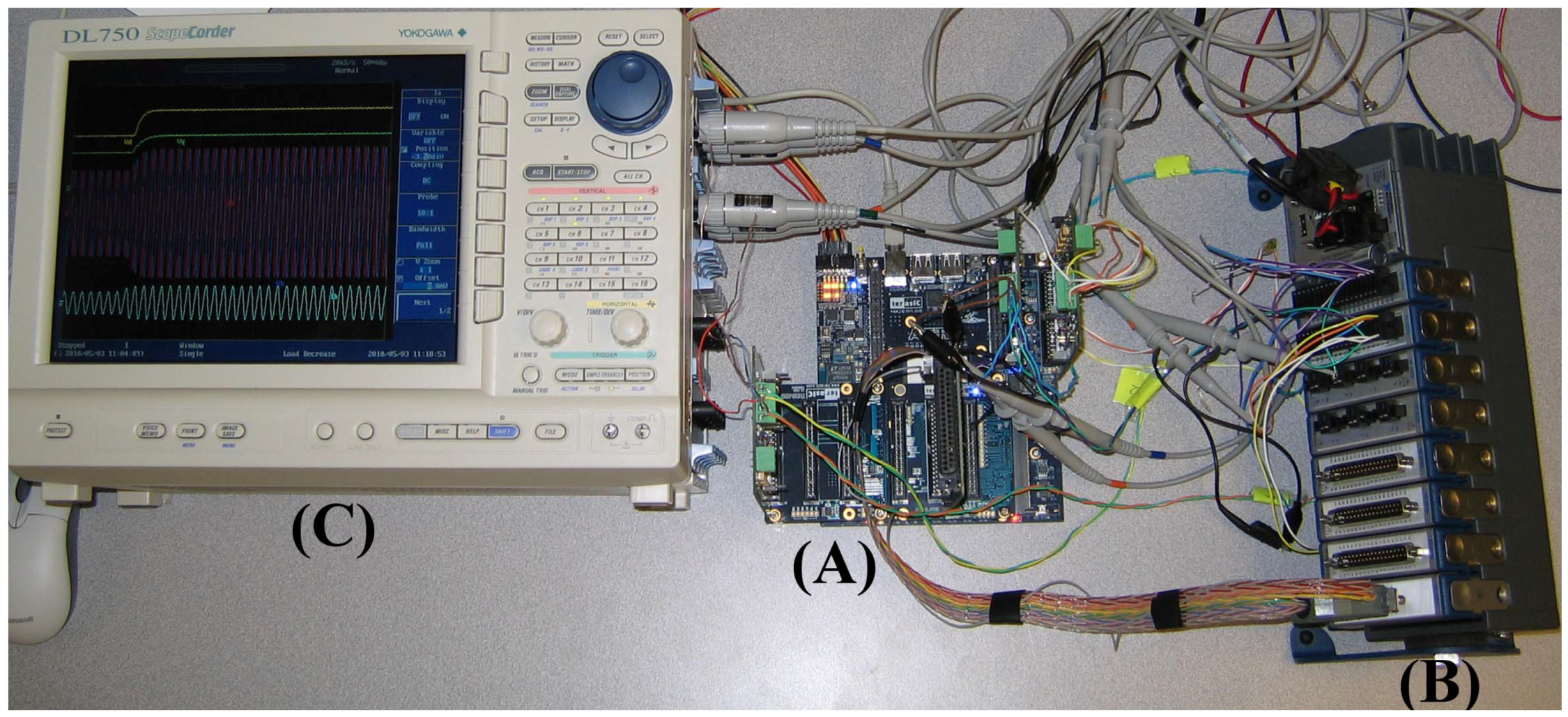
Figure 7 shows a photo of the FPGA-based real-time simulator in the HIL configuration. The real-time simulator is realized based on Altera’s DE3-150 Development and Education board [47], where the mathematical model of the converter system of Figure 6 is implemented inside the simulator Stratix III FPGA. The simulator operates in real-time with a fixed simulation timestep of 500 ns and the inputs to the simulator are 6 kHz PWM signals, i.e., the simulation timestep is approximately 340 times less than the switching period. Thus, there is no need for any corrective measures to account for the ITS or MITS as described in Section II. The VHDL language is used to describe the behavior of the designed hardware [48,49,50]. Altera Quartus II version 8 software tool is used for (i) design entry, (ii) design synthesis, (iii) fitting the design on the target FPGA, and (iv) programming the FPGA. The developed FPGA-based simulator is also very cost effective.

Figure 7. Photo of the experimental setup: (A) the FPGA-based real-time simulator; (B) the CRIO controller platform; and (C) the oscilloscope.

Figure 7. Photo of the experimental setup: (A) the FPGA-based real-time simulator; (B) the CRIO controller platform; and (C) the oscilloscope.

The controller and the sinusoidal pulse width modulator (SPWM) are implemented on the National Instrument CRIO platform comprised of an 800 MHz real-time PowerPC processor and a Virtex-5 LX110 FPGA. The control algorithm is expressed in C programming language and executed on the PowerPC processor. On the other hand, both the SPWM strategy and the internal oscillator are implemented on the CRIO FPGA. Labview software is used to program both the powerPC processor and the Virtex-5 FPGA comprising the CRIO platform. The sampling frequency of the controller is 6 kHz.

For the HIL operation, the FPGA-based real-time simulator sends two voltage signals, i.e., phase a and phase b voltage at the load terminals, to the controller, and the controller sends the gating pulses to the FPGA-based real-time simulator.

6. Results and Discussions

This section presents the closed loop simulation results obtained from the FPGA-based real-time simulator. Three scenarios are presented in this section. Two scenarios involve reference signal tracking and the third scenario involves load switching, both ON and OFF.

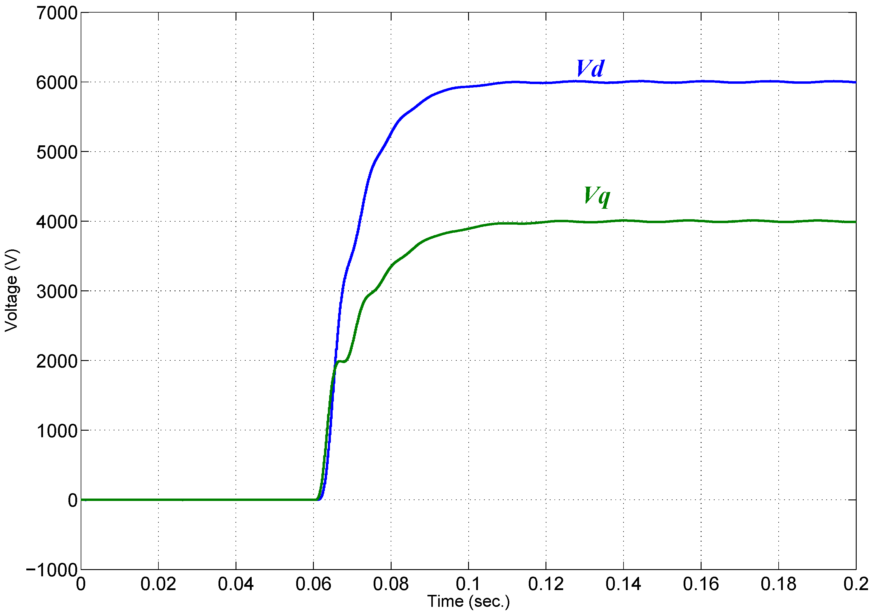
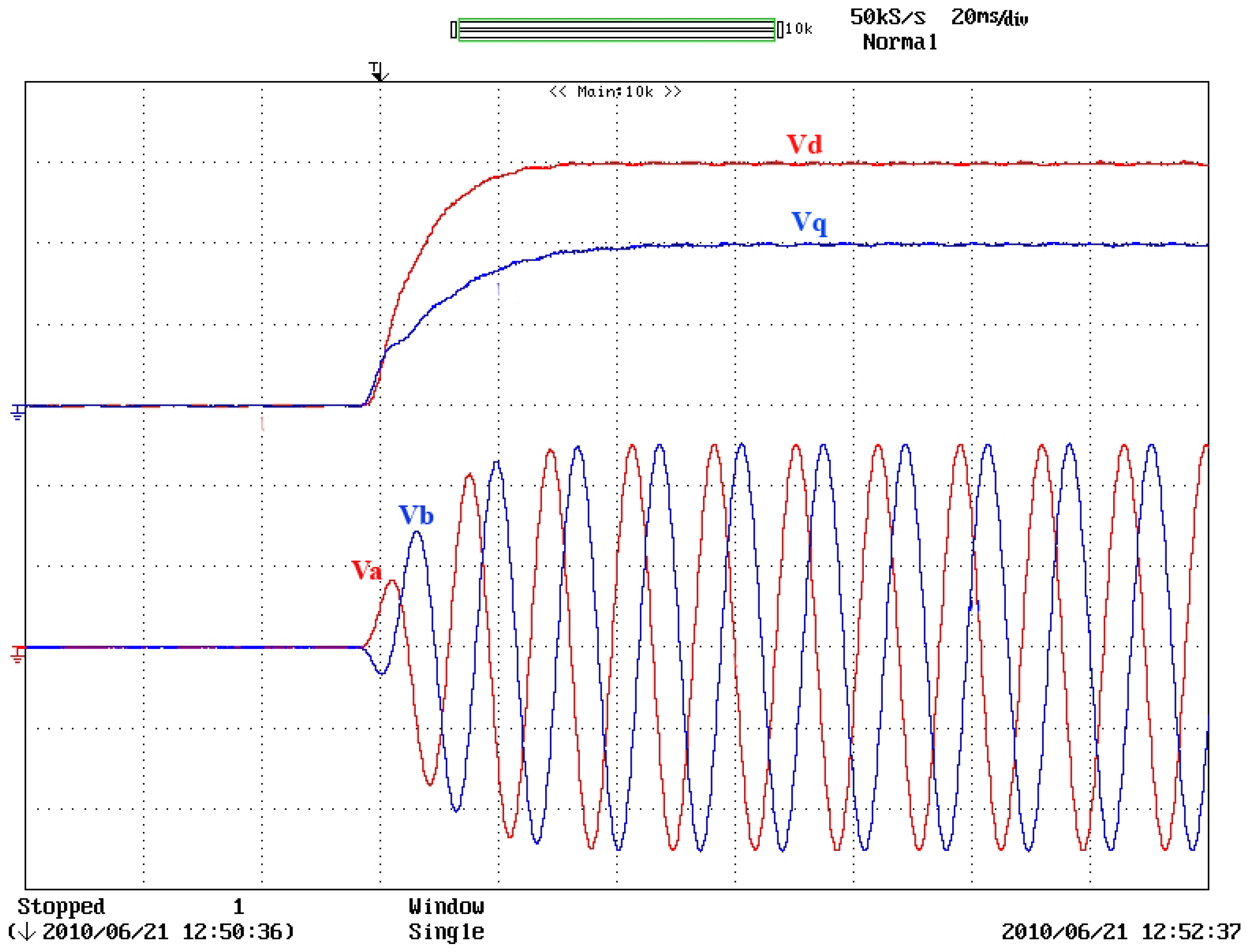
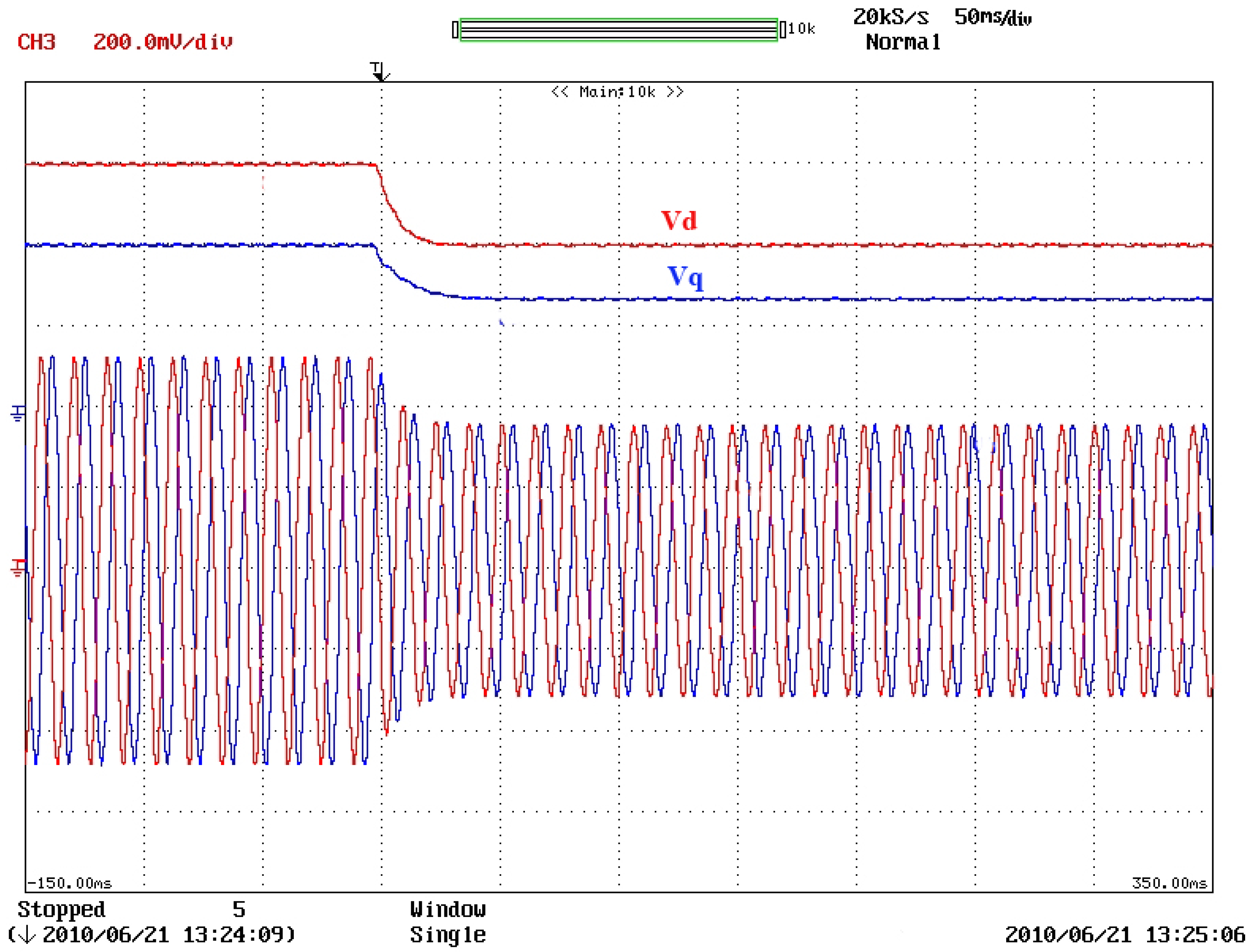
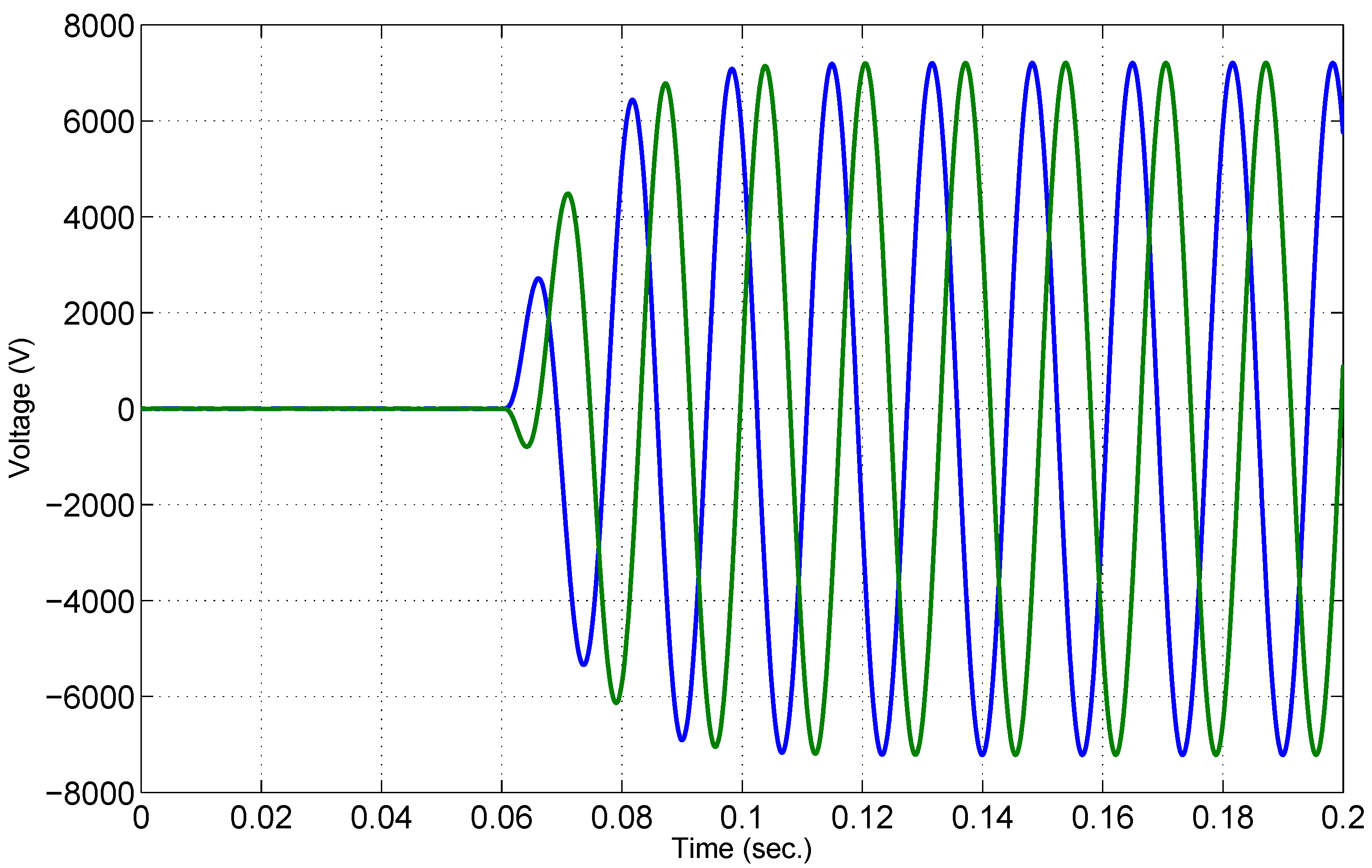
Scenario I: While the system is in the islanded mode with both $V_{dref}$ and $V_{qref}$ set to zero, $V_{dref}$ is stepped up to 6 kV and $V_{qref}$ is stepped up to 4 kV. Figure 8 shows an oscilloscope screen capture of the FPGA-based simulation results corresponding to the d and q components of the load voltage, and the phase a and b voltages of the load. Figure 9 and Figure 10 show the d and q components of the load voltage, and the phase a and b voltages of the load obtained from the Matlab/simpowersystems.

Figure 8. Oscilloscope screen capture of the d and q components of the load voltage, and the phase a and b voltages of the load.

Figure 8. Oscilloscope screen capture of the d and q components of the load voltage, and the phase a and b voltages of the load.

Figure 9. The d and q components of the load voltage generated by the Matlab/simpowersystems.

Figure 9. The d and q components of the load voltage generated by the Matlab/simpowersystems.

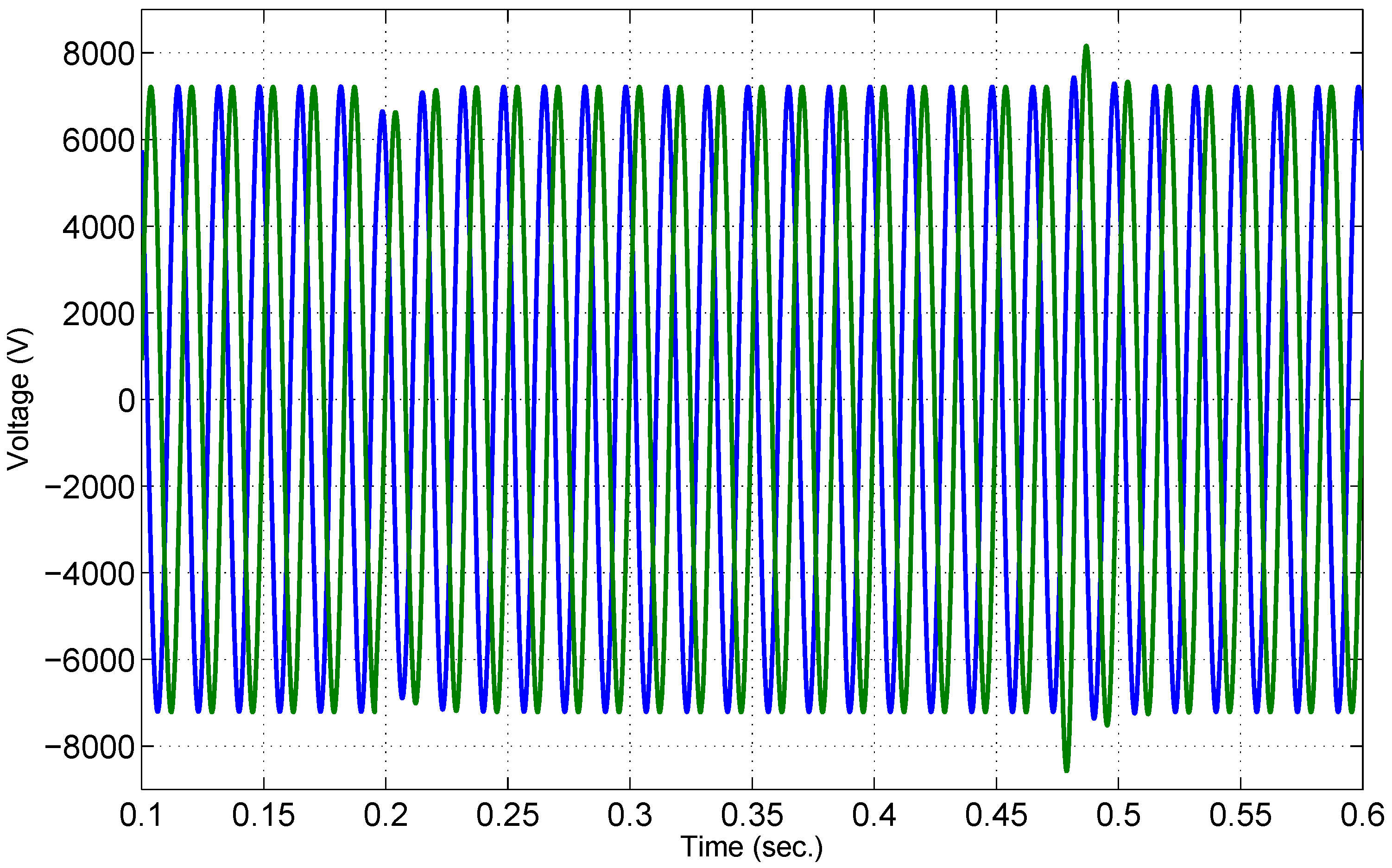
Figure 10. The phase a and b voltages of the load generated by the Matlab/simpowersystems.

Figure 10. The phase a and b voltages of the load generated by the Matlab/simpowersystems.

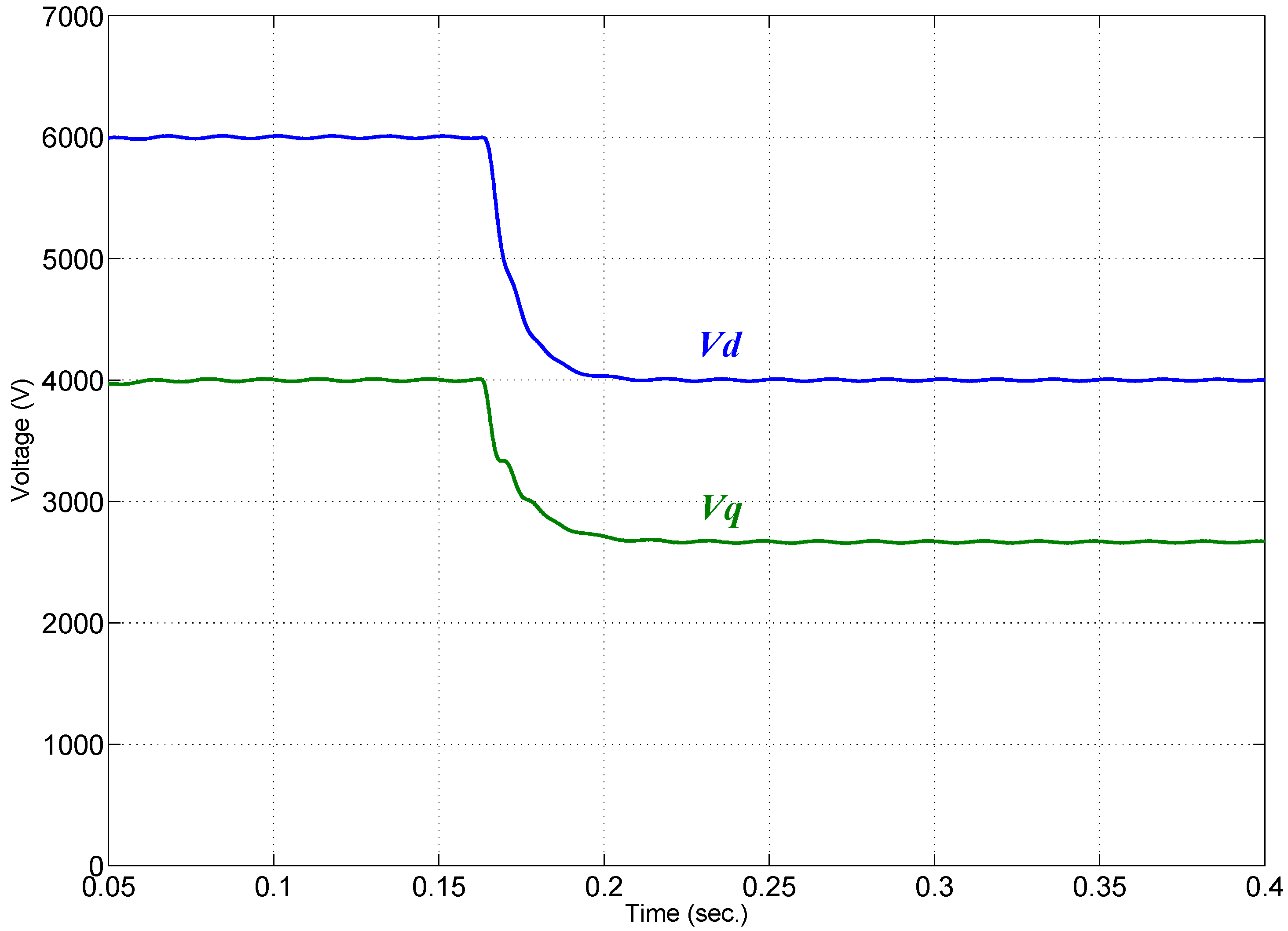
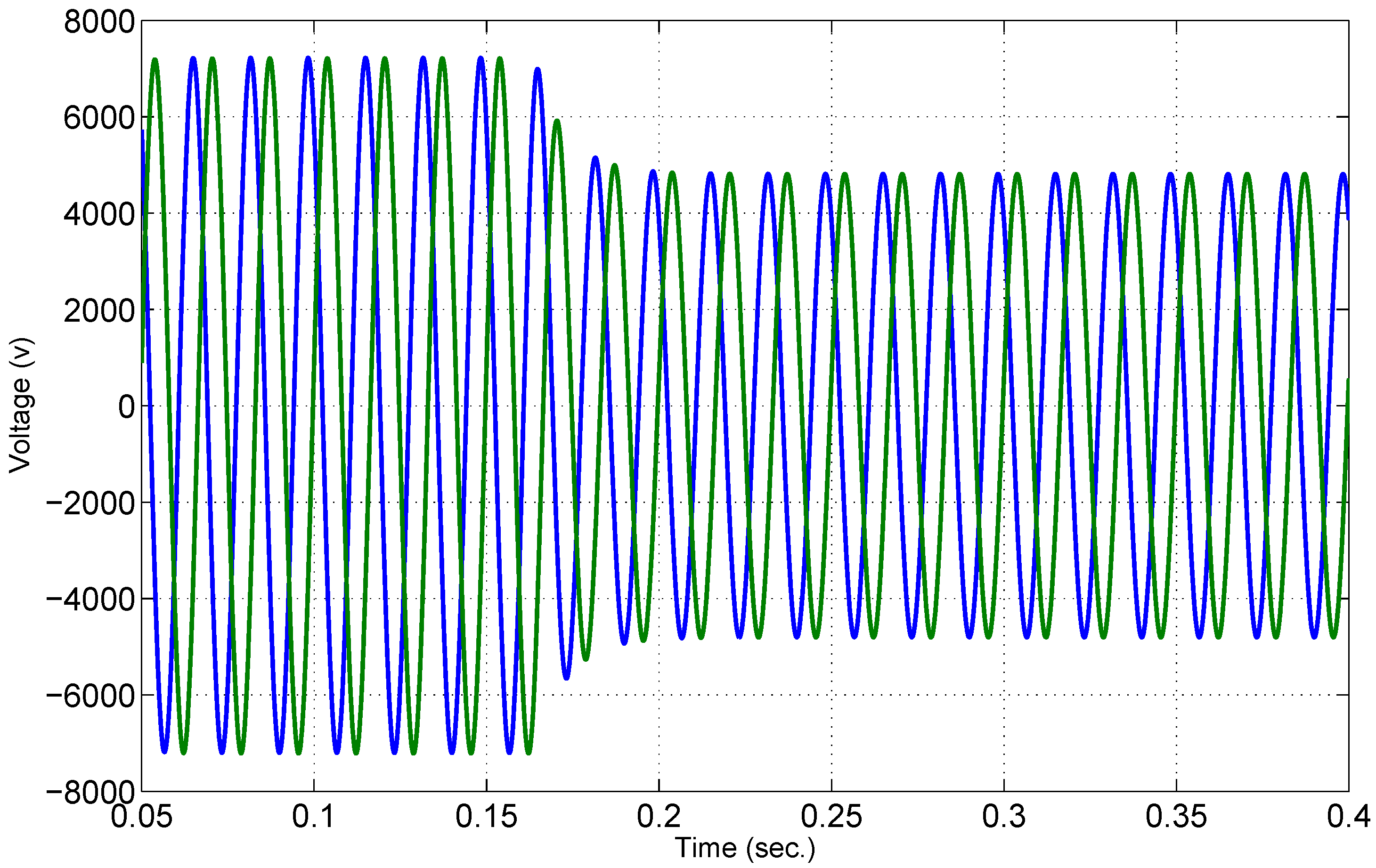
Scenario II: While the system is operating in the islanded mode, in steady state, with $V_{dref}=6$ kV and $V_{qref}=4$ kV, $V_{dref}$ is stepped down to 4 kV and $V_{qref}$ is stepped down to 2.667 kV. Figure 11 shows an oscilloscope screen capture of the FPGA-based simulation results corresponding to the d and q components of the load voltage, and the phase a and b voltages of the load. Figure 12 and Figure 13 show the d and q components of the load voltage, and the phase a and b voltages of the load obtained from the Matlab/simpowersystems.

Figure 11. Oscilloscope screen capture of the d and q components of the load voltage, and the phase a and b voltages of the load.

Figure 11. Oscilloscope screen capture of the d and q components of the load voltage, and the phase a and b voltages of the load.

Figure 12. The d and q components of the load voltage generated by the Matlab/ simpowersystems.

Figure 12. The d and q components of the load voltage generated by the Matlab/ simpowersystems.

Figure 13. The phase a and b voltages of the load generated by the Matlab/simpowersystems.

Figure 13. The phase a and b voltages of the load generated by the Matlab/simpowersystems.

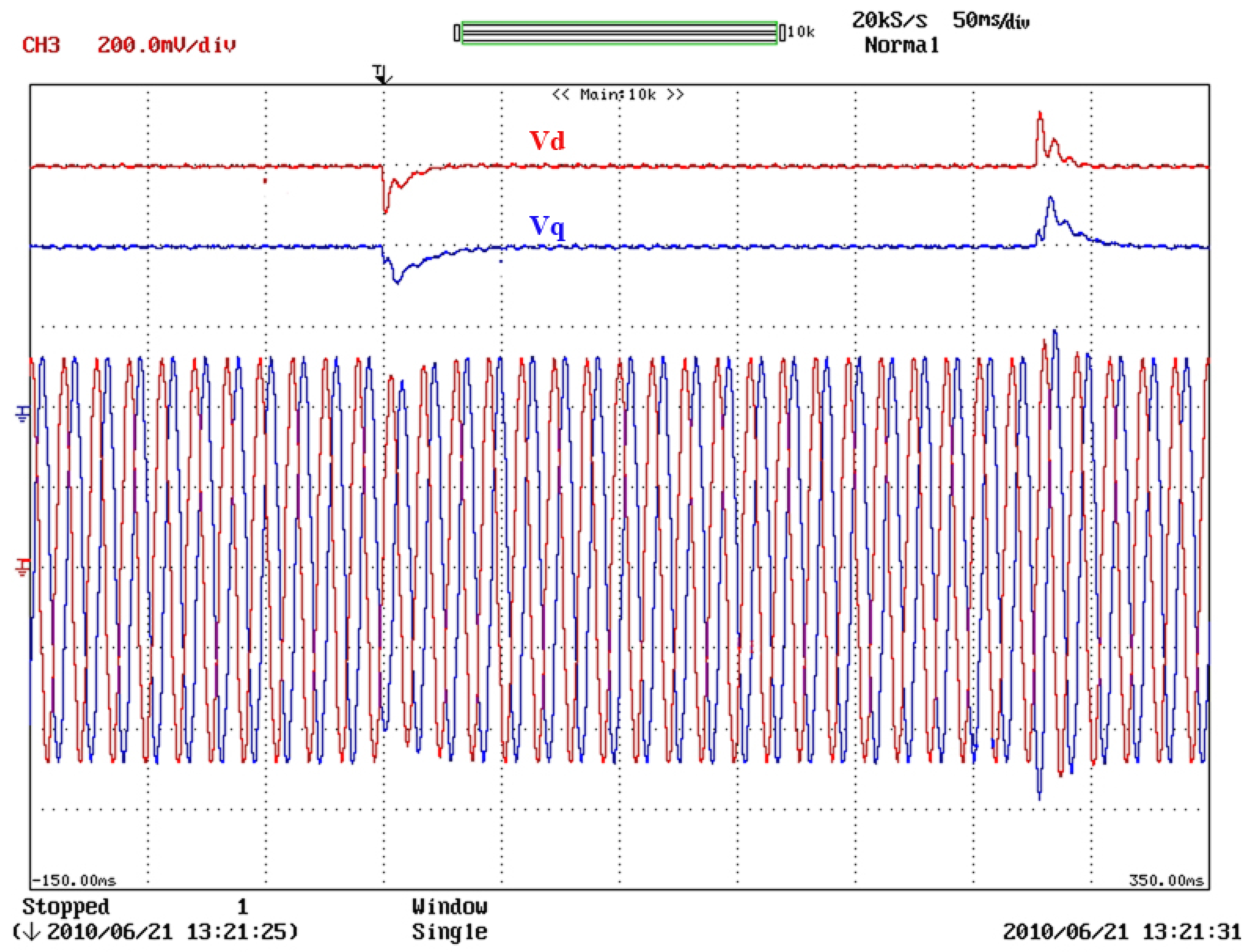
Scenario III: This scenario demonstrates the controller responses to load switchings, both ON and OFF. While the system is operating in the islanded mode, in steady state, with $V_{dref}=6$ kV and $V_{qref}=4$ kV, a resistive load of 76 Ω is switched ON. After the system settles to steady state the resistive load is switched back OFF. Figure 14 shows an oscilloscope screen capture of the FPGA-based simulation results corresponding to the d and q components of the load voltage, and the phase a and b voltages of the load. 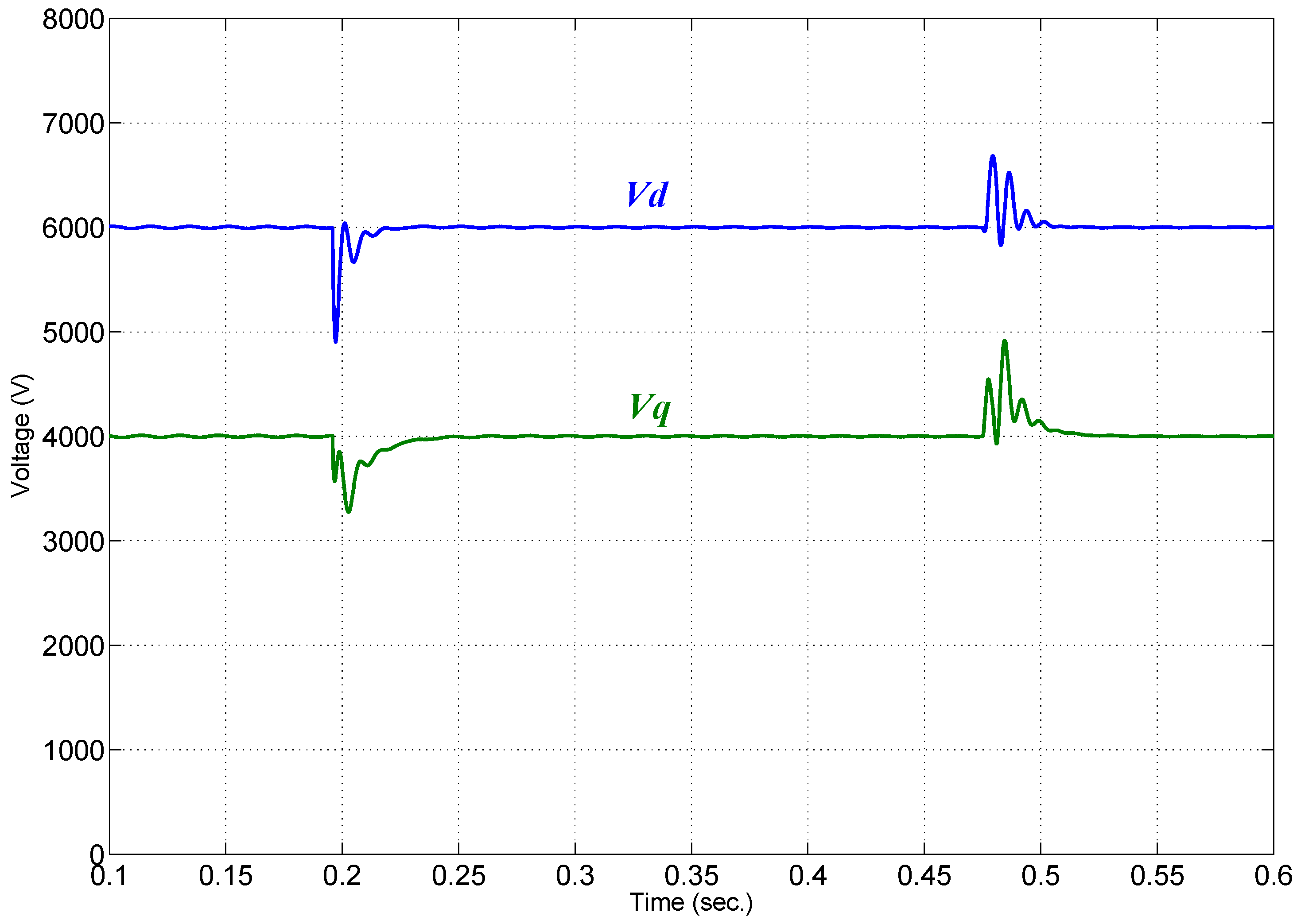Figure 15 and Figure 16 show the d and q components of the load voltage, and the phase a and b voltages of the load obtained from the Matlab/simpowersystems.

Figure 14. Oscilloscope screen capture of the d and q components of the load voltage, and the phase a and b voltages of the load.

Figure 14. Oscilloscope screen capture of the d and q components of the load voltage, and the phase a and b voltages of the load.

Figure 15. The d and q components of the load voltage generated by the Matlab/simpowersystems.

Figure 15. The d and q components of the load voltage generated by the Matlab/simpowersystems.

Figure 16. The phase a and b voltages of the load generated by the Matlab/simpowersystems.

Figure 16. The phase a and b voltages of the load generated by the Matlab/simpowersystems.

Discussions

The close agreement between the corresponding results of Figure 8, Figure 9, Figure 10, Figure 11, Figure 12, Figure 13, Figure 14, Figure 15 and Figure 16 verifies the validity of the FPGA-based real-time simulator to operate in the HIL configuration for testing external controllers. The stability and the accuracy of the simulations for long running durations are also verified as the FPGA-based simulator along with the controller are left continuously running in HIL configuration for hours.

The slight discrepancies between the simulation results obtained from the FPGA-based real-time simulator and those from the Matlab/simpowersystems are due to:

• the delays in the controller outputs imposed by the computation time required by the controller platform to perform the arithmetic calculation of the control algorithm and of the PWM scheme. This delay time is not accounted for in the Matlab/simpowersystems simulation,
• the discretization errors since the Matlab/simpowersystems adopts floating point representation whereas the FPGA-based real-time simulator is based on the fixed point number representation, and
• the errors introduced due to the D/A and A/D converters.

7. Conclusions

This paper presents a high-performance real-time simulator for controller hardware-in-the-loop CHIL testing. The core of the simulator is the novel massively parallel computational engine. The hardware architecture of the computational engine exploits all possible levels of parallelism without imposing severe communication and synchronization overhead times that can limit the performance. The developed simulator enables the real-time simulation of power electronics systems with a nanosecond range simulation timestep, thus eliminating the need to incorporate corrective measures to account for the error arising from the intersimulation timestep switching phenomenon associated with CHIL. The proposed simulator is tested and its CHIL capability verified based on the closed-loop testing of a robust multivariable servomechanism controller for autonomous operation of a distributed generation unit.