1. Introduction
A great part of worldwide energy comes from fossil fuels such as oil derivatives, natural gas and coal. Because of the price increases of fossil fuel resources, their uncertain availability, and environmental concerns, the prediction is that oil exploitation will decrease in the near future. Because of that, total reliance on fossil fuels is not sustainable, and in order to make climate changes and pollution as small as possible, replacement of fossil fuels with biomass is necessary [
1,
2].
Serbia is a country poor in natural reserves of fossil fuels, hence its increased emphasis on direct use of renewable energy sources such as biomass, biogas, wind energy, solar energy, hydropower and geothermal energy [
3]. Biomass has the greatest potential among renewable energy sources. Here, biomass refers to wood biomass and biomass which are the primary agricultural production and food industry residues.
In the face of a significant increase in population worldwide, it is necessary to produce more food to meet present and future demands. Therefore, use of agricultural products, including biomass, for energy purposes can be questionable. With that in mind, this research has been focused on the use of a secondary agricultural product (wheat straw) for energy purposes. Nevertheless, the implications of straw removal on the arable land is another point of discussion. The annual production of primary agricultural residues in Serbia is about 12.4 × 10
6 t. Research [
4] has indicated that, without significant consequences in terms of compromising soil quality (crop plowing increases the humus content in soil and this results in an increase in soil quality), about a quarter of the produced biomass can be taken from the field and used for energy purposes. This means that, in Serbia, about 3.1 × 10
6 t of biomass from agricultural production, which has a potential energy equivalence of 1 × 10
6 t of fuel oil, can be used. The greatest biomass potential comes from corn and wheat and soybean straw. For this reason, research on the appropriate use of biomass for energy purposes have been performed in Serbia. This will significantly reduce the country’s foreign trade deficit and increase profitability and quality of production.
For a comprehensive understanding of the techno-economic determinants of using wheat and soybean straw as a fuel, for selecting and designing the most appropriate technology, plant and equipment for its use of energy, it is necessary to have access to data concerning the thermo-physical and chemical properties of straw that are relevant to the specific conditions of exploitation [
2].
Combustion characteristics of various biomass samples, such as sunflower shell, colza seed, pine cone, cotton refuse and olive refuse are given in [
5]. Applying the derivative thermogravimetry technique, biomass materials showed different combustion characteristics. It should be mentioned that the combustion of the wheat straw can be divided into two stages. One is volatiles emission and combustion, the second is the residual volatiles and fixed carbon combustion [
6].
Straw-fired boiler technology has been proven as an attractive method of disposing of agricultural residues for many years due to its primary advantages of CO
2-neutrality [
7], volume reduction [
8] and energy recovery [
9]. The combustion in an oxygen enriched air atmosphere has the following features: it reduces the available energy loss during the process of translating chemical energy into thermal energy; it decreases the concentration of organic pollutants in the exhaust gas; and it reduces the thermal energy of the exhaust gas to a minimum [
10,
11].
Research on biomass combustion on flat grids is widespread. Zhou
et al. [
12] examined the effect of air preheating and moisture level in the fuel on the combustion characteristics of corn straw. Mass loss rate as a function of time has similar properties as mass loss rate presented in this study. In [
13] the authors presented the development of small-scale batch-fired straw boilers in Denmark in the period from 1995 to 2002. The nominal boiler thermal power was 50–500 kW. One of the emphases was on improvements in boiler efficiency, which were primarily achieved by more installation inside the firebox, by improved techniques for the supply of secondary air and by lowering the flue gas temperature at the boiler outlet pipe. All measured values were recorded every ten seconds by a data logger. In this study, all measured values were recorded every 5 seconds. All stated values obtained during the combustion were averaged values measured throughout the entire combustion period like in this study. The minimum average boiler thermal power was 63 kW, with an average efficiency of 75%, while the maximum average boiler thermal power was 461 kW with an average efficiency of 88%. In [
14], the authors presented an experimental investigation into the combustion behavior of straw in a fixed bed combustor. Among others, they analyzed the effects of a crucial combustion parameter, primary air flow rate, on straw combustion. They reported that bale mass loss was the slowest at an air flow of 234 kg m
−2 h
−1 and that there was an exponential dependence of mass loss on bale residence time. The mass loss was the fastest at an air flow of 702 kg m
−2 h
−1, where a linear decrease occurred after the bed was ignited by the start-up burner.
Some research has included formulation of mathematical models. Zhou
et al. [
15], created a one-dimensional unsteady heterogeneous mathematical model based on straw combustion in a fixed bed. A 3D mathematical model of straw combustion can be found in Zhaosheng
et al. [
16]. Combustion product composition (especially CO and CO
2) was examined in Bubenheim
et al. [
17].
The goal of this study was to examine the influence of the quantity of inlet air and recirculation of combustion products on the boiler thermal power and boiler energy efficiency. Recirculation of combustion products of p% means that out of 100% quantity of inlet air fed to the boiler firebox, p% is warm air created from the combustion products and the rest is fresh air. Another aim is to formulate the equations which will represent the boiler thermal power and boiler energy efficiency dependence on wheat straw bale residence time.
2. Material and Methods
2.1. Boiler Plant and Measurement Points
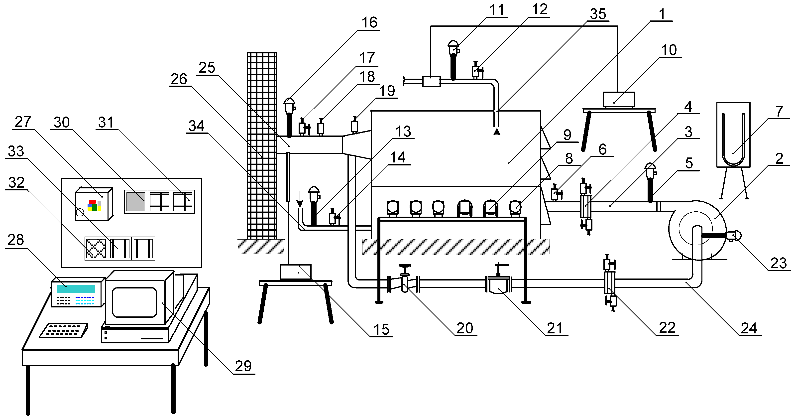
This study describes a boiler plant for the combustion of wheat straw bales (
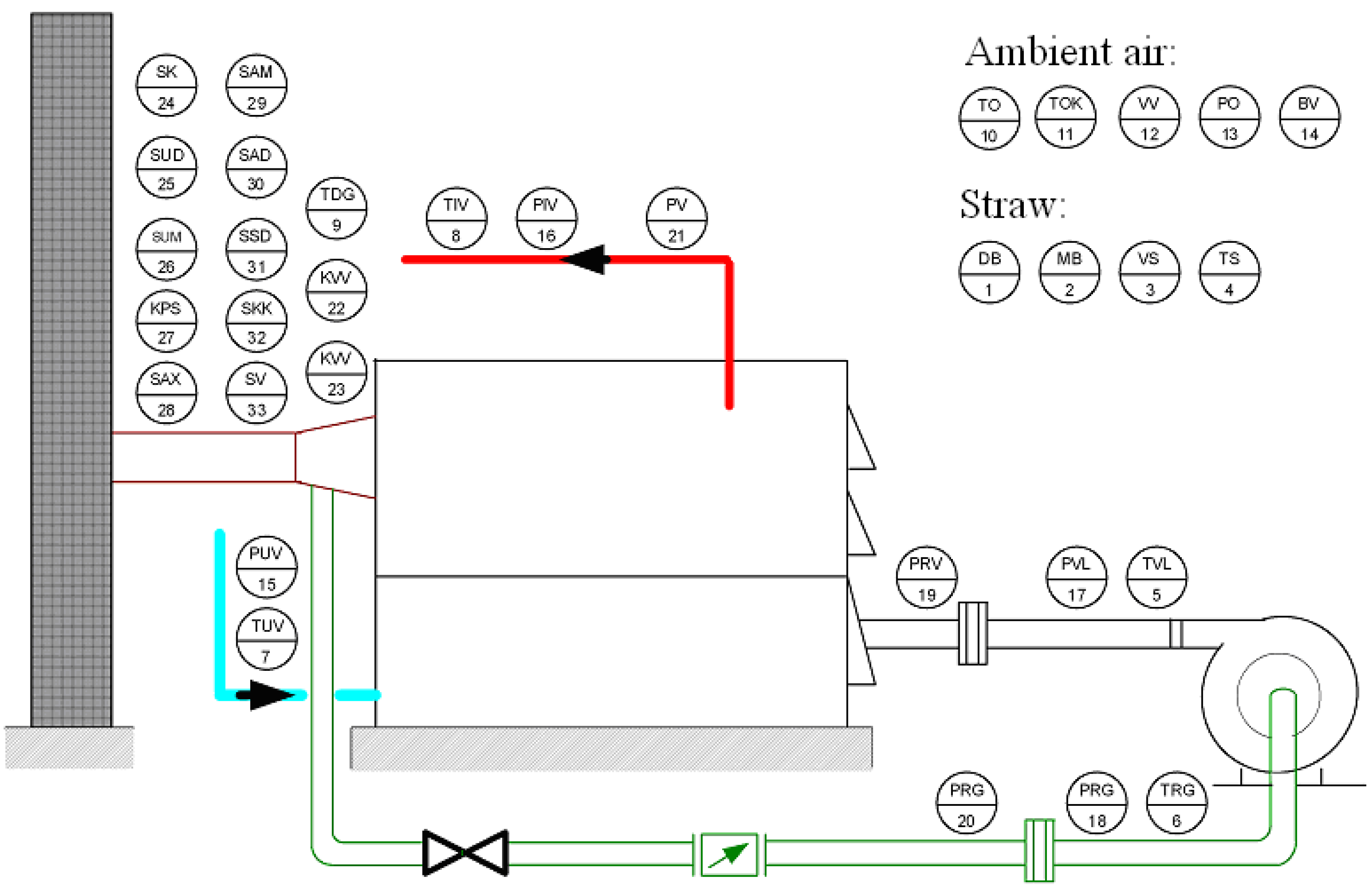
Figure 1). The plant is located at the “Mitrosrem” agricultural company’s “Kuzmin” working-unit in the town of Sremska Mitrovica (Longitude: 19°36'39'' E, Latitude: 44°58'6'' N). The plant’s central point is a hot-water manually fed boiler with a nominal power of 120 kW.
The boiler plant consists of several separate, but interconnected functional units which contain the necessary equipment for measurement and regulation. The functional units which make up the boiler plant are the following: supply pipe, measurement and regulation of the amount of fresh air which is fed into the firebox, combustion of bio-fuels and transfer of the produced thermal power, combustion products disposal and measurement and regulation equipment.
Figure 1.
Boiler plant of the “Ekoprodukt” manufacturer from Novi Sad with its measurement and regulation equipment (1-hot-water boiler, 2-combustion air fan, 3-tube for air supply into the combustion chamber, 4-airflow differential pressure meter with orifice plates (conic edge), 5-Pt100 temperature sensor for measuring air temperature, 6-sensor for measuring pressure of combustion air, 7-“U” tube, 8-differential pressure transmitters, 9-pressure transmitter, 10-ultrasonic water flowmeter, 11-Pt100 temperature sensor for measuring the temperature of output water, 12-sensor for measuring pressure of output water, 13-Pt100 temperature sensor for measuring the temperature of inlet water, 14-sensor for measuring pressure of incoming water, 15-flue gas analyzer, 16-thermocouples for measuring flue gas temperature, type K (Ni-CrNi), 17-sensor for measuring pressure of flue gas, 18-oxygen lambda sensor without heater, 19-oxygen lambda sensor with heater, 20-shut-off valve, 21-gate valve, 22-airflow differential pressure meter with orifice plates (conic edge), 23-Pt100 temperature sensor for measuring the temperature of flue gas recirculation, 24tube for intake of recirculation flue gas, 25-flue gas canal, 26-chimney, 27-frequency regulator for combustion air fan, 28-controller, 29-personal desktop computer, 30-expansion adapter EX-A1, 31-expansion module IO-PT4, 32-expansion module IO-ATC8-, 33-expansion module IO-AI4-AO2, 34-tube of inlet water supply, 35-tube of output water).
![Energies 05 01470 g001]()
The tests were conducted during March and April 2011. The measurement results were automatically recorded in a controller every five seconds, thus enabling the continuous monitoring of the combustion process. Under the same circumstances, combustion of straw bales was repeated three times per each regime. Before we started with the experiments, we had carried out screening experiments to determine the time when the bale completely burnt out. We have visually determined that when the bale completely burnt out, the excess air ratio was about 7. Therefore, combustion experiments were interrupted when the excess air ratio surpassed 7. Experimental measurements were conducted using the instruments given in
Table 1.
Table 1.
Summary of measurement points and instruments.
Table 1.
Summary of measurement points and instruments.
| No. of meas. | Meas. design. | Measurement value | | Type of instrument | Meas. range | Meas. accuracy and resolution |
|---|
| 1. | DB | Straw bale dimension | | Strain gauge | - | - |
| 2. | MB | Straw bale mass | | “Labela-preciz” scale | 0–50 kg | ±0.020 kg |
| 3. | VS | Straw humidity contents | | Laboratory dryer and “Sartorius” scale | 0–120 g | ±0.001 kg |
| 4. | TS | Incineration time for straw bale | | Manual stopwatch | - | - |
| 5. | TVL | Firebox inlet air temperature | | Temperature probe type Pt-100 | 0–400 °C | 0.1 °C |
| 6. | TRG | Temperature of the recirculated combustion products | | Temperature probe type Pt-100 | 0–400 °C | 0.1 °C |
| 7. | TUV | Boiler inlet water temperature | | Temperature probe type Pt-100 | 0–400 °C | 0.1 °C |
| 8. | TIV | Boiler outlet water temperature | | Temperature probe type Pt-100 | 0–400 °C | 0.1 °C |
| 9. | TDG | Flue gas temperature | | Temperature probe type K (Ni-CrNi) | 0–1200 °C | 0.1 °C |
| 10. | TO | Environment temperature | | Republic of Serbia hydrometeorological service | - | 0.1 °C |
| 11. | TOK | Environment temperature | | Temperature probe type Pt-100 | 0–400 °C | 0.1 °C |
| 12. | VV | Environment humidity | | Republic of Serbia hydrometeorological service | - | - |
| 13. | PO | Environment air-pressure | | Republic of Serbia hydrometeorological service | - | 0.1 mbar |
| 14. | BV | Wind speed | | Republic of Serbia hydrometeorological service | - | - |
| 15. | PUV | Boiler inlet water pressure | | Pressure transmitter type SITRANS DSIII | 0–10 bar | 0.1 mbar |
| 16. | PIV | Boiler outlet water temperature | | Pressure transmitter type SITRANS DSIII | 0–10 bar | 0.1 mbar |
| 17. | PVL | Firebox inlet air pressure | | SITRANS DSIII differential pressure transmitter | 0–1600 mbar | 0.1 mbar |
| 18. | PRG | Combustion products pressure | | SITRANS DSIII differential pressure transmitter | 0–1600 mbar | 0.1 mbar |
| 19. | PRV | Firebox inlet air throughput | | Standard muffler and SITRANS DSIII differential pressure transmitter | 0–1600 mbar | 0.1 mbar |
| 20. | PRG | Recirculated combustion products throughput | | Standard muffler and SITRANS DSIII differential pressure transmitter | 0–1600 mbar | 0.1 mbar |
| 21. | PV | Boiler water throughput | | Yokogawa type US300PM ultrasound throughput probe | | |
| 22. | KVV | Air excess rate 1 | | Universal lambda probe Bosch LS 01 | 0–1.1 V | 0.01 V |
| 23. | KVV | Air excess rate 2 | | Universal lambda probe with heater Bosch LS 01 | 0–1.1 V | 0.01 V |
| 24. | SK | O2 content in combustion products | | TESTO 350 XL combustion analyser | 0–21% | - |
| 25. | SUD | CO2 content in combustion products | | TESTO 350 XL combustion analyser | 0–20.5% | 0.2% |
| 26. | SUM | CO content in combustion products | | TESTO 350 XL combustion analyser | 0–10,000 ppm | 1 ppm |
| 27. | KPS | Air excess rate in combustion products | | TESTO 350 XL combustion analyser | - | - |
| 28. | SAX | NOx content in combustion products | | TESTO 350 XL combustion analyser | - | - |
| 29. | SAM | NO content in combustion products | | TESTO 350 XL combustion analyser | 0–3000 ppm | 1 ppm |
| 30. | SAD | NO2 content in combustion products | | TESTO 350 XL combustion analyser | 0–500 ppm | 0.1 ppm |
| 31. | SSD | SO2 content in combustion products | | TESTO 350 XL combustion analyser | 0–5000 ppm | 1 ppm |
| 32. | SKK | Efficiency in combustion products | | TESTO 350 XL combustion analyser | - | - |
| 33. | SV | H2 content in combustion products | | TESTO 350 XL combustion analyser | - | - |
Locations where measurements were taken are shown in
Figure 2. Measured values are marked according to their labels listed in
Table 1.
Figure 2.
Layout of measurement points.
Figure 2.
Layout of measurement points.
2.2. Wheat Straw Characteristics
For the purpose of this study, prismatic wheat straw bales were used. The straw collection was conducted right after the harvest. The straw was baled with a press, and stored in piles in the agricultural courtyards of the working-unit. In laboratory terms, the average heating value of wheat straw was 13.48 MJ kg
−1 (moisture content 8.2%). After drying, it was 14.9 MJ kg
−1. In laboratory terms the average value of the quantity of wheat straw ashes was 6.2% [
18]. Composition of wheat straw biomass from Serbia is given in
Table 2 [
19].
Table 2.
Chemical composition of wheat straw from Serbia.
Table 2.
Chemical composition of wheat straw from Serbia.
| | | Content | | | Content | |
|---|
| Ash | | 7.9% | | Aluminum | 240 mg kg−1 | |
| Carbon | | 42.9% | | Calcium | 1720 mg kg−1 | |
| Chlorine | | 0.17% | | Iron | 240 mg kg−1 | |
| Hydrogen | | 5.7% | | Magnesium | 620 mg kg−1 | |
| Nitrogen | | 0.62% | | Manganese | 40 mg kg−1 | |
| Oxygen | | 38.25% | | Phosphorus | 700 mg kg−1 | |
| Sulfur | | 0.16% | | Potassium | 10,440 mg kg−1 | |
| Water | | 4.3% | | Silicon | 34,090 mg kg−1 | |
Bales of approximately the same size and weight were selected. Upon selection they were stored in the warehouse of the “Kuzmin” working-unit. Altogether, 350 wheat straw bales were selected. They were stored in a warehouse near the boiler plant so they were not exposed to additional climate effects, which helped in preserving their quality and prevented deterioration of the content, shape and the level of compactness. The average cross-cut of the wheat bales was 0.35 m × 0.5 m, whereas the average length was 0.75 m. The compactness was rather equal. During each experiment, one wheat straw bale was burnt.
2.3. Operating Regimes
This study shows different boiler operating regimes (the amount of air fed into a boiler varied). The effects of four different operating regimes (220, 290, 360 and 430 m
3 h
−1) on the combustion process are described. The amount of air fed into the firebox during the combustion process influences on the energy efficiency rate of the boiler that runs on biomass. Measurement methods are in accordance with the SRPS EN 303-5:2007 standards and DIN 4702 in boiler thermal power determination. Boiler thermal power was determined using a direct method [
18],
i.e., by measuring the volume of water supplied and by measuring the water temperature at the boiler entrance and exit points. A detailed overview (measuring codes, bale dimensions, instrument names, measuring ratio) is also given in [
20,
21]. During the experiments, boiler thermal power was determined based on the following formula [
22]:
where
P is the boiler thermal power,
mass flow of water through the boiler (m
3 h
−1),
cp specific heat of water,
tiv boiler outlet water temperature,
tuv boiler inlet water temperature. Energy efficiency rate of a boiler was determined by [
22]:
where
η(
τ) is energy efficiency rate,
P is the boiler thermal power,
m0–bale mass (kg),
m(
τ)–bale mass at time τ (kg),
hd heating value of fuel (kJ kg
−1),
tiv boiler outlet water temperature,
tuv boiler inlet water temperature.
2.4. Statistical Analysis
Mathematical models were obtained from experimental data and application of nonlinear regression analysis. Regression analysis comprises the following: the choice of appropriate regression function f(x1,x2,...)=φ(β1,β2,...,x1,x2,...), where β1,β2,... are regression coefficients, and x1,x2,... are independent variables; evaluation of regression coefficients β1,β2,..., that is, determining their approximate values b1,b2,... in order for the function φ(b1,b2,...,x1,x2,...) to represent as close as possible approximation of regression function f(x1,x2,...). Coefficients b1,b2,... are called empirical regression coefficients; statistical analysis of the obtained approximation (precision in prediction, regression coefficient intervals, etc.).
The compatibility of mathematical models with the measured data is checked with the following tests:
t-test examines the regression coefficients’ significance,
F-test determines the significance of factors effects on dependent variables,
i.e., whether the set model is significant, the level of determination of dependent variables is shown through the coefficient of determination
R2 for the chosen independent variables and it shows the compatibility of the curves to the results [
23].
This study contains the following mathematical models and formulas: correlation between boiler thermal power and bale residence time; correlation between boiler energy efficiency and bale residence time; bale mass loss during the combustion process. These models are presented for all regimes and all types of combustion products recirculation.
3. Results and Discussion
This research shows the mathematical models resulting from the average values of combustion parameter experiments (boiler thermal power and boiler energy efficiency) repeated three times at every operating regime with 0, 16.5 and 33% recirculation. The average time when bale totally burnt, as well as the average values of boiler thermal power and energy efficiency rate, during the whole combustion process are presented in
Table 3. Intervals of standard error of average boiler thermal power and energy efficiency in percentages are also presented.
Table 3.
Combustion process results with intervals of standard error in percentages.
Table 3.
Combustion process results with intervals of standard error in percentages.
| | Rec. | Boiler operating regime (m3 h−1) |
|---|
| 220 | 290 | 360 | 430 |
|---|
| Average time when bale totally burnt (s) with standard error (%) | 0% | 1055 (6.58) | 947 (0.88) | 650 (2.80) | 587 (2.50) |
| 16.5% | 1427 (5.06) | 1312 (2.73) | 772 (4.67) | 698 (4.00) |
| 33% | 1185 (6.04) | 955 (3.42) | 710 (2.09) | 632 (2.80) |
| Average boiler thermal power (kW) with intervals of standard error (%) | 0% | 63.47 (0.27, 12.15) | 71.75 (0.73, 11.44) | 88.21 (0.44, 13.36) | 90.90 (1.05, 12.76) |
| 16.5% | 57.86 (0.40, 10.22) | 68.88 (1.38, 11.69) | 81.44 (0.17, 10.08) | 88.12 (0.42, 9.03) |
| 33% | 55.65 (0.35, 12.45) | 67.79 (0.27, 6.31) | 72.82 (0.91, 10.12) | 84.98 (0.25, 4.90) |
| Average boiler energy efficiency rate (%) with intervals of st. error (%) | 0% | 57.94 (0.03, 12.89) | 60.00 (1.08, 11.08) | 39.45 (1.05, 12.76) | 36.57 (0.08, 12.47) |
| 16.5% | 66.08 (0.14, 11.33) | 52.83 (0.20, 13.73) | 45.50 (1.01, 9.39) | 42.60 (0.29, 8.45) |
| 33% | 49.85 (0.59, 11.46) | 41.64 (0.24, 5.63) | 44.01 (1.84, 10.26) | 41.77 (0.57, 7.15) |
General conclusions are: (1) increase of inlet air fed to the boiler firebox produces a combustion time decrease and an increase of boiler thermal power; (2) combustion product recirculation increases bale residence time and decreases average boiler thermal power; (3) in the 220 and 290 m3 h−1 regimes average boiler energy efficiency is greater than 50% if recirculation is 0 or 16.5%; (4) in the 360 and 430 m3 h−1 regimes average boiler energy efficiency is very small; (5) maximum average boiler energy efficiency (66.08%) is reached in the 220 m3 h−1 regime if recirculation is 16.5% and after that (60%) in the 290 m3 h−1 regime if there is no recirculation; (6) in the 360 and 430 m3 h−1 regimes with 16.5 and 33% recirculation average boiler energy efficiency is increased compared to the efficiency when there is no recirculation. This is due to a relatively small change in boiler thermal power and higher bale residence time; (7) comparing recirculation of 16.5 and 33%, it can be seen that first one provides better boiler characteristics regarding all considered parameters.
3.1. Boiler Thermal Power–Experimental Data and Mathematical Model
Our first task was to express boiler thermal power as a function of air flow and bale residence time. Therefore, according to
Figure 3(a), it can be concluded that for higher air flow (360 and 430 m
3 h
−1), experimental data should be approximated by an exponential function exp(−(
x −
a)
2) which is symmetric with respect to the line
x =
a and its graphical interpretation fits a normal distribution (
a serves for graph translation along the
x-axis). One can see that: (a) higher air flow
implies higher maximum boiler thermal power
P (so the regression coefficients
b and
should multiply the function exp(−(
x −
a)
2) and we obtain
b·
·exp(−(
x −
a)
2); (b) higher air flow
makes the time
τkr when the bale is totally burnt shorter and the graph becomes narrower. Thus, function
b·
·exp(−(
c(
x −
a)/
τkr)
2) should properly approximate the experimental data for higher regimes. Regression coefficients
a,
b and
c are useful for graph corrections according to experimental data. For lower air flows (220 and 290 m
3 h
−1), experimental data should be approximated by a function of the type
·sin((
x −
b)/
τkr), with the same arguments as stated above. Finally, a mathematical model of the correlation between boiler thermal power and bale residence time for different operating regimes is formed on the basis of the model in [
3] and it is given in (1):
Here,
b1,
b2,...,
b7 are regression coefficients given in
Table 4a, 4b and 4c,
τ is the bale residence time,
P is the boiler thermal power,
is air flow and
τkr is the time when the bales are totally burnt.
Table 4.
Estimation of empirical regression coefficients and analysis of variance of model (1), (a) no recirculation; (b) recirculation 16.5%; (c) recirculation 33%.
Table 4.
Estimation of empirical regression coefficients and analysis of variance of model (1), (a) no recirculation; (b) recirculation 16.5%; (c) recirculation 33%.
| (a) Level of confidence: 95%, Determination coefficient: R2 = 90.40% |
|---|
| | Estimate | Standard error | t-test | Confidence interval | | | Sum of squares | F-test |
|---|
| b1 * | 44.328 | 0.6385 | 69.4 | (43.074, 45.581) | | Regression | 5,007,404 | 14,755 |
| b2 * | 0.0876 | 0.0039 | 22.1 | (0.0798, 0.0953) | Residual | 42,955 |
| b3 * | 4.2476 | 0.1585 | 26.8 | (3.9364, 4.5588) | Total | 5,050,359 |
| b4 * | 330.85 | 4.1294 | 80.1 | (322.75, 338.96) | | | |
| b5 * | 0.1176 | 0.0037 | 32.1 | (0.1104, 0.1248) |
| b6 * | 3.3293 | 0.0458 | 72.6 | (3.2394, 3.4193) |
| b7 * | 77.749 | 5.1614 | 15.1 | (67.619, 87.879) |
| (b) Level of confidence: 95%, Determination coefficient: R2 = 82.08% |
| | Estimate | Standard error | t-test | Confidence interval | | | Sum of squares | F-test |
| b1 * | 21.251 | 0.6520 | 32.6 | (19.971, 22.531) | | Regression | 3,358,095 | 18,704 |
| b2 * | 0.1709 | 0.0039 | 43.4 | (0.1638, 0.1788) | Residual | 15,184 |
| b3 * | 4.1108 | 0.0837 | 49.1 | (3.9459, 4.2747) | Total | 3,373,279 |
| b4 * | 345.90 | 2.0554 | 168.3 | (341.86, 349.93) | | | |
| b5 * | 3.0907 | 0.0678 | 47.2 | (2.9321, 3.1723) |
| b6 * | 0.0387 | 0.0021 | 6.4 | (0.0031, 0.0043) |
| b7 * | −165.18 | 1.0112 | −6.4 | (−216.20, −114.16) |
| (c) Level of confidence: 95%, Determination coefficient: R2 = 85.23% |
| | Estimate | Standard error | t-test | Confidence interval | | | Sum of squares | F-test |
| b1 * | 3.1984 | 1.0089 | 3.2 | (1.2182, 5.1786) | | Regression | 3,493,165 | 9758 |
| b2 * | 0.3696 | 0.0063 | 59.1 | (0.3573, 0.3819) | Residual | 44,081 |
| b3 * | 2.5268 | 0.0481 | 52.6 | (2.4324, 2.6211) | Total | 3,537,245 |
| b4 * | 261.53 | 5.4777 | 47.7 | (250.77, 272.28) | | | |
| b5 * | 0.1438 | 0.0041 | 34.8 | (0.1357, 0.1519) |
| b6 * | 4.3694 | 0.0753 | 57.9 | (4.2215, 4.5173) |
| b7 * | 470.58 | 6.0233 | 78.1 | (458.76, 482.40) |
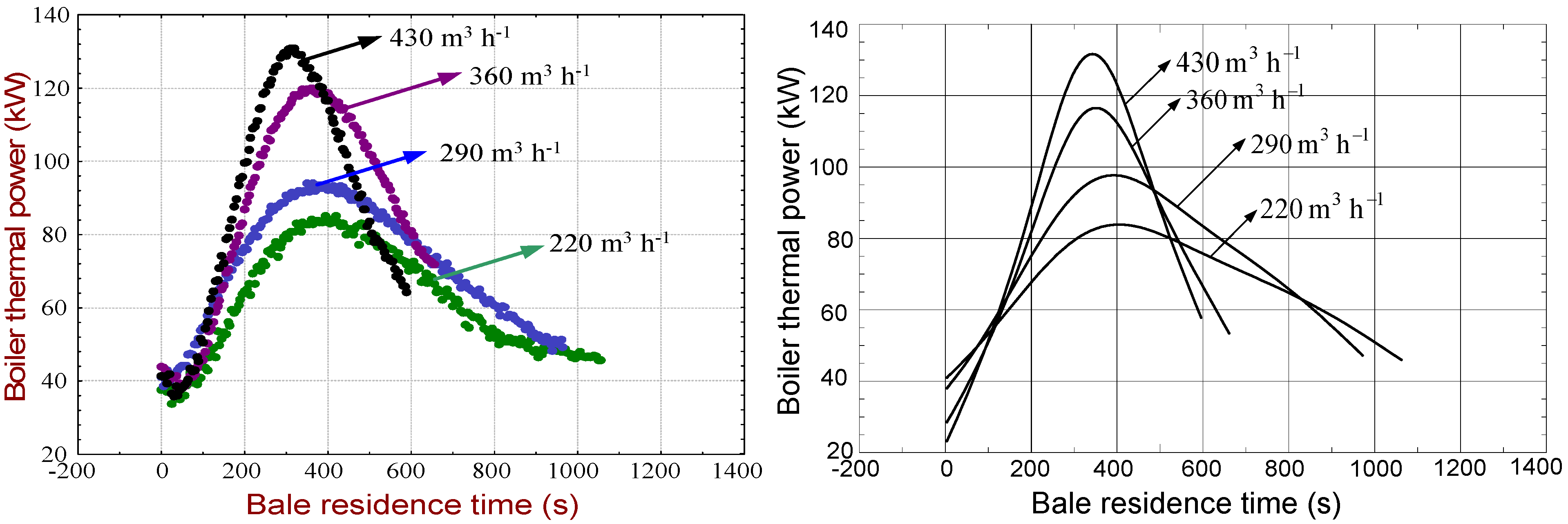
Experimental data of boiler thermal power and its graphical interpretation based on formula (1) are given in
Figure 3(a) and 3(b) (for the case of recirculation 0%). If there is no combustion products recirculation into the firebox, then two operating regimes can be regarded as the optimal ones (220 and 290 m
3 h
−1) regarding to boiler thermal power values and time when bale totally burnt. At the operating regime 220 m
3 h
−1, the maximum boiler thermal power was 84.05 kW with
τkr = 1055 s. At the operating regime 290 m
3 h
−1, the maximum boiler thermal power was 97.97 kW and
τkr = 947 s.
Figure 3.
(a) Correlation between boiler thermal power and bale residence time, experimental data, recirculation 0%; (b) Correlation between boiler thermal power and bale residence time, model (1), recirculation 0%.
Figure 3.
(a) Correlation between boiler thermal power and bale residence time, experimental data, recirculation 0%; (b) Correlation between boiler thermal power and bale residence time, model (1), recirculation 0%.
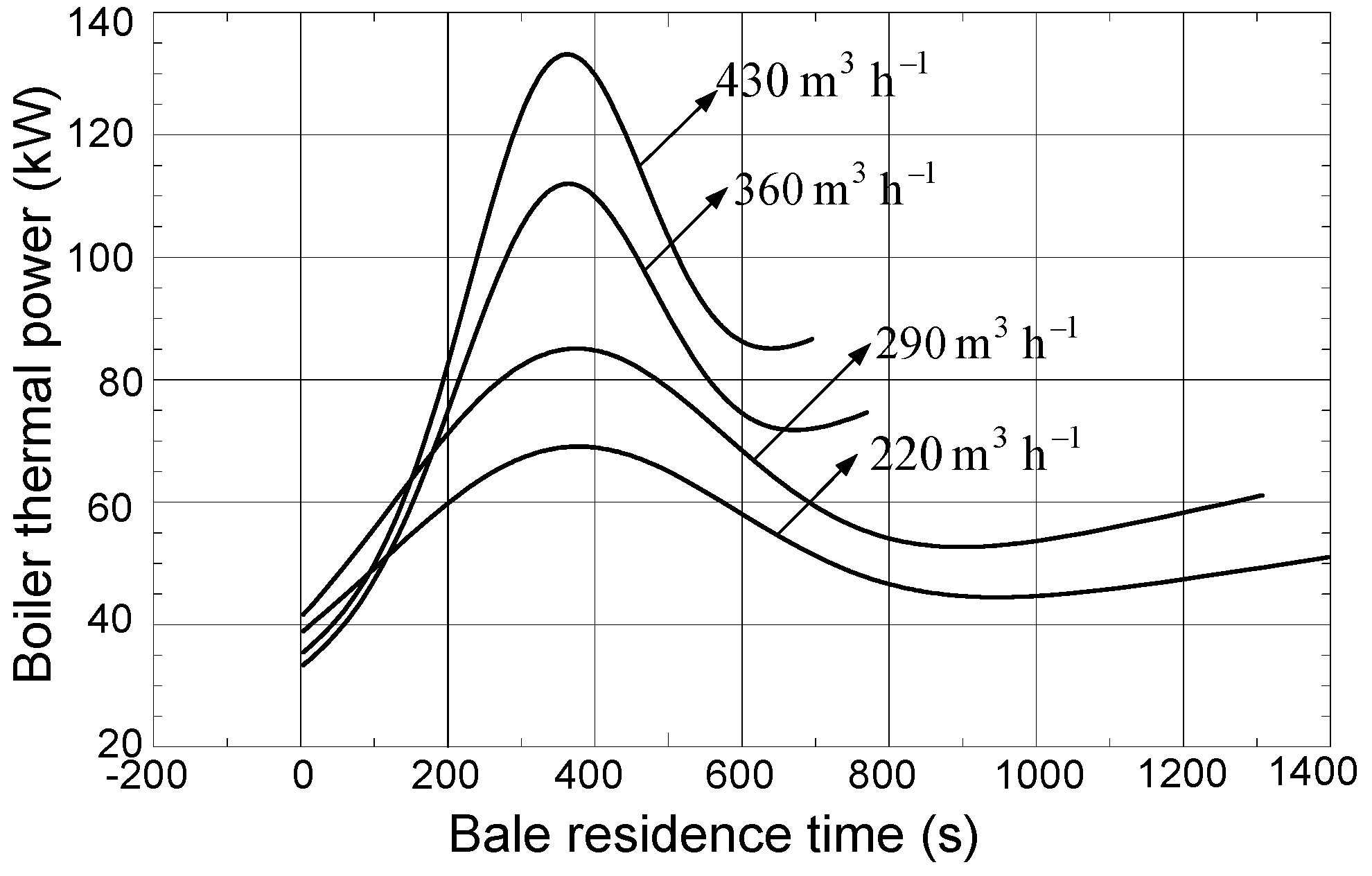
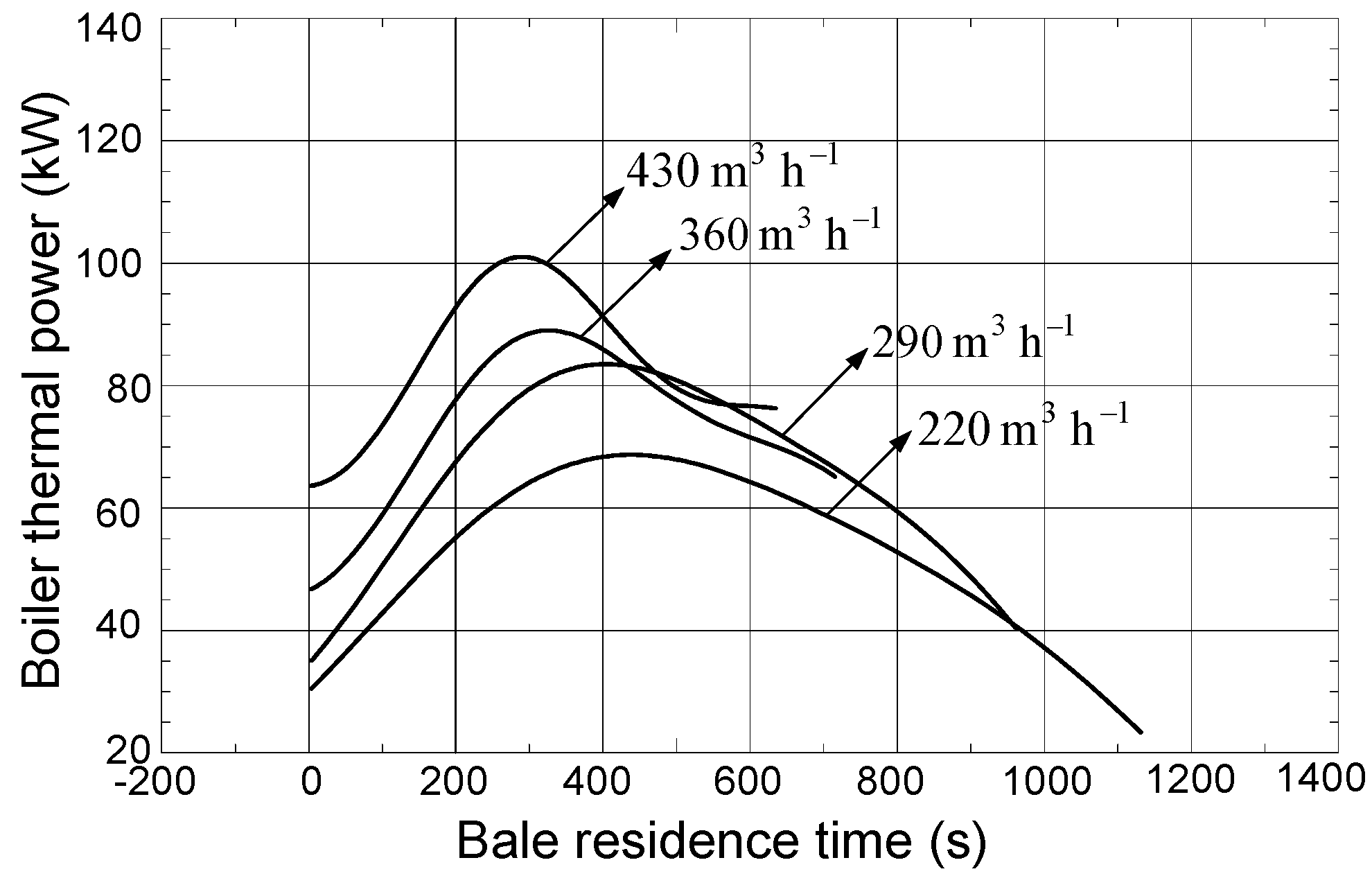
Graphical interpretation for two other recirculation types can be seen in
Figure 4 and
Figure 5. If the combustion products recirculation of 16.5% (or 33%) occurs, then the time when bale was totally burnt was prolonged, but the average thermal boiler power was smaller compared to the case when recirculation is 0% (
Table 3).
Figure 4.
Correlation between boiler thermal power and bale residence time, model (1), recirculation 16.5%.
Figure 4.
Correlation between boiler thermal power and bale residence time, model (1), recirculation 16.5%.
Figure 5.
Correlation between boiler thermal power and bale residence time, model (1), recirculation 33%.
Figure 5.
Correlation between boiler thermal power and bale residence time, model (1), recirculation 33%.
3.2. Mass Decreasing–Mathematical Model
During boiler plants exploitation, it is well known that higher boiler thermal power reduces the energy efficiency [
1]. For this reason it is necessary, along with measuring the boiler thermal power, to measure boiler energy efficiency rate. The natural assumption is that percentage of bale mass loss is equal to percentage of CO
2 decrease during the combustion process [
22]. Based on experimental data [
22] (obtained by a Testo 350XL combustion analyzer), the dependence of the amount of CO
2 on bale residence time
τ can be written as:
where
b1 and
b2 are regression coefficients obtained by nonlinear regression analysis (estimation of empirical regression coefficients for all regimes and all types of recirculation are also given in [
22]). Note that
b1 = CO
2 (0). Percentage change of CO
2 is equal to:
or
. The main assumption here is that the percentage change of bale mass is equal to
. Therefore, the equation for mass decrease should be
since:
Exponential dependence was also confirmed by Janić [
3].
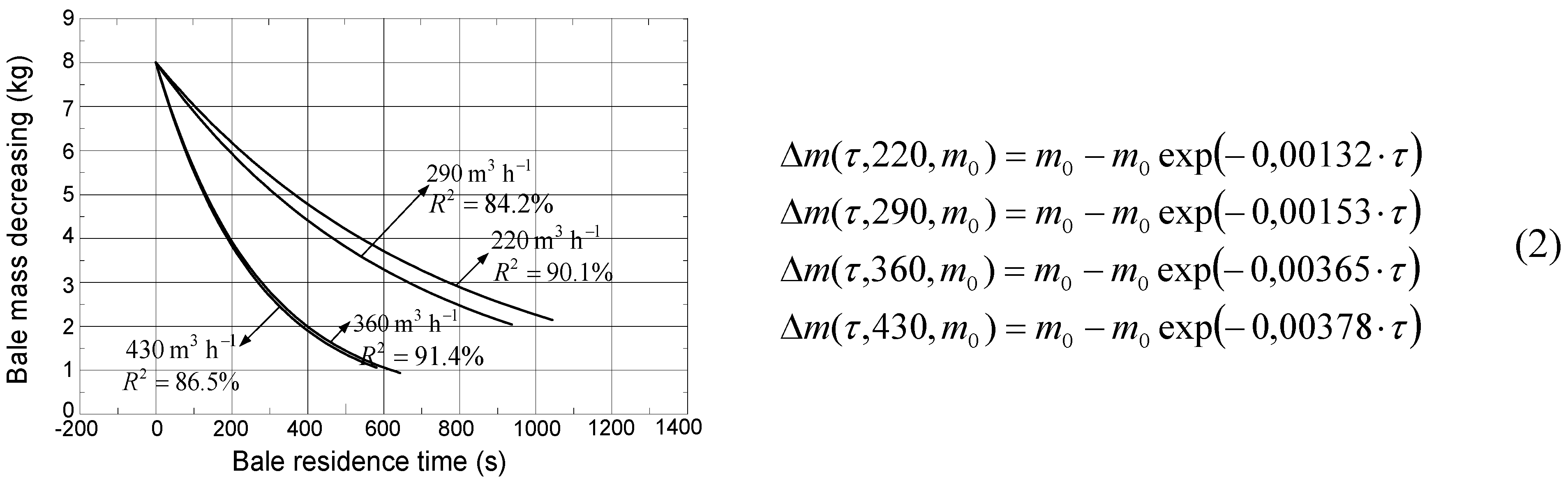
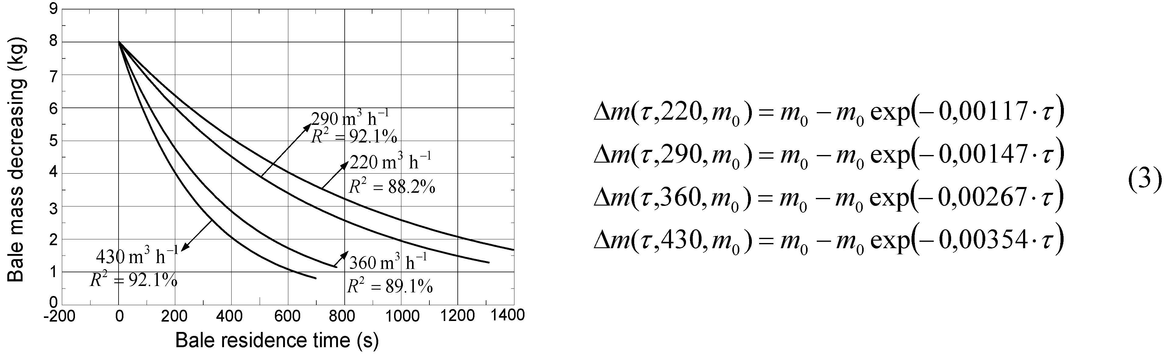
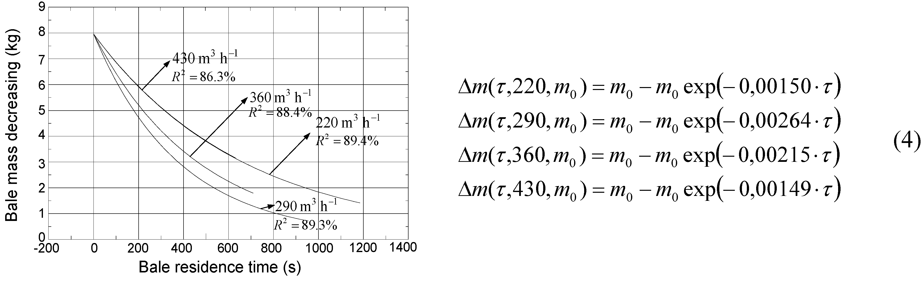
Figure 6,
Figure 7 and
Figure 8 presented graphs of mass loss during the combustion process for each type of regime and recirculation. Furthermore, there are given formulas by which these graphics have been obtained. In Formulas (2–4) unburned bale mass at time
τ for all regimes and all recirculation types is given. In (2–4),
τ is the bale residence time,
m0 is bale weight, Δ
m is a change in bale weight over time.
Figure 6.
Mass loss rate as a function of time, recirculation 0%.
Figure 6.
Mass loss rate as a function of time, recirculation 0%.
Figure 7.
Mass loss rate as a function of time, recirculation 16.5%.
Figure 7.
Mass loss rate as a function of time, recirculation 16.5%.
Figure 8.
Mass loss rate as a function of time, recirculation 33%.
Figure 8.
Mass loss rate as a function of time, recirculation 33%.
If the recirculation is 0 and 16.5% (
Figure 6 and
Figure 7), in the 220 and 290 m
3 h
−1 regimes, bale mass loss is slower, while the time when bale totally burnt is almost twice as long as in the 360 and 430 m
3 h
−1 regimes. These make the 220 and 290 m
3 h
−1 regimes acceptable for further research. If the recirculation of combustion products is 33% (
Figure 8), then bale mass loss is the fastest in the 290 m
3 h
−1 regime, and the slowest in the 430 m
3 h
−1 regime, probably due to an insufficient amount of oxygen. More precisely, disturbance of combustion regimes, due to injection of excessive amounts of air, has been confirmed in several independent studies [
3,
22,
24]. Good combustion requires three preconditions to be satisfied: the presence of the fuel components, mixing with the oxygen fuel components, and heat of activation of the combustion process. Combustion processes in higher operating regimes lead to fast decomposition, so called “dry distillation”, of wheat bales, which suggests that a firebox contains a large amount of combustible components. When the firebox contains substantial amounts of air, then it contains more than enough oxygen for the realization of the combustion process, implying that third basic condition for combustion is not satisfied. This implies the heat of activation of the combustion process is reduced. Large quantities of air, which are inserted in the 430 m
3 h
−1 regime, cool the inside of the firebox and large amounts of heat are removed from the boiler firebox, which further disrupts the combustion process,
i.e., combustion rate decreases. This regime has been picked for a purpose. It serves to certify researches conducted in [
3]. This result is very important, since it clearly points out that, in practice, we cannot count on unlimited power increases of the boiler thermal power due to the addition of air.
3.3. Boiler Energy Efficiency–Experimental Data and Mathematical Model
It is well known that boiler energy efficiency is directly proportional to boiler thermal power and inversely proportional to mass loss. Defining mass loss as a function of bale residence time, allows us to present the boiler energy efficiency rate dependence on bale residence time. The mathematical models which describe those correlations are given in (5a–c) in case of no recirculation, and combustion products recirculation of 16.5 and 33%, respectively.
Here,
b8 and
b9 are the regression coefficients shown in
Table 5a, 5b and 5c for all types of recirculation,
τ is bale residence time,
is air flow,
τkr is the time when the bales were totally burned,
m0 is bale weight, Δ
m is a change in bale weight over time. Note that expressions in the brackets in the numerator in (5a–c) are, according to the second formula in
Section 2.3, boiler thermal power with regression coefficients from
Tables 4a–c.
Table 5.
Estimation of empirical regression coefficients and analysis of variance of model (5a), (a) no recirculation; (b) recirculation 16.5%; (c) recirculation 33%.
Table 5.
Estimation of empirical regression coefficients and analysis of variance of model (5a), (a) no recirculation; (b) recirculation 16.5%; (c) recirculation 33%.
| (a) Level of confidence: 95%, Determination coefficient: R2 = 89.84% |
|---|
| | Estimate | Standard error | t-test | Confidence interval | | | Sum of squares | F-test |
|---|
| b8 * | 0.00649 | 0.00014 | 47.3 | (0.00622, 0.00676) | | Regression | 1,242,130 | 20,011 |
| b9 * | 12.7634 | 1.4589 | 8.7 | (9.8978, 15.6289) | | Residual | 17,256 |
| | | | | | | Total | 1,259,386 |
| (b) Level of confidence: 95%, Determination coefficient: R2 = 95.12% |
| | Estimate | Standard error | t-test | Confidence interval | | | Sum of squares | F-test |
| b8 * | 0.00781 | 0.00008 | 102.8 | (0.00766, 0.00796) | | Regression | 1,585,133 | 57,808 |
| b9 * | 17.9552 | 0.6289 | 28.6 | (16.7201, 19.1904) | | Residual | 8117 |
| | | | | | | Total | 1,593,250 |
| (c) Level of confidence: 95%, Determination coefficient: R2 = 89.02% |
| | Estimate | Standard error | t-test | Confidence interval | | | Sum of squares | F-test |
| b8 * | 0.00649 | 0.00014 | 47.3 | (0.00622, 0.00676) | | Regression | 1,242,130 | 20,011 |
| b9 * | 12.7634 | 1.4588 | 8.7 | (9.8978, 15.6289) | | Residual | 17,256 |
| | | | | | | Total | 1,259,386 |
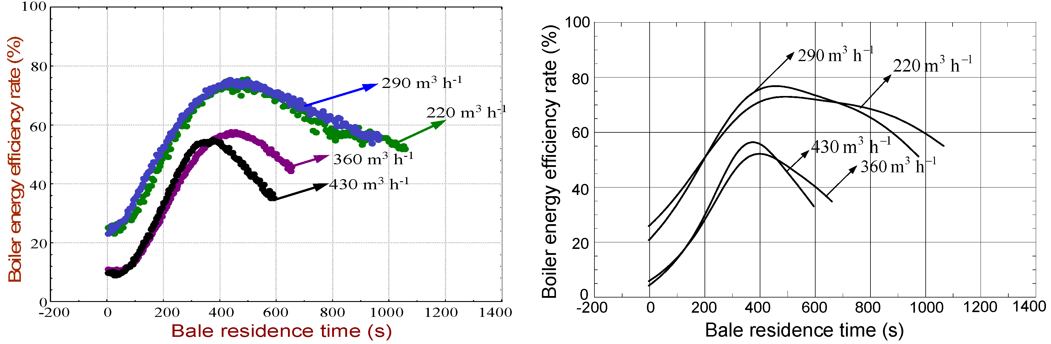
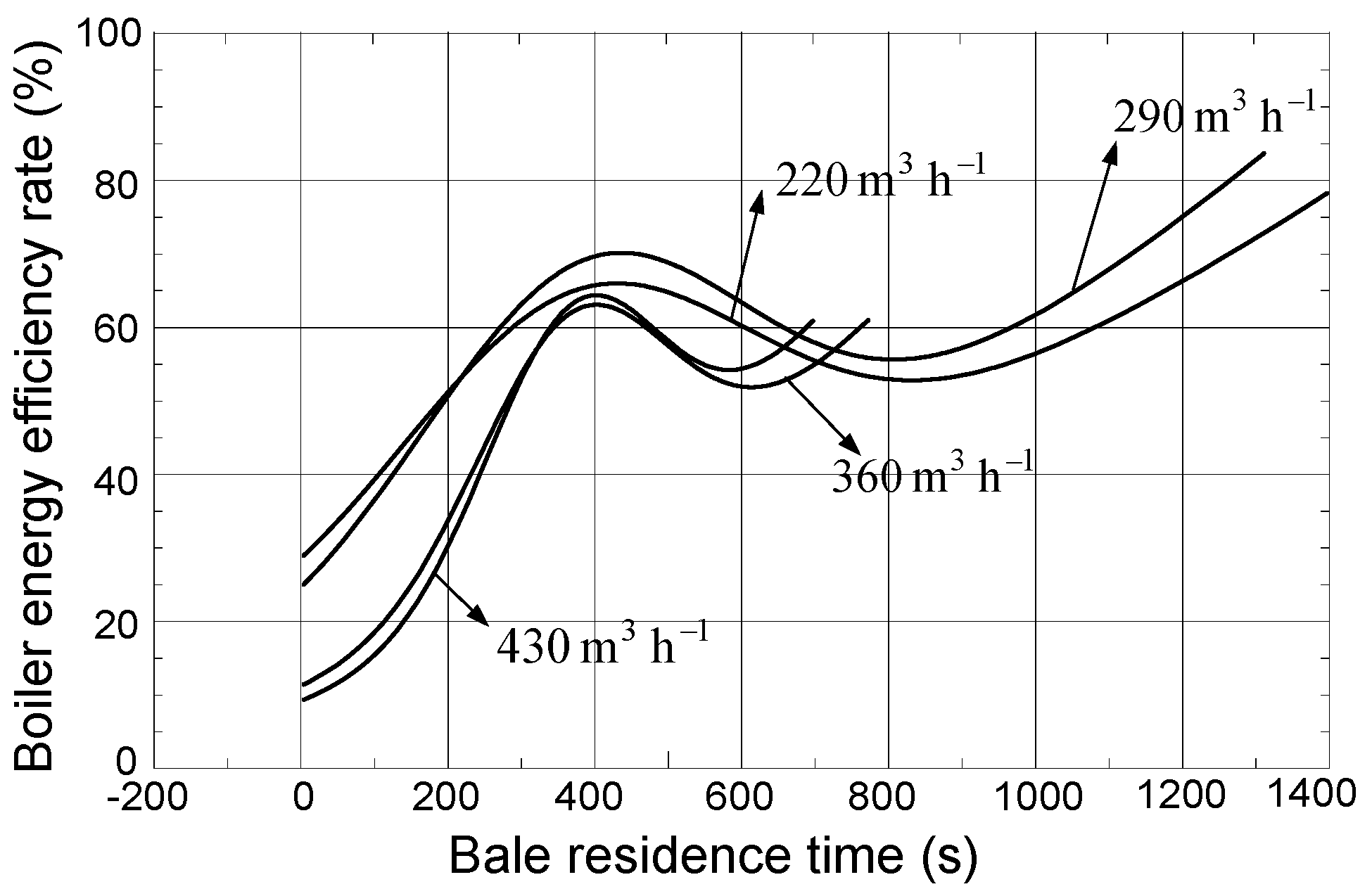
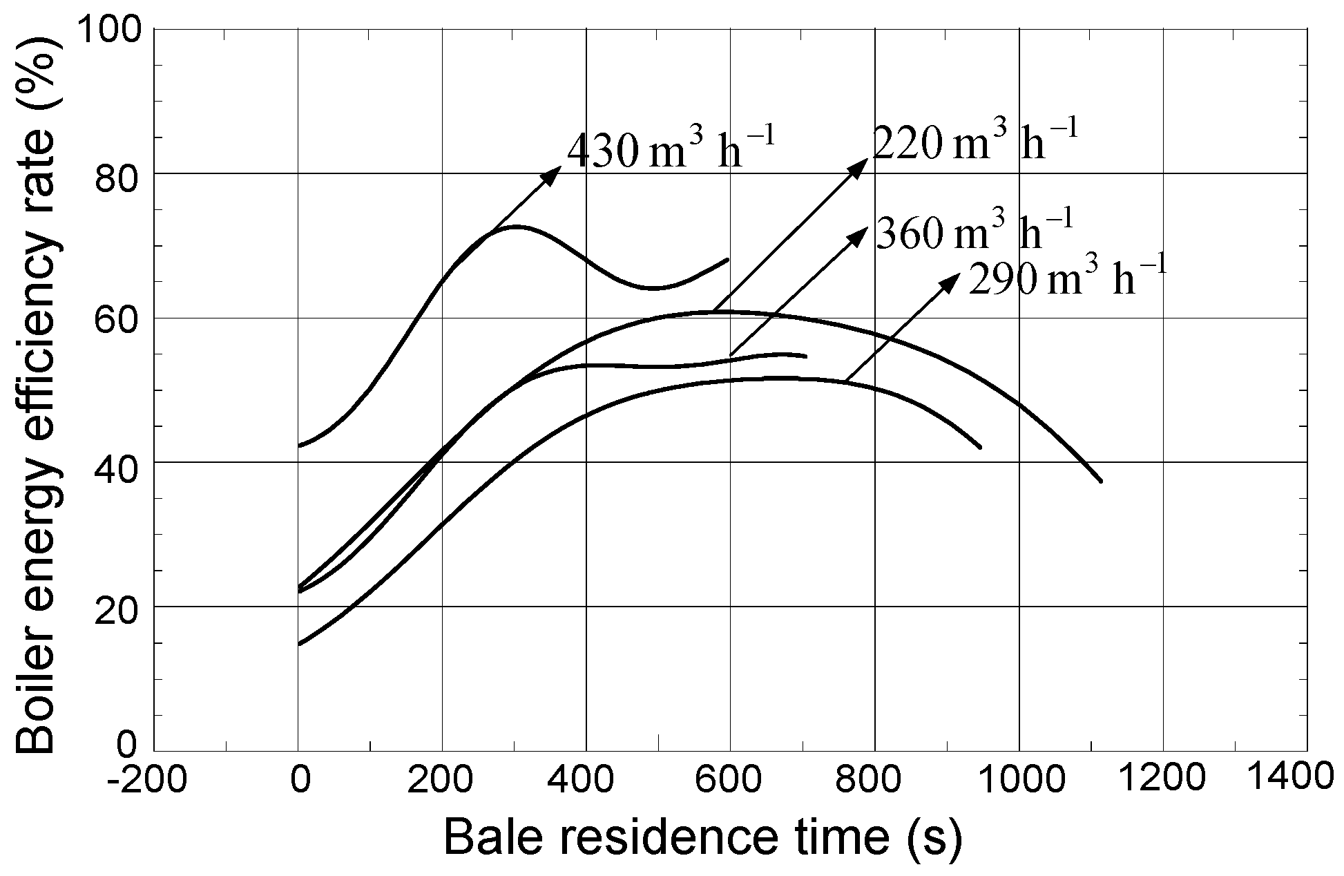
Experimental data of boiler efficiency rate and its graphical interpretation by Formula (5a) is given in
Figure 9(a) and 9(b) (for the case of 0% recirculation), while a graphical interpretation of Formulas (5b) and (5c) is given in
Figure 10 and
Figure 11, respectively.
Figure 9.
(a) Correlation between boiler energy efficiency rate and bale residence time, experimental data, recirculation 0%. (b) Correlation between boiler energy efficiency rate and bale residence time, model (5), recirculation 0%.
Figure 9.
(a) Correlation between boiler energy efficiency rate and bale residence time, experimental data, recirculation 0%. (b) Correlation between boiler energy efficiency rate and bale residence time, model (5), recirculation 0%.
Figure 10.
Correlation between boiler energy efficiency rate and bale residence time, model (6), recirculation 16.5%.
Figure 10.
Correlation between boiler energy efficiency rate and bale residence time, model (6), recirculation 16.5%.
Based on
Figure 9(b) and
Figure 10, one can conclude that the 220 and 290 m
3 h
−1 regimes have the biggest boiler energy efficiency rate in case of 0% and 16.5% recirculation. Together with the previous discussion, this makes the 220 and 290 m
3 h
−1 regimes the optimal ones. If recirculation is 33% (
Figure 11), the biggest boiler energy efficiency rate is in the 430 m
3 h
−1 regime, but now, the bale was completely burned after about 630 seconds. In all other regimes, that time is longer. An increase of combustion product recirculation (in the 220 and 290 m
3 h
−1 regimes) causes a small decrease of boiler energy efficiency.
Based on the above discussion, regarding boiler thermal power, the time when a bale is totally burnt and boiler energy efficiency, two regimes can be taken as optimal ones in case of recirculation of 0 and 16.5% and they are the 220 and 290 m3 h−1 regimes.
Figure 11.
Correlation between boiler energy efficiency rate and bale residence time, model (7), recirculation 33%.
Figure 11.
Correlation between boiler energy efficiency rate and bale residence time, model (7), recirculation 33%.
3.4. Maximum Boiler Thermal Power and Energy Efficiency
To determine compliance between analyzed regimes and nominal boiler power, it is necessary to find out the maximum achieved boiler power as well as maximum boiler efficiency. In
Table 6, the maximum boiler thermal power, corresponding time when the maximum is reached and the energy efficiency of a boiler for all regimes and all types of recirculation are presented.
Table 6.
Maximum boiler thermal power and corresponding boiler energy efficiency rate.
Table 6.
Maximum boiler thermal power and corresponding boiler energy efficiency rate.
| Boiler operating regime | | Recirculation | Boiler operating regime (m3 h−1) |
|---|
| 220 | 290 | 360 | 430 |
|---|
| Time to reach the maximum thermal power and boiler energy and corresponding efficiency rate | τ (s) | 0% | 400 | 388 | 346 | 338 |
| 16.5% | 376 | 373 | 362 | 360 |
| 33% | 434 | 399 | 322 | 286 |
| Pmax (kW) | 0% | 84.05 | 97.97 | 116.96 | 132.19 |
| 16.5% | 68.66 | 84.84 | 112.07 | 133.44 |
| 33% | 68.70 | 83.68 | 89.22 | 101.36 |
| η (%) | 0% | 72.37 | 76.39 | 51.41 | 56.11 |
| 16.5% | 65.77 | 68.89 | 61.81 | 62.71 |
| 33% | 57.79 | 45.77 | 51.01 | 72.47 |
Maximum boiler thermal power (reached in the first half of the combustion process) is less than the nominal one in the 220 and 290 m3 h−1 regimes, which implies that it is enough to have a boiler with a nominal power of 100 kW. In the 430 m3 h−1 regime, maximum boiler thermal power is greater than the nominal one. It follows that this regime is not appropriate for the considered boiler since a thermal power greater than the nominal one can cause damage to a boiler. The corresponding boiler energy efficiency is the greatest (76.39%) in the 290 m3 h−1 regime with 0% recirculation. Note that recirculation of 16.5% decreased maximum boiler thermal power by about 18, 13 and 4% in the 220, 290 and 360 m3 h−1 regimes, respectively.
In
Table 7, maximum boiler energy efficiency, corresponding time when the maximum is reached and boiler thermal power are presented. Among other regimes, in the 290 m
3 h
−1 regime with 0% recirculation, the maximum boiler energy efficiency is reached (almost 80%) in the first half of the combustion process.
Table 7.
Maximum boiler energy efficiency rate and corresponding boiler thermal power.
Table 7.
Maximum boiler energy efficiency rate and corresponding boiler thermal power.
| Boiler operating regime | | Recirculation | Boiler operating regime (m3 h−1) |
|---|
| 220 | 290 | 360 | 430 |
|---|
| Time to reach the maximum boiler energy efficiency rate and corresponding thermal power | τ (s) | 0% | 490 | 454 | 396 | 372 |
| 16.5% | 437 | 433 | 400 | 399 |
| 33% | 595 | 667 | 421 | 497 |
| ηmax (%) | 0% | 74.10 | 77.99 | 53.30 | 57.53 |
| 16.5% | 66.83 | 70.27 | 63.09 | 64.41 |
| 33% | 60.62 | 51.18 | 53.03 | 63.96 |
| P (kW) | 0% | 81.59 | 95.63 | 112.59 | 128.94 |
| 16.5% | 67.57 | 83.23 | 109.73 | 129.95 |
| 33% | 37.90 | 69.01 | 84.05 | 79.62 |
Note that 16.5% recirculation decreased maximum boiler energy efficiency by about 10% in the 220 and 290 m3 h−1 regimes, and increased it by about 18% in the 360 m3 h−1 regime, but this efficiency is still less than one obtained in the 220 and 290 m3 h−1 regimes.
Recirculation of the combustion products is not introduced to reduce emissions of nitrogen oxides from the firebox (although that is partially achieved), but to make the combustion of biomass bales longer, and to affect boiler thermal power and energy efficiency. As it can be seen from
Table 6 and
Table 7, these intentions are partially fulfilled. Regarding
Table 6 and
Table 7, the recirculation in case of low air flow gave significantly worse results in the wheat straw bale combustion process. Lower boiler thermal power was achieved as well as lower boiler energy efficiency. In the case of 16.5% recirculation, with the increase in the total amount of air injected into the firebox, a positive impact of the preheated air on the combustion parameters was achieved, such as s higher maximum boiler thermal power and energy efficiency compared to the case when there is no recirculation. In the case of 33% recirculation, the expected results were not achieved, but in this regime, it can be seen that better indicators of bale burning are also obtained at higher air flow. This can largely be explained by the positive influence of air preheating on combustion of wheat straw bales. From the above discussion, one can conclude that recirculation of 33% is not adequate and should be avoided. Combustion of bales using higher air flow regimes are desirable when recirculation is 16.5%.
All figures in this study, which are obtained by mathematical models, are processed in the package Mathematica 6, which is, as well as package Statistica 10, very applicable in the various problems related to agriculture [
25,
26,
27,
28].
4. Conclusions
Boiler thermal power ranges between 63.47 and 90.90 kW if there is no combustion products recirculation. Boiler thermal power ranges between 57.86 and 88.12 kW with 16.5% recirculation and from 55.65 to 84.98 kW with 33% recirculation. Boiler energy efficiency varies from 36.57 to 60% interval if there is no recirculation,
i.e., from 40.60 to 66.08% if there is 16.5% recirculation (from 41.64 to 49.85% in the case of 33% recirculation). The results point to the fact that the optimal operating regimes are obtained when the air flow through the firebox reaches 220 and 290 m
3 h
−1, if the recirculation is 16.5% and 0%, respectively. Recirculation of 33% causes worse boiler characteristics. These results correspond to the results given in [
21],
i.e., boiler energy efficiency rate ranges between 70 and 80% for smaller boilers which are fed manually with baled biomass.
The presented mathematical models can be perceived as valid for the given boiler plant and the conditions under which the experiments were conducted. The applications of these mathematical models in practice can be multiple. Apart from providing basic information with the aim of improving boiler plant energy efficiency, these mathematical models can be applied in the construction of the future plants, as well as for the reconstruction and mechanization of the existing ones.

 ,
, 

