1. Introduction
At present, the use of wind speed anemometers is increasingly common, their applications having spread from the typical applications in meteorology or in the wind energy industry, to other application in fields affected by the action of wind (e.g., civil engineering structures like moving bridges could need wind speed measurements in order to assure safe operation).
The most used anemometers in scientific or industrial applications are the cups anemometer and propeller anemometer. Both are easy to operate and provide sufficiently accurate wind speed measurements. Today, one of the most (probably the most) important demand of cups and propeller anemometers is represented by the wind energy sector, industry that needs a very accurate wind speed measurements [
1,
2].
The accuracy of an anemometer is assured by its periodic calibration in a wind tunnel [
3]. As a result of this calibration process it is possible to obtain the coefficients A and B of the anemometer’s transfer function:
where
V is the velocity of the flow (wind speed),
f is the anemometer's rotation frequency output, and A (slope) and B (offset) are the calibration coefficients corresponding to the tested anemometer. This linear relationship between the measured wind speed and the anemometer’s output frequency is sufficiently accurate for most purposes [
4].
The present work is part of a more ambitious research program at the IDR/UPM Institute to review and analyze large series of anemometers’ calibrations. In a previous study [
3], based on series of calibrations from January 2003 to August 2007, the influence of the wind speed range and some anemometer geometrical parameters on the calibrations results was studied. In a second analysis campaign, the deviation over time of cup anemometer calibrations results from initial values was studied. The aforementioned period of series of calibrations was extended to January 2001 and January 2011 in order to obtain statistically more significant results. Based on the changes observed in the calibration constants over time and their effect on the wind speed measurements (and subsequently, on AEP), a recalibration schedule was proposed for anemometers not used in the field (just stored). No clear evolution of the calibration constants with time elapsed after the first calibration was observed with regard to anemometers used in field (and therefore used in long periods of time under different and variable ambient conditions). The results concerning these anemometers used in field showed a high scattering level, mainly due to the different ambient conditions during the time of service. This was observed even in anemometers that were not subjected to severe maintenance (change of bearings, change of electronics, change of cups rotor) during long periods of time.
In this third step, the influence of the environmental conditions during the calibration process on the calibration constants A and B have been analyzed. Ambient conditions, especially changes in air density from the value at sea level (
ρ = 1.225 kg·m
−3), are taken into account in the IEC 61400-1 International Standard [
5] with respect to the wind mills power curve measurement and AEP estimations. More specifically and regarding the anemometers’ behavior, in the IEC 61400-12-1 International Standard [
6] the air density, ranging from
ρ = 0.9 kg·m
−3 to
ρ = 1.3 kg·m
−3, is defined as an influence parameter for anemometer classification. The importance of taking into account changes in air density must be underlined, as wind energy production estimations depend linearly on this parameter.
Ambient conditions do have an effect on the anemometers’ behavior, as their response (changes in the rotational velocity,
ω) depends on the aerodynamic and frictional torques (
QA and
Qf respectively), that is:
where
I is the moment of inertia. The aerodynamic torque,
QA, is a function of the air density,
ρ, among other parameters, and the frictional torque,
Qf, is a function of the ambient temperature,
T, and the rotational velocity,
ω [
6].
In a previous study carried out at the IDR/UPM Institute in 2003 over a large series of NRG Maximum 40 cup anemometers [
7], the effect of the air density on the transfer function constants was analyzed. A linear behavior as a function of the density was observed. However, the effect of the air density variations on the anemometers performance was considered minor as “In all cases the dependency versus density, humidity and test equipment reveals variation in
f7m/s less than 1% for homogenized anemometer groups, therefore lower than deviation allowed in MEASNET procedures” (
f7m/s stands for the anemometer’s output frequency at 7 m s
−1 wind speed).
The aim of the present study was to analyze the calibration results of different anemometer models as a function of the air density, in order to estimate the errors of the measured wind speed due to changes in the environmental conditions (temperature, pressure and humidity) from the ones at which the anemometer was initially calibrated, and their effect on AEP estimations.
2. Testing Configuration and Anemometers Studied
At the IDR/UPM Institute, anemometer calibrations are performed in the S4 wind tunnel. This facility is an open-circuit wind tunnel with a closed test section measuring 0.9 by 0.9 m. It is served by four 7.5 kW fans with a flow uniformity better than 0.2% in the testing area. More details concerning the facility and the calibration process are included in reference [
3]. The calibrations analyzed in the present paper were performed following the MEASNET recommendations (over 13 points and 4 to 16 m s
−1). The statistical uncertainty is calculated for each calibration using the procedure described by MEASNET [
8] (see also References [
6] and [
9]).
Nine different cup anemometer models and a propeller one were studied: Thies Clima 4.3350, 4.3351 and 4.3303 (Thies Clima: Göttingen, Germany); Vector Instruments A100 L2 and A100 LK (Windspeed Limited, trading as Vector Instruments: Rhyl, UK); Ornytion 107A (Ornytion: Bergondo, A Coruña, Spain); RM Young 05103 and 3002/3102 (R. M. Young Company: Traverse City, MI, USA); Secondwind C3 (Secondwind: Somerville, MA, USA); and NRG Systems 40/40C (NRG Systems, Inc: Hinesburg, VT, USA). A list of the anemometer models studied are included in
Table 1, together with the number of calibrations analyzed and the period of time in which these calibrations where performed. More detailed information with regard to the geometrical and other characteristics of these anemometers can be found in reference [
3]. Only anemometer models that were calibrated at least 150 times at the IDR/UPM from March 2003 to February 2011 were considered in the present work, in order to have statistically more significant results. The data concerning the calibrations performed on the three anemometers used at the IDR/UPM Institute for internal procedures (Vector Instruments A100 L2, Thies Clima 4.3350, and Climatronics 100075 (Climatronics Corp.: Bohemia, NY, USA)) was also analyzed (see
Table 1).
Table 1.
Anemometer models studied, number of calibration performed, and the period of time in which these calibrations were performed.
Table 1.
Anemometer models studied, number of calibration performed, and the period of time in which these calibrations were performed.
| Anemometer | Calibrations | From | To |
| NRG Systems Maximum 40/40C | 1945 | 27/05/2003 | 20/01/2011 |
| Secondwind C3 | 172 | 05/12/2007 | 16/02/2011 |
| Thies Clima 4.3350 | 2790 | 25/11/2003 | 15/02/2011 |
| Thies Clima 4.3351 | 894 | 03/12/2009 | 22/02/2011 |
| Thies Clima 4.3303 | 323 | 11/09/2003 | 09/09/2010 |
| Vector Instruments A100 L2 | 327 | 30/04/2003 | 05/01/2011 |
| Vector Instruments A100 LK | 656 | 22/03/2005 | 16/02/2011 |
| Ornytion 107A | 772 | 11/05/2004 | 11/02/2011 |
| RM Young 3002/3102 | 199 | 31/03/2003 | 15/11/2010 |
| RM Young 05103 | 266 | 02/11/2004 | 08/02/2011 |
| IDR/UPM Anemometers | Calibrations | From | To |
| Climatronics 100075 | 64 | 30/01/2001 | 28/06/2006 |
| Vector Instruments A100 L2 | 70 | 10/09/2003 | 30/10/2007 |
| Thies Clima 4.3350 | 176 | 05/10/2006 | 17/02/2011 |
Following MEASNET procedures, all calibrations performed at the IDR/UPM include a measurement of the ambient conditions (air temperature, pressure and air humidity). In
Figure 1, the values of the mentioned ambient conditions, measured during the calibrations performed on the three IDR/UPM anemometers are shown together with the air density calculated using those values (see References [
6], [
8] and [
10]). In the mentioned figure the seasonal variations of the ambient conditions, especially the temperature, can be observed. The ambient conditions in which those calibrations were carried out are in the following brackets, temperature: from 19.2 °C to 32.3 °C; pressure: from 920.20 HPa to 959.37 HPa; humidity: from 16.5% to 50.6%. Finally, the air density calculated from these data varied from 1.068 kg·m
−3 to 1.128 kg·m
−3.
3. Results and Discussion
In
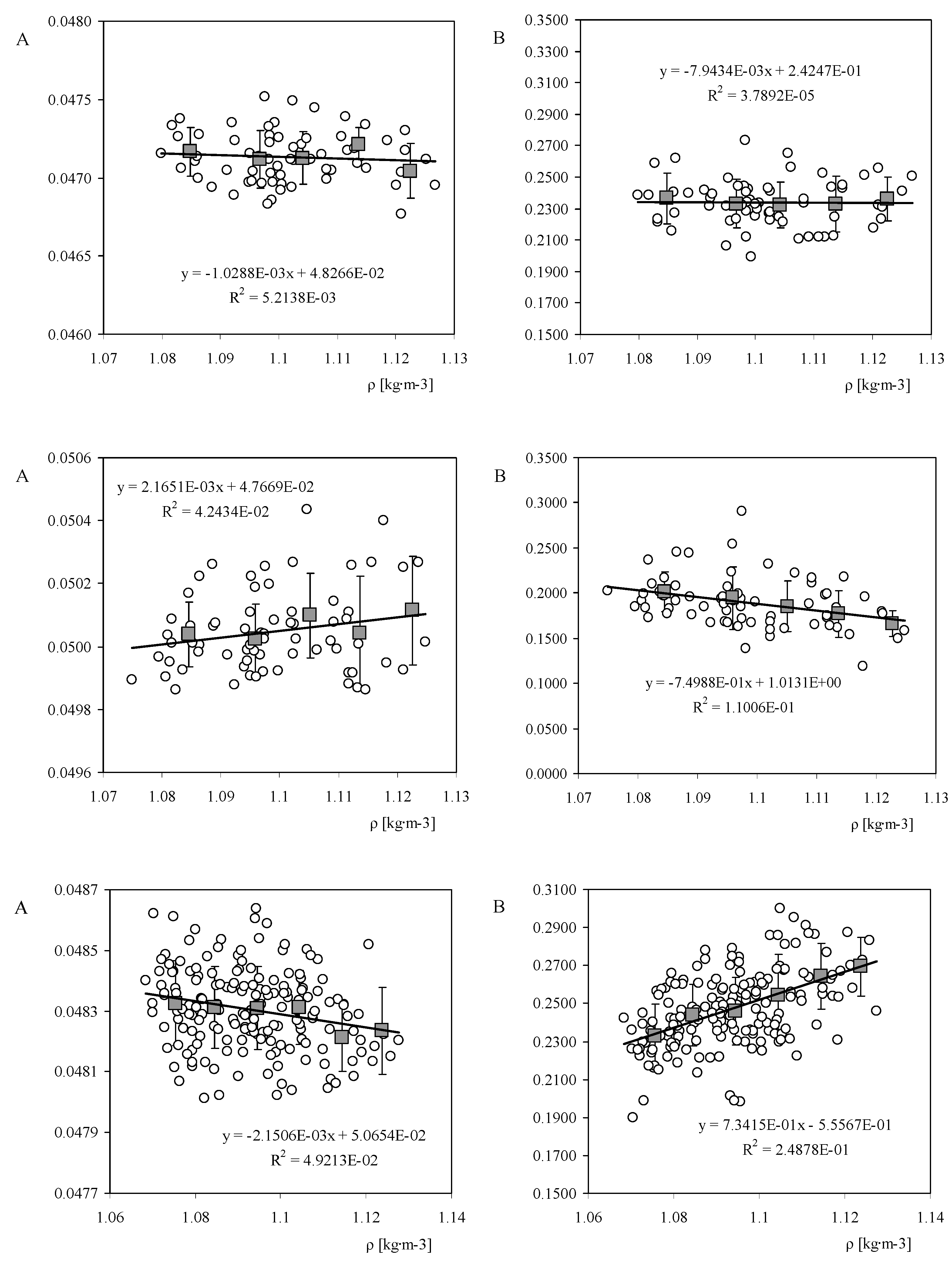
Figure 2 the values of calibration constants A and B of the three IDR/UPM anemometers as a function of the air density value during each calibration are shown. The linear fit has been added to the graphs, together with the moving average points and the standard deviation bars calculated for ∆
ρ= 0.01 kg·m
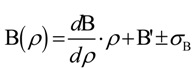
−3 density brackets. In all cases there seems to be a linear behavior as a function of the air density, with regard to both calibration coefficients. If this linear behavior is considered, calibration constants can be expressed as:
where
dA/
dρ,
dB/
dρ, A’ and B’ are the constants of the linear fittings to the data, and
σA and
σB are standard deviations of the mentioned data. Assuming a Gaussian process, with these Equations the constants of the anemometer’s transfer function can be estimated as a function of the air density with 68.2% confidence level. See in
Table 2 the values of the linear fittings coefficients (values of
dA/
dρ,
dB/
dρ, A’ and B’) corresponding to the data shown in the
Figure 2. See also in
Table 3 the moving average and standard deviation values with regard to these anemometers (as said, these values are calculated for ∆
ρ = 0.01 kg·m
−3 density brackets).
Table 2.
Linear fitting coefficients (that is, values of the slopes:
dA/
dρ and
dB/
dρ; and offsets: A’ and B’ of the linear fittings), correspondent to the measured calibration constants, A and B of the IDR/UPM Institute anemometers shown as a function of the air density (see also
Figure 2).
Table 2.
Linear fitting coefficients (that is, values of the slopes: dA/dρ and dB/dρ; and offsets: A’ and B’ of the linear fittings), correspondent to the measured calibration constants, A and B of the IDR/UPM Institute anemometers shown as a function of the air density (see also Figure 2).
| IDR/UPM Anemometers | dA/dρ | A’ | dB/dρ | B’ |
|---|
| Climatronics 100075 | −1.0288 × 10⁻³ | 4.8266 × 10⁻² | −7.9434 × 10⁻³ | 2.4247 × 10⁻¹ |
| Vector Instruments A100 L2 | 2.1651 × 10⁻³ | 4.7669 × 10⁻² | −7.4988 × 10⁻¹ | 1.0131 |
| Thies Clima 4.3350 | −2.1506 × 10⁻³ | 5.0654 × 10⁻² | 7.3415 × 10⁻¹ | −5.5567 × 10⁻¹ |
Table 3.
Moving average and standard deviation values correspondent to the calibration constants of the three IDR/UPM anemometers devoted to the internal procedures, as a function of the air density,
ρ, during calibrations (see also
Figure 2).
Table 3.
Moving average and standard deviation values correspondent to the calibration constants of the three IDR/UPM anemometers devoted to the internal procedures, as a function of the air density, ρ, during calibrations (see also Figure 2).
| Climatronics 100075 |
| Density brackets, ρ [kg·m−3] | A | σA | B | σB |
| 1.08–1.09 | 4.7165 × 10⁻² | 1.5283 × 10⁻⁴ | 2.3641 × 10⁻¹ | 1.6140 × 10⁻² |
| 1.09–1.10 | 4.7118 × 10⁻² | 1.8149 × 10⁻⁴ | 2.3302 × 10⁻¹ | 1.5425 × 10⁻² |
| 1.10–1.11 | 4.7127 × 10⁻² | 1.6599 × 10⁻⁴ | 2.3231 × 10⁻¹ | 1.4357 × 10⁻² |
| 1.11–1.12 | 4.7215 × 10⁻² | 1.0677 × 10⁻⁴ | 2.3297 × 10⁻¹ | 1.7513 × 10⁻² |
| 1.12–1.13 | 4.7043 × 10⁻² | 1.7449 × 10⁻⁴ | 2.3596 × 10⁻¹ | 1.3773 × 10⁻² |
| Vector Instruments 100 L2 |
| Density brackets, ρ [kg·m−3] | A | σA | B | σB |
| 1.08–1.09 | 5.0039 × 10⁻² | 1.0304 × 10⁻⁴ | 2.0155 × 10⁻¹ | 2.2062 × 10⁻² |
| 1.09–1.10 | 5.0026 × 10⁻² | 1.1063 × 10⁻⁴ | 1.9446 × 10⁻¹ | 3.4967 × 10⁻² |
| 1.10–1.11 | 5.0099 × 10⁻² | 1.3356 × 10⁻⁴ | 1.8518 × 10⁻¹ | 2.7921 × 10⁻² |
| 1.11–1.12 | 5.0044 × 10⁻² | 1.8094 × 10⁻⁴ | 1.7716 × 10⁻¹ | 2.5901 × 10⁻² |
| 1.12–1.13 | 5.0114 × 10⁻² | 1.7130 × 10⁻⁴ | 1.6621 × 10⁻¹ | 1.4449 × 10⁻² |
| Thies Clima 4.3350 |
| Density brackets, ρ [kg·m−3] | A | σA | B | σB |
| 1.07–1.08 | 4.8326 × 10⁻² | 1.3928 × 10⁻⁴ | 2.3289 × 10⁻¹ | 1.6668 × 10⁻² |
| 1.08–1.09 | 4.8313 × 10⁻² | 1.3413 × 10⁻⁴ | 2.4384 × 10⁻¹ | 1.6079 × 10⁻² |
| 1.09–1.10 | 4.8309 × 10⁻² | 1.3651 × 10⁻⁴ | 2.4586 × 10⁻¹ | 1.7911 × 10⁻² |
| 1.10–1.11 | 4.8311 × 10⁻² | 1.2106 × 10⁻⁴ | 2.5431 × 10⁻¹ | 2.1532 × 10⁻² |
| 1.11–1.12 | 4.8214 × 10⁻² | 1.1276 × 10⁻⁴ | 2.6434 × 10⁻¹ | 1.7122 × 10⁻² |
| 1.12–1.13 | 4.8235 × 10⁻² | 1.4268 × 10⁻⁴ | 2.6958 × 10⁻¹ | 1.5478 × 10⁻² |
Figure 1.
Ambient conditions and air density during calibrations performed to the IDR/UPM Institute anemometers: Climatronics 100075 (squares), Vector instruments A100 L2 (circles), and Thies Clima 4.3350 (triangles), from January 2001 to February 2011.
Figure 1.
Ambient conditions and air density during calibrations performed to the IDR/UPM Institute anemometers: Climatronics 100075 (squares), Vector instruments A100 L2 (circles), and Thies Clima 4.3350 (triangles), from January 2001 to February 2011.
Figure 2.
Calibration constants,
A and
B, with regard to the IDR/UPM Institute Climatronics 100075 (
top), Vector Instruments A100 L2 (
middle), and Thies Clima 4.3350 (
bottom) anemometers as a function of the air density value,
ρ, during the calibrations. The linear fit to the data has been included in the graphs. The grey squares represent the moving average values (see also
Table 2).
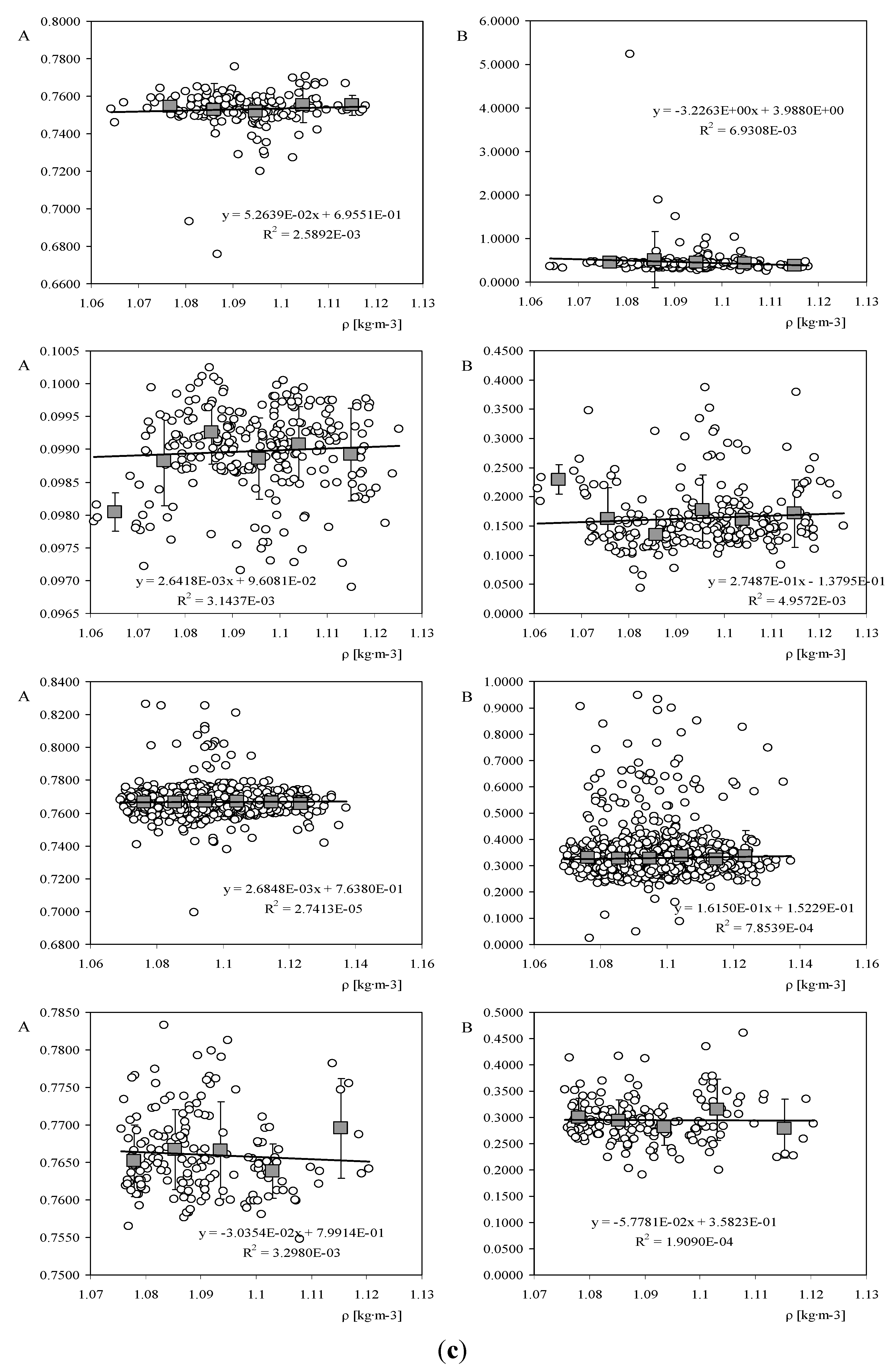
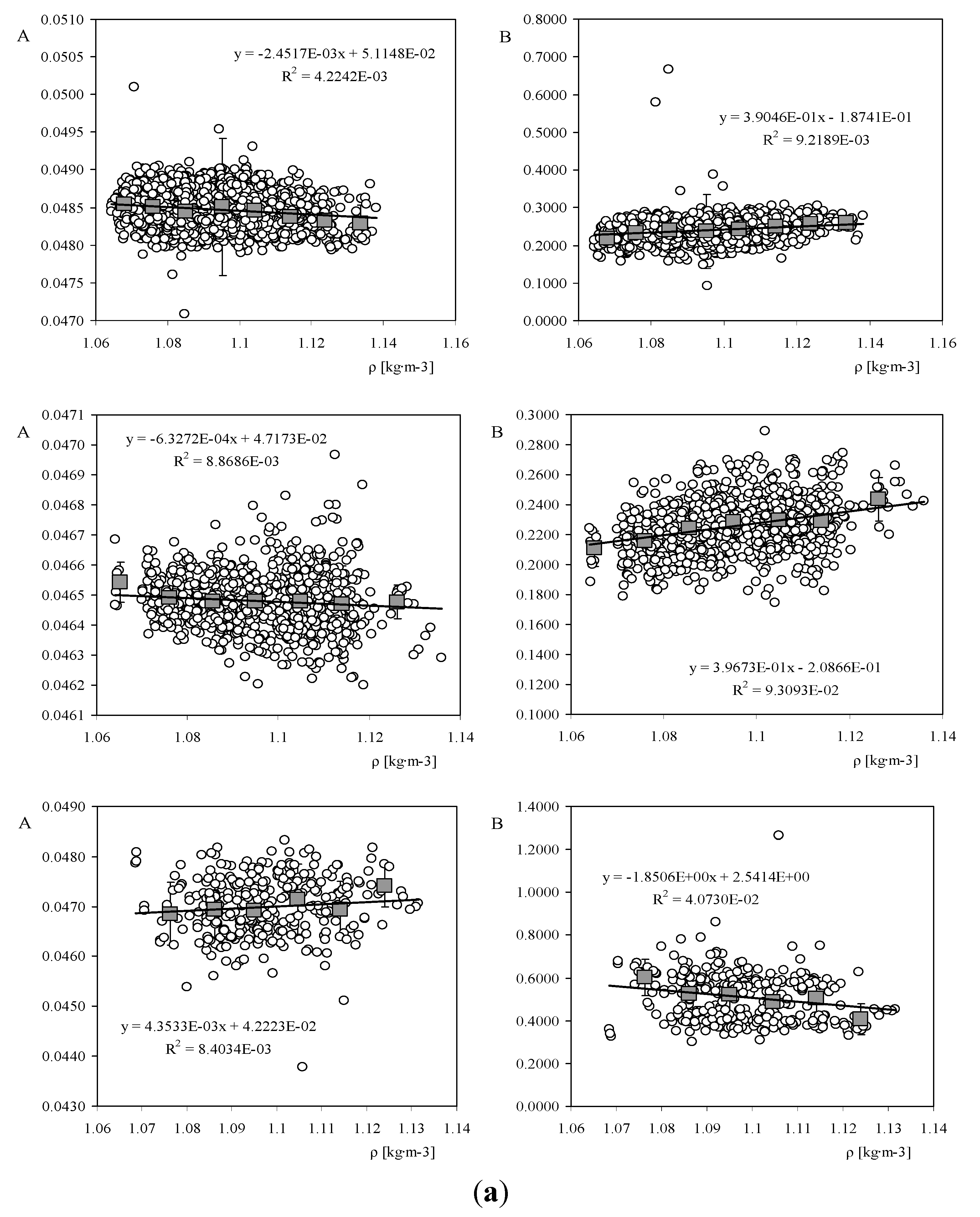
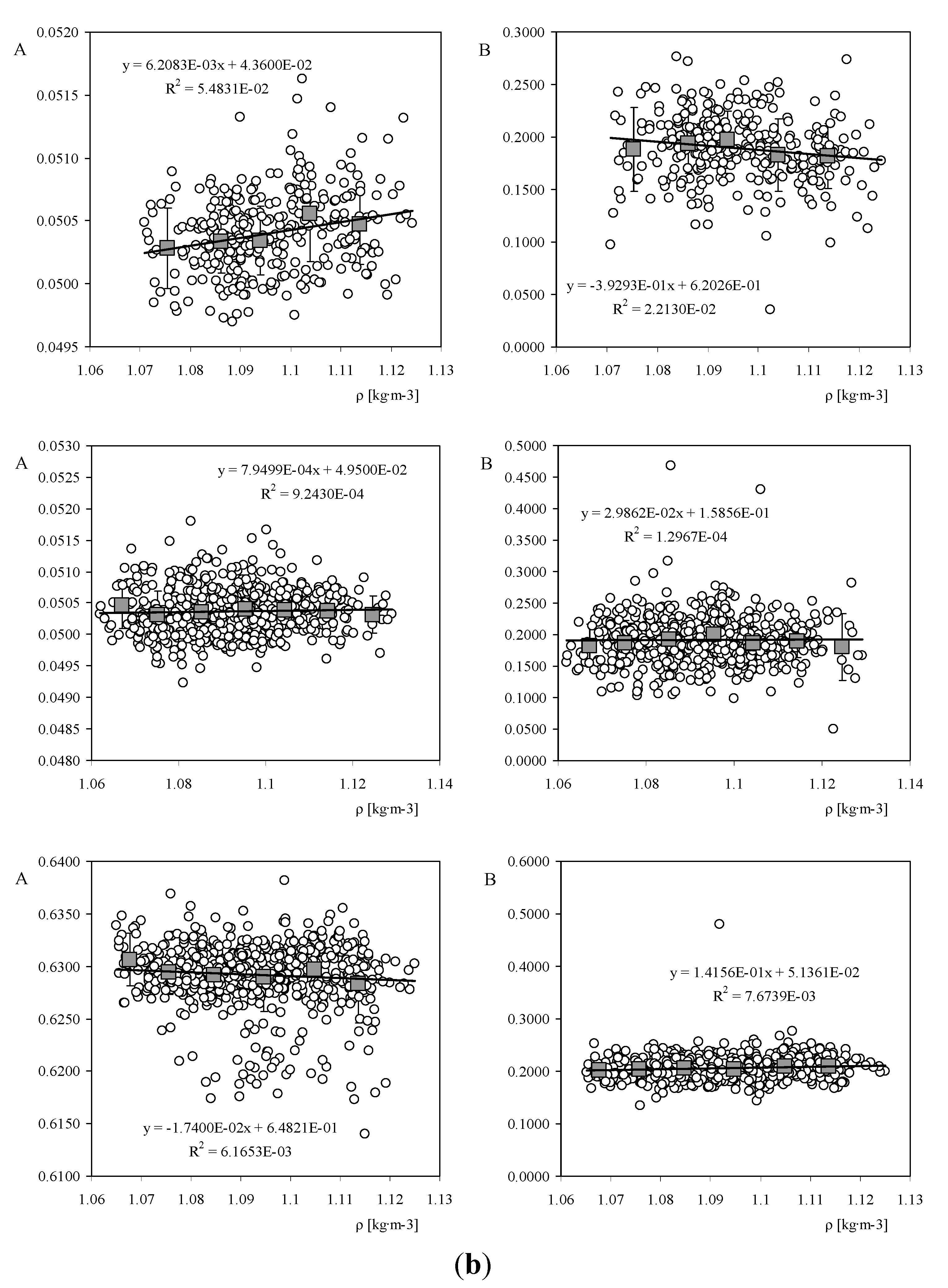
In
Figure 3a–c the variation with air density of calibration constants A and B of the anemometer models studied is shown. Each point of the graphs in these figures represents the first calibration of a single anemometer. The linear fit and the moving average values, together with the standard deviation bars (calculated for ∆
ρ = 0.01 kg·m
−3 density brackets), have also been included in each graph. In
Table 4 the values of the coefficients with regard to the mentioned linear fittings are included for all the anemometer models studied.
Figure 3.
(
a) Calibration constants,
A and
B, with regard to the Thies Clima 4.3350 (
top), 4.3351 (
middle), and 4.3303 (
bottom) anemometer models tested at IDR/UPM Institute, as a function of the air density value,
ρ, during the calibrations. The linear fit to the data has been included in the graphs. The grey squares represent the moving average values (see also
Table 5); (
b) Calibration constants,
A and
B, with regard to the Vector Instruments A100 L2 (
top), Vector Instruments A100 LK (middle), and Ornytion 107A (
bottom) anemometer models tested at IDR/UPM Institute, as a function of the air density value,
ρ, during the calibrations. The linear fit to the data has been included in the graphs. The grey squares represent the moving average values (see also
Table 5); (
c) Calibration constants, A and B, with regard to the RM Young 3002–3102 (
top) and 05103 (
middle-top), NRG System 40/40C (
middle-bottom), and Secondwind C3 (
bottom) anemometer models tested at IDR/UPM Institute, as a function of the air density value,
ρ, during the calibrations. The linear fit to the data has been included in the graphs. The grey squares represent the moving average values (see also
Table 5).
The values of the moving average and standard deviation values are included for each density bracket in
Table 5a–c. As in the case of the three single individual anemometers studied, the calibration constants corresponding to a group of different anemometers of the same model also seem to have a linear behavior as a function of the air density, therefore, Equations (3) and (4) could also be used to describe the effect of air density changes on the transfer function of the anemometer models considered.
Table 4.
Linear fitting coefficients (values of
dA/
dρ,
dB/
dρ, A’ and B’), correspondent to the measured calibration constants, A and B of the anemometer models studied shown as a function of the air density (see also
Figure 3a–c).
Table 4.
Linear fitting coefficients (values of dA/dρ, dB/dρ, A’ and B’), correspondent to the measured calibration constants, A and B of the anemometer models studied shown as a function of the air density (see also Figure 3a–c).
| Anemometers | dA/dρ | A’ | dB/dρ | B’ |
|---|
| NRG Systems Maximum 40/40C | 2.6848 × 10⁻³ | 7.6380 × 10⁻¹ | 1.6150 × 10⁻¹ | 1.5229 × 10⁻¹ |
| Secondwind C3 | −3.0354 × 10⁻² | 7.9914 × 10⁻¹ | −5.7781 × 10⁻² | 3.5823 × 10⁻¹ |
| Thies Clima 4.3350 | −2.4517 × 10⁻³ | 5.1148 × 10⁻² | 3.9046 × 10⁻¹ | −1.8741 × 10⁻¹ |
| Thies Clima 4.3351 | −6.3272 × 10⁻⁴ | 4.7173 × 10⁻² | 3.9673 × 10⁻¹ | −2.0866 × 10⁻¹ |
| Thies Clima 4.3303 | 4.3533 × 10⁻³ | 4.2223 × 10⁻² | −1.8506 | 2.5414 |
| Vector Instruments A100 L2 | 6.2083 × 10⁻³ | 4.3600 × 10⁻² | −3.9293 × 10⁻¹ | 6.2026 × 10⁻¹ |
| Vector Instruments A100 LK | 7.9499 × 10⁻⁴ | 4.9500 × 10⁻² | 2.9862 × 10⁻² | 1.5856 × 10⁻¹ |
| Ornytion 107A | −1.7400 × 10⁻² | 6.4821 × 10⁻¹ | 1.4156 × 10⁻¹ | 5.1361 × 10⁻² |
| RM Young 3002/3102 | 5.2639 × 10⁻² | 6.9551 × 10⁻¹ | −3.2263 | 3.9880 |
| RM Young 05103 | 2.6418 × 10⁻³ | 9.6081 × 10⁻² | 2.7487 × 10⁻¹ | −1.3795 × 10⁻¹ |
Table 5.
(
a–c) Values of the moving average and standard deviation with regard to the calibration constants of the analyzed anemometers’ models as a function of the air density,
ρ, during calibrations (see also
Figure 3a–c).
(a)
| Vector Instruments 100 L2 |
| Density brackets, ρ [kg·m−3] | A | σA | B | σB |
| 1.07–1.08 | 5.0283 × 10⁻² | 3.2191 × 10⁻⁴ | 1.8799 × 10⁻¹ | 4.0095 × 10⁻² |
| 1.08–1.09 | 5.0337 × 10⁻² | 2.5329 × 10⁻⁴ | 1.9383 × 10⁻¹ | 2.8434 × 10⁻² |
| 1.09–1.10 | 5.0343 × 10⁻² | 2.7259 × 10⁻⁴ | 1.9715 × 10⁻¹ | 2.7380 × 10⁻² |
| 1.10–1.11 | 5.0554 × 10⁻² | 3.7527 × 10⁻⁴ | 1.8254 × 10⁻¹ | 3.4322 × 10⁻² |
| 1.11–1.12 | 5.0472 × 10⁻² | 3.1500 × 10⁻⁴ | 1.8174 × 10⁻¹ | 3.1234 × 10⁻² |
| Vector Instruments 100 LK |
| Density brackets, ρ [kg·m−3] | A | σA | B | σB |
| 1.06–1.07 | 5.0467 × 10⁻² | 3.7453 × 10⁻⁴ | 1.8222 × 10⁻¹ | 3.4140 × 10⁻² |
| 1.07–1.08 | 5.0304 × 10⁻² | 3.8950 × 10⁻⁴ | 1.8694 × 10⁻¹ | 3.5435 × 10⁻² |
| 1.08–1.09 | 5.0359 × 10⁻² | 4.0522 × 10⁻⁴ | 1.9201 × 10⁻¹ | 4.0930 × 10⁻² |
| 1.09–1.10 | 5.0394 × 10⁻² | 3.5665 × 10⁻⁴ | 1.9953 × 10⁻¹ | 3.2565 × 10⁻² |
| 1.10–1.11 | 5.0384 × 10⁻² | 3.0863 × 10⁻⁴ | 1.8628 × 10⁻¹ | 3.4949 × 10⁻² |
| 1.11–1.12 | 5.0370 × 10⁻² | 2.8924 × 10⁻⁴ | 1.8986 × 10⁻¹ | 2.6092 × 10⁻² |
| 1.12–1.13 | 5.0316 × 10⁻² | 3.0112 × 10⁻⁴ | 1.7981 × 10⁻¹ | 5.3004 × 10⁻² |
| Thies Clima 4.3350 |
| Density brackets, ρ [kg·m−3] | A | σA | B | σB |
| 1.06–1.07 | 4.8538 × 10⁻² | 1.8688 × 10⁻⁴ | 2.1897 × 10⁻¹ | 1.9390 × 10⁻² |
| 1.07–1.08 | 4.8509 × 10⁻² | 2.4489 × 10⁻⁴ | 2.3322 × 10⁻¹ | 2.0901 × 10⁻² |
| 1.08–1.09 | 4.8450 × 10⁻² | 2.4316 × 10⁻⁴ | 2.3964 × 10⁻¹ | 2.9167 × 10⁻² |
| 1.09–1.10 | 4.8508 × 10⁻² | 9.1022 × 10⁻⁴ | 2.3693 × 10⁻¹ | 9.8647 × 10⁻² |
| 1.10–1.11 | 4.8461 × 10⁻² | 2.3200 × 10⁻⁴ | 2.4343 × 10⁻¹ | 2.3354 × 10⁻² |
| 1.11–1.12 | 4.8375 × 10⁻² | 1.9879 × 10⁻⁴ | 2.4867 × 10⁻¹ | 1.8413 × 10⁻² |
| 1.12–1.13 | 4.8320 × 10⁻² | 2.2199 × 10⁻⁴ | 2.5738 × 10⁻¹ | 2.0725 × 10⁻² |
| 1.13–1.14 | 4.8283 × 10⁻² | 2.5340 × 10⁻⁴ | 2.5836 × 10⁻¹ | 1.7769 × 10⁻² |
| Thies Clima 4.3351 |
| Density brackets, ρ [kg·m−3] | A | σA | B | σB |
| 1.06–1.07 | 4.6543 × 10⁻² | 6.6424 × 10⁻⁵ | 2.1065 × 10⁻¹ | 1.2032 × 10⁻² |
| 1.07–1.08 | 4.6492 × 10⁻² | 7.0657 × 10⁻⁵ | 2.1546 × 10⁻¹ | 1.5348 × 10⁻² |
| 1.08–1.09 | 4.6480 × 10⁻² | 7.5682 × 10⁻⁵ | 2.2403 × 10⁻¹ | 1.6510 × 10⁻² |
| 1.09–1.10 | 4.6478 × 10⁻² | 9.5766 × 10⁻⁵ | 2.2840× 10⁻¹ | 1.7593 × 10⁻² |
| 1.10–1.11 | 4.6477 × 10⁻² | 1.0256 × 10⁻⁴ | 2.2980 × 10⁻¹ | 1.9027 × 10⁻² |
| 1.11–1.12 | 4.6471 × 10⁻² | 1.2506 × 10⁻⁴ | 2.2903 × 10⁻¹ | 1.9003 × 10⁻² |
| 1.12–1.13 | 4.6477 × 10⁻² | 5.7246 × 10⁻⁵ | 2.4383 × 10⁻¹ | 1.4527 × 10⁻² |
(b)
| Thies Clima 4.3303 |
| Density brackets, ρ [kg·m−3] | A | σA | B | σB |
| 1.07–1.08 | 4.6857 × 10⁻² | 6.2541 × 10⁻⁴ | 6.0287 × 10⁻¹ | 8.4150 × 10⁻² |
| 1.08–1.09 | 4.6933 × 10⁻² | 5.6513 × 10⁻⁴ | 5.2722 × 10⁻¹ | 1.0864 × 10⁻¹ |
| 1.09–1.10 | 4.6912 × 10⁻² | 5.4037 × 10⁻⁴ | 5.1972 × 10⁻¹ | 1.1003 × 10⁻¹ |
| 1.10–1.11 | 4.7149 × 10⁻² | 6.9398 × 10⁻⁴ | 4.8698 × 10⁻¹ | 1.3379 × 10⁻¹ |
| 1.11–1.12 | 4.6941 × 10⁻² | 5.7003 × 10⁻⁴ | 5.0679 × 10⁻¹ | 9.7130 × 10⁻² |
| 1.12–1.13 | 4.7414 × 10⁻² | 4.1312 × 10⁻⁴ | 4.0761 × 10⁻¹ | 7.1281 × 10⁻² |
| Secondwind C3 |
| Density brackets, ρ [kg·m−3] | A | σA | B | σB |
| 1.07–1.08 | 7.6525 × 10⁻¹ | 4.7890 × 10⁻³ | 3.0062 × 10⁻¹ | 3.5492 × 10⁻² |
| 1.08–1.09 | 7.6671 × 10⁻¹ | 5.2839 × 10⁻³ | 2.9418 × 10⁻¹ | 3.9042 × 10⁻² |
| 1.09–1.10 | 7.6664 × 10⁻¹ | 6.4810 × 10⁻³ | 2.8178 × 10⁻¹ | 3.4694 × 10⁻² |
| 1.10–1.11 | 7.6383 × 10⁻¹ | 3.6591 × 10⁻³ | 3.1452 × 10⁻¹ | 5.7803 × 10⁻² |
| 1.11–1.12 | 7.6953 × 10⁻¹ | 6.6163 × 10⁻³ | 2.7890 × 10⁻¹ | 5.5883 × 10⁻² |
| RM Young 05103 |
| Density brackets, ρ [kg·m−3] | A | σA | B | σB |
| 1.06–1.07 | 9.8041 × 10⁻² | 2.9246 × 10⁻⁴ | 2.2973 × 10⁻¹ | 2.4820 × 10⁻² |
| 1.07–1.08 | 9.8817 × 10⁻² | 6.7374 × 10⁻⁴ | 1.6200 × 10⁻¹ | 5.3587 × 10⁻² |
| 1.08–1.09 | 9.9255 × 10⁻² | 4.8672 × 10⁻⁴ | 1.3454 × 10⁻¹ | 3.6518 × 10⁻² |
| 1.09–1.10 | 9.8861 × 10⁻² | 6.2124 × 10⁻⁴ | 1.7664 × 10⁻¹ | 6.0969 × 10⁻² |
| 1.10–1.11 | 9.9075 × 10⁻² | 5.7227 × 10⁻⁴ | 1.6096 × 10⁻¹ | 3.7782 × 10⁻² |
| 1.11–1.12 | 9.8922 × 10⁻² | 7.0316 × 10⁻⁴ | 1.7125 × 10⁻¹ | 5.8260 × 10⁻² |
| RM Young 3002–3102 |
| Density brackets, ρ [kg·m−3] | A | σA | B | σB |
| 1.07–1.08 | 7.5435 × 10⁻¹ | 4.5403 × 10⁻³ | 4.5357 × 10⁻¹ | 3.0425 × 10⁻² |
| 1.08–1.09 | 7.5289 × 10⁻¹ | 1.3839 × 10⁻² | 5.1465 × 10⁻¹ | 6.5100 × 10⁻¹ |
| 1.09–1.10 | 7.5183 × 10⁻¹ | 8.2229 × 10⁻³ | 4.4750 × 10⁻¹ | 1.7468 × 10⁻¹ |
| 1.10–1.11 | 7.5523 × 10⁻¹ | 9.2078 × 10⁻³ | 4.3985 × 10⁻¹ | 1.4094 × 10⁻¹ |
| 1.11–1.12 | 7.5515 × 10⁻¹ | 5.3079 × 10⁻³ | 3.8448 × 10⁻¹ | 4.6172 × 10⁻² |
(c)
| Ornytion 107A |
| Density brackets, ρ [kg·m−3] | A | σA | B | σB |
| 1.06–1.07 | 6.3065 × 10⁻¹ | 2.5359 × 10⁻³ | 2.0178 × 10⁻¹ | 1.9549 × 10⁻² |
| 1.07–1.08 | 6.2942 × 10⁻¹ | 2.1084 × 10⁻³ | 2.0406 × 10⁻¹ | 1.9345 × 10⁻² |
| 1.08–1.09 | 6.2913 × 10⁻¹ | 2.5400 × 10⁻³ | 2.0603 × 10⁻¹ | 1.7525 × 10⁻² |
| 1.09–1.10 | 6.2894 × 10⁻¹ | 3.2887 × 10⁻³ | 2.0411 × 10⁻¹ | 2.7619 × 10⁻² |
| 1.10–1.11 | 6.2971 × 10⁻¹ | 2.6983 × 10⁻³ | 2.0872 × 10⁻¹ | 1.8620 × 10⁻² |
| 1.11–1.12 | 6.2835 × 10⁻¹ | 3.7268 × 10⁻³ | 2.0942 × 10⁻¹ | 1.8401 × 10⁻² |
| NRG Systems 40/40C |
| Density brackets, ρ [kg·m−3] | A | σA | B | σB |
| 1.07–1.08 | 7.6635 × 10⁻¹ | 6.4862 × 10⁻³ | 3.3005 × 10⁻¹ | 7.2526 × 10⁻² |
| 1.08–1.09 | 7.6657 × 10⁻¹ | 5.1050 × 10⁻³ | 3.2711 × 10⁻¹ | 6.0953 × 10⁻² |
| 1.09–1.10 | 7.6702 × 10⁻¹ | 7.5011 × 10⁻³ | 3.2666 × 10⁻¹ | 7.2738 × 10⁻² |
| 1.10–1.11 | 7.6701 × 10⁻¹ | 6.3812 × 10⁻³ | 3.3553 × 10⁻¹ | 7.9714 × 10⁻² |
| 1.11–1.12 | 7.6675 × 10⁻¹ | 3.7133 × 10⁻³ | 3.2323 × 10⁻¹ | 4.5290 × 10⁻² |
| 1.12–1.13 | 7.6548 × 10⁻¹ | 5.3043 × 10⁻³ | 3.3778 × 10⁻¹ | 9.6766 × 10⁻² |
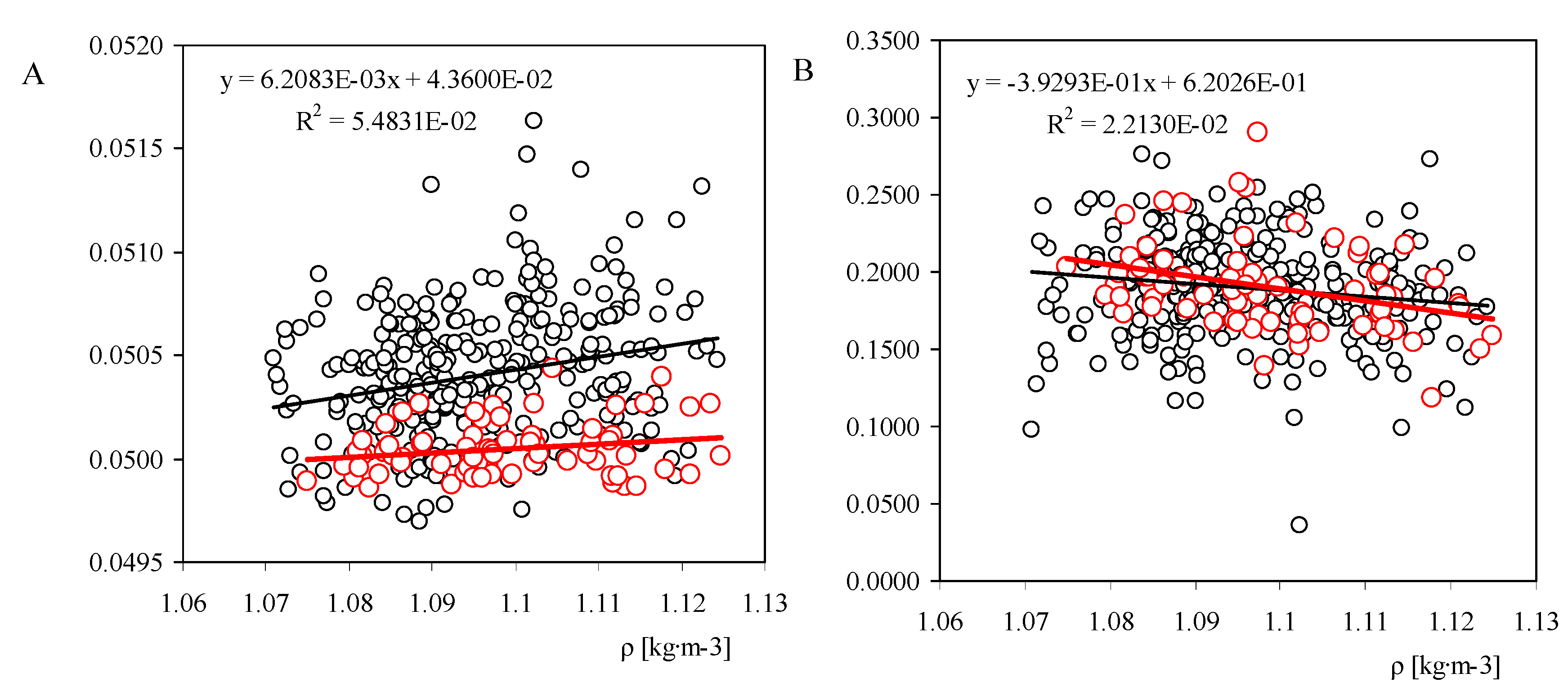
In
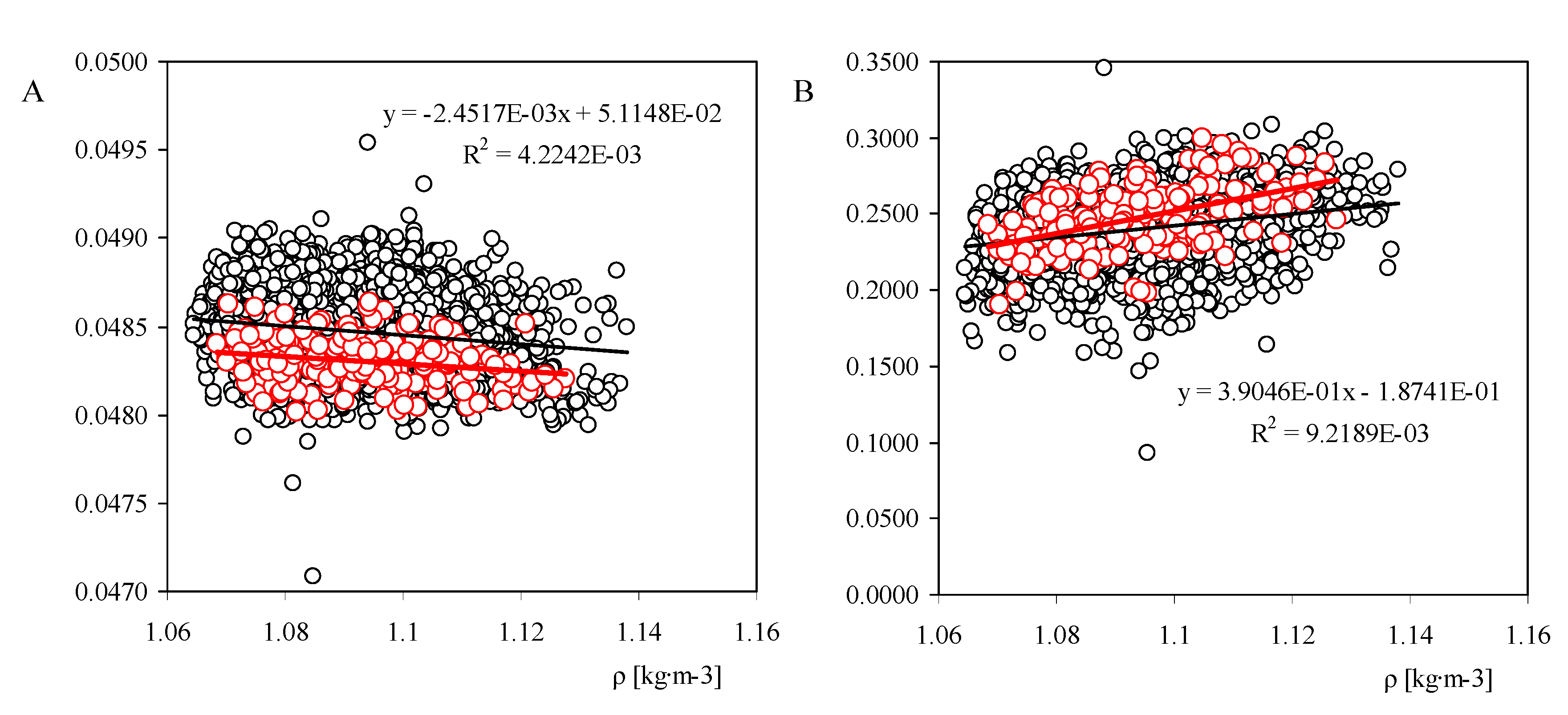
Figure 4 and
Figure 5, the values of constants A and B with regard to the calibrations performed on Thies Clima 4.3350 and Vector Instruments A100 L2 anemometer models, together with data related to the corresponding IDR/UPM Institute anemometer as a function of the air density are shown, respectively. In these two figures the general behavior of an anemometer model with changes in the air density can be compared to the behavior of a single individual anemometer. Despite the linearity shown in
Figure 4 and
Figure 5, some differences between the data corresponding to an anemometer model and the one with regard to a single individual anemometer can be observed, the slopes of the linear fittings being different.
Other obvious difference between the behavior of the single individual anemometer and the behavior of its corresponding general model remains on the standard deviation of the data. The standard deviation values of the data with regard to the considered density brackets, see
Table 3 and
Table 5, are lower in the case of the individual anemometers. Comparing the average values (calculated from all air density brackets) of the standard deviations the following values are obtained:
σA = 1.3989 × 10
−4 and
σB = 2.506 × 10
−2 (Vector Instruments A100 L2), and
σA = 1.3107 × 10
−4 and
σB = 1.7465 × 10
−2 (Thies Clima 4.3350) regarding to the individual anemometers, and
σA = 3.0761 × 10
−4 and
σB = 3.2293 × 10
−2 (Vector Instruments A100 L2), and
σA = 3.1142 × 10
−4 and
σB = 3.1046 × 10
−2 (Thies Clima 4.3350) with regard to the anemometers models.
Figure 4.
Calibration constants,
A and
B, measured for the Vector Instruments A100 L2 model anemometers, as a function of the air density value,
ρ, during the calibrations. The linear fit to the data has been included in the graphs. The data correspondent to the IDR/UPM Institute Vector Instruments A100 L2 anemometer calibration results as a function of the air density (see
Figure 2), has been also included in both graphs in red color.
Figure 5.
Calibration constants,
A and
B, measured for the Thies Clima 4.3350 model anemometers, as a function of the air density value,
ρ, during the calibrations. The linear fit to the data has been included in the graphs. The linear fit correspondent to the IDR/UPM Institute Thies Clima 4.3350 anemometer calibration results as a function of the air density (see
Figure 2), has been also included in both graphs (red color line).
As previously mentioned, these differences are quite obvious, as the standard deviations corresponding to the anemometers models take into account the variations due to the fabrication process. However, thanks to this comparison, it is possible to make a first estimation of the standard deviation values of a single individual anemometer, based on the data from the calibrations performed on multiple anemometers of the same model, that is, σA and σB, will have to be respectively reduced to 42% to 46% and from 56% to 78% of their value.
Based on the calibration constants A and B, variations as a function on the density, it is possible to estimate the measured wind speed deviation of an anemometer due to changes in air density, ∆
ρ. If a Gaussian process is considered, this deviation can be expressed as:
with around 46.5% confidence level. In the previous Equation,
V is the reference wind speed,
dA/
dρ and
dB/
dρare the slopes of the linear fittings to the data (see
Figure 3a–d and
Table 4), and
σA and
σB are standard deviations (an average value from
Table 5 can be selected, taken into account that there are no big variations of the standard deviations from one density bracket to another).
λA and
λB are the reduction coefficients with regard to the mentioned standard deviations, considering the behavior of a single individual anemometer from the data related to the calibrations performed on multiple anemometers of the same model (
λA = 0.46 and
λB = 0.78 were considered based on the aforementioned comparison between the single individual case and the general model’s behavior with regard to the Vector Instruments A100 L2 and Thies Clima 4.3350 anemometers). Finally, A
0 and B
0 are the calibration constants of the anemometer considered. These constants are introduced in the formula in order to study the wind speed variations as a function of the reference wind speed instead of the anemometers output frequency,
f.
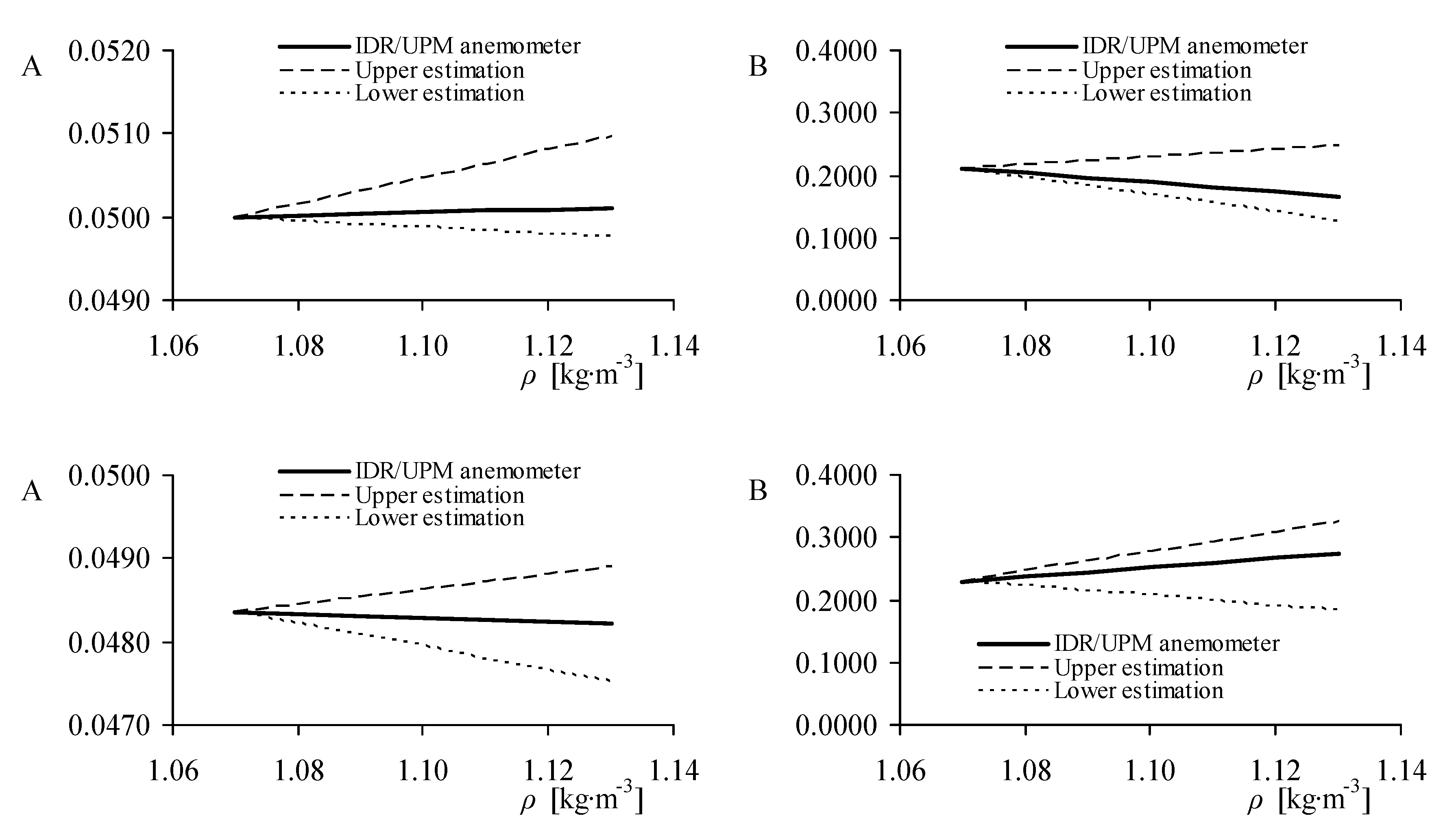
In order to check the proposed estimation for the wind speed variations with the air density, the upper and lower values of the calibration constants have been calculated for the Vector Instruments A100 L2 and Thies Clima 4.3350 IDR/UPM anemometers as a function of the air density, starting at
ρ = 1.07 kg·m
−3. The results are shown in
Figure 6. It can be observed that the behavior of the two single individual anemometers calibration constants has been correctly estimated between the upper and lower limits proposed.
The previous estimation procedure has been used to analyze the effect of air density changes on other anemometer models behavior. In
Table 6, the percentage variation intervals of the measured wind speed due to a change in the air density ∆
ρ = 0.1 kg·m
−3, estimated with Equation (5), have been included for the analyzed anemometer models together with the IDR/UPM Vector Instruments A100 L2 and Thies Clima 4.3350 anemometers. Obviously, in these two cases the correction coefficients were
λA = 0 and
λB = 0. The correction coefficients used in the general (not specific) cases were the same as the ones introduced for the A100 L2 and Thies Clima 4.3350 anemometers, that is,
λA = 0.46 and
λB = 0.78. As these coefficients were very similar for the aforementioned anemometers, it seems reasonable to suppose that there will be no big differences with the ones related to other anemometer models. The calibration constants, A
0 and B
0, in all cases where calculated (see
Table 2 and
Table 4) for
ρ = 1.09 kg·m
−3 air density, as this value corresponds to the average ambient conditions at the IDR/UPM Institute. It can be observed in
Table 6 that the estimated variations of measured wind speed for the two single individual anemometers are not exactly the ones estimated for the corresponding anemometer’s model, however, they are of the same order (specially the one with regard to the Thies Clima 4.3350 anemometer). From these results it seems that the variations of measured wind speed due to a change in the air density ∆
ρ = 0.1 kg·m
−3, could be relevant. In
Table 7a and b, the Annual Energy Production (AEP) of a 2.5 MW wind turbine (GE2.5, see Reference [
3] for more information) has been estimated for 4, 7, and 10 m s
−1 annual average wind speed. It should also be said that taking into account that the air density variation with regard to the data in
Figure 2 and
Figure 3 is ∆
ρ ~ 0.05 kg·m
−3, the AEP estimations for ∆
ρ = 0.1 kg·m
−3 can be considered a rough extrapolation. However, it indicates the quite large deviation of AEP estimations, if changes in the air density are not considered.
Figure 6.
Variation of the IDR/UPM anemometers (
Top: Vector Instruments A100 L2; and
bottom: Thies Clima 4.3350) calibration constants
A and
B with air density, starting from
ρ = 1.07 kg·m
−3. In the graphs, the linear fittings from the data (
Table 2 and
Figure 2), are compared to the upper and lower estimations.
Table 6.
Percentage variation interval (around 46.5% confidence, assuming a Gaussian process), of the measured wind speed due to a density variation of ∆ρ = 0.1 kg·m−3, for the analyzed anemometer models and the two IDR/UPM anemometers.
Table 6.
Percentage variation interval (around 46.5% confidence, assuming a Gaussian process), of the measured wind speed due to a density variation of ∆ρ = 0.1 kg·m−3, for the analyzed anemometer models and the two IDR/UPM anemometers.
| Anemometer | V = 4 m s−1 | V = 7 m s−1 | V = 10 m s−1 |
|---|
| lower limit | upper limit | lower limit | upper limit | lower limit | upper limit |
|---|
| NRG Systems Maximum 40/40C | −2.71% | 3.58% | −1.83% | 2.35% | −1.47% | 1.86% |
| Secondwind C3 | −2.79% | 1.77% | −2.03% | 1.11% | −1.73% | 0.84% |
| TH 4.3350 | −1.48% | 2.48% | −1.34% | 1.48% | −1.29% | 1.08% |
| TH 4.3351 | 0.01% | 1.72% | −0.13% | 1.00% | −0.19% | 0.72% |
| TH 4.3303 | −9.21% | 1.57% | −5.36% | 1.79% | −3.83% | 1.88% |
| A100 L2 | −1.50% | 1.89% | −0.57% | 1.84% | −0.19% | 1.82% |
| A100 LK | −1.71% | 2.16% | −1.18% | 1.58% | −0.97% | 1.34% |
| Ornytion 107A | −1.09% | 1.27% | −0.91% | 0.77% | −0.83% | 0.58% |
| RM Young 3002/3102 | −21.14% | 6.24% | −12.33% | 4.41% | −8.80% | 3.68% |
| RM Young 05103 | −1.42% | 3.31% | −0.93% | 2.24% | −0.74% | 1.81% |
| A100 L2 (IDR/UPM) | −3.48% | 0.56% | −2.05% | 0.75% | −1.47% | 0.82% |
| TH 4.3350 (IDR/UPM) | 0.02% | 2.35% | −0.40% | 1.26% | −0.57% | 0.82% |
Table 7.
Deviation of the AEP due to variations in wind speed measurements caused by variations of the air density, ∆ρ = 0.05 kg·m−3, and ∆ρ = 0.1 kg·m−3, as a function of the annual average wind speed (4 m·s−1, 7 m·s−1 and 10 m·s−1), and the anemometer considered.
(a)
| NRG Systems Maximum 40/40C |
| Annual average wind speed | ∆ρ = 0.05 kg·m−3 | ∆ρ = 0.1 kg·m−3 |
| Lower limit | Upper limit | Lower limit | Upper limit |
| 4 m·s−1 | −10.08% | 13.19% | −20.15% | 26.37% |
| 7 m·s−1 | −5.17% | 5.76% | −10.34% | 11.53% |
| 10 m·s−1 | −2.93% | 3.09% | −5.86% | 6.17% |
| Secondwind C3 |
| Annual average wind speed | ∆ρ = 0.05 kg·m−3 | ∆ρ = 0.1 kg·m−3 |
| Lower limit | Upper limit | Lower limit | Upper limit |
| 4 m·s−1 | −8.83% | 8.89% | −17.66% | 17.78% |
| 7 m·s−1 | −4.63% | 3.94% | −9.27% | 7.88% |
| 10 m·s−1 | −2.64% | 2.12% | −5.28% | 4.23% |
| Thies Clima 4.3350 |
| Annual average wind speed | ∆ρ = 0.05 kg·m−3 | ∆ρ = 0.1 kg·m−3 |
| Lower limit | Upper limit | Lower limit | Upper limit |
| 4 m·s−1 | −7.30% | 9.28% | −14.60% | 18.56% |
| 7 m·s−1 | −3.98% | 4.10% | −7.96% | 8.19% |
| 10 m·s−1 | −2.29% | 2.20% | −4.58% | 4.40% |
| Thies Clima 4.3351 |
| Annual average wind speed | ∆ρ = 0.05 kg·m−3 | ∆ρ = 0.1 kg·m−3 |
| Lower limit | Upper limit | Lower limit | Upper limit |
| 4 m·s−1 | −2.11% | 4.41% | −4.22% | 8.82% |
| 7 m·s−1 | −1.15% | 1.86% | −2.30% | 3.73% |
| 10 m·s−1 | −0.66% | 0.99% | −1.32% | 1.98% |
| Thies Clima 4.3303 |
| Annual average wind speed | ∆ρ = 0.05 kg·m−3 | ∆ρ = 0.1 kg·m−3 |
| Lower limit | Upper limit | Lower limit | Upper limit |
| 4 m·s−1 | −21.12% | 17.49% | −42.23% | 34.97% |
| 7 m·s−1 | −10.45% | 8.03% | −20.89% | 16.06% |
| 10 m·s−1 | −5.87% | 4.36% | −11.73% | 8.71% |
| Vector Instruments A100 L2 |
| Annual average wind speed | ∆ρ = 0.05 kg·m−3 | ∆ρ = 0.1 kg·m−3 |
| Lower limit | Upper limit | Lower limit | Upper limit |
| 4 m·s−1 | −5.56% | 8.59% | −11.12% | 17.17% |
| 7 m·s−1 | −2.77% | 4.08% | −5.53% | 8.15% |
| 10 m·s−1 | −1.55% | 2.23% | −3.11% | 4.46% |
(b)
| Vector Instruments A100 LK |
| Annual average wind speed | ∆ρ = 0.05 kg·m−3 | ∆ρ = 0.1 kg·m−3 |
| Lower limit | Upper limit | Lower limit | Upper limit |
| 4 m·s−1 | −7.07% | 9.15% | −14.13% | 18.31% |
| 7 m·s−1 | −3.74% | 4.17% | −7.47% | 8.33% |
| 10 m·s−1 | −2.14% | 2.26% | −4.27% | 4.51% |
| Ornytion 107A |
| Annual average wind speed | ∆ρ = 0.05 kg·m−3 | ∆ρ = 0.1 kg·m−3 |
| Lower limit | Upper limit | Lower limit | Upper limit |
| 4 m·s−1 | −4.55% | 5.31% | −9.09% | 10.61% |
| 7 m·s−1 | −2.46% | 2.36% | −4.92% | 4.72% |
| 10 m·s−1 | −1.41% | 1.27% | −2.83% | 2.54% |
| RM Young 3002/3102 |
| Annual average wind speed | ∆ρ = 0.05 kg·m−3 | ∆ρ = 0.1 kg·m−3 |
| Lower limit | Upper limit | Lower limit | Upper limit |
| 4 m·s−1 | −45.92% | 38.94% | −91.83% | 77.87% |
| 7 m·s−1 | −21.92% | 16.51% | −43.84% | 33.03% |
| 10 m·s−1 | −12.18% | 8.78% | −24.37% | 17.55% |
| RM Young 05103 |
| Annual average wind speed | ∆ρ = 0.05 kg·m−3 | ∆ρ = 0.1 kg·m−3 |
| Lower limit | Upper limit | Lower limit | Upper limit |
| 4 m·s−1 | −7.03% | 10.99% | −14.05% | 21.98% |
| 7 m·s−1 | −3.62% | 4.83% | −7.24% | 9.66% |
| 10 m·s−1 | −2.05% | 2.59% | −4.11% | 5.19% |


