Article

Entropy-Based Bagging for Fault Prediction of Transformers Using Oil-Dissolved Gas Data

State Key Laboratory of Power Transmission Equipment & System Security and New Technology, Chongqing University, 174 Shazheng Street, Chongqing 400044, China
*
Author to whom correspondence should be addressed.
Energies 2011, 4(8), 1138-1147; https://doi.org/10.3390/en4081138
Submission received: 28 February 2011 / Revised: 21 July 2011 / Accepted: 1 August 2011 / Published: 4 August 2011
(This article belongs to the Special Issue Future Grid)

Abstract

:
The development of the smart grid has resulted in new requirements for fault prediction of power transformers. This paper presents an entropy-based Bagging (E-Bagging) method for prediction of characteristic parameters related to power transformers faults. A parameter of comprehensive information entropy of sample data is brought forward to improve the resampling process of the E-Bagging method. The generalization ability of the E-Bagging is enhanced significantly by the comprehensive information entropy. A total of sets of 1200 oil-dissolved gas data of transformers are used as examples of fault prediction. The comparisons between the E-Bagging and the traditional Bagging and individual prediction approaches are presented. The results show that the E-Bagging possesses higher accuracy and greater stability of prediction than the traditional Bagging and individual prediction approaches.

1. Introduction

Prediction of potential failures in electrical power equipment can effectively improve the reliability of electrical grids. Because power transformers are very important electrical power equipment in electrical grids, their failure prediction has been focused on by a lot of researchers. Prediction of failures in power transformers consists of two steps. The first is to estimate characteristic parameters of transformer faults based on sample data related to transformer conditions. Secondly, a fault diagnostic tool is used to evaluate transformer faults in combination with the estimated characteristic parameters. Many approaches, including regression analysis [1], time series analysis [2], artificial neural networks (ANN) [3,4,5], grey models (GM) [6,7], and support vector machines (SVM) [8], have been used to estimate the characteristic parameters of transformer faults. Estimation accuracy of these approaches can be acceptable if sample data with sufficient accuracy is available. However, sample data of transformer faults may be obtained from various sources and the accuracy levels of the sample data may be different. Based on sample data of transformer faults with different accuracy levels, a fault prediction model may generate different characteristic transformer fault parameters results. How to design a robust model of transformer fault prediction and improve generalization ability of the prediction model is still a task that is attracting more and more researchers.
Ensemble learning is an effective approach to enhance generalization of machine learning algorithms. Bagging [9] and Adaboost [10] are two major ensemble learning methods to form a combined classifier or predictive tool based on data resampling. They are capable of improving stability of classification or prediction models as well as keeping maximum time complexity of the models unchanged. Adaboost is adapted to combine weak classification or prediction models with strong independence, while Bagging is applicable to combine strong classification or prediction models. Some approaches, such as sub-Bagging [11] and weighted member models [12], were brought forward to improve ensemble learning with satisfactory results.
This paper presents an improved Bagging algorithm for power transformer fault prediction based on oil-dissolved gas. The improved bagging is also called entropy-based Bagging (E-Bagging), because comprehensive information entropy was considered to improve Bagging. The probability of selecting sample data for training is determined by the comprehensive information entropy of the sample data. Sample data containing a greater amount of information results in bigger comprehensive entropy of the sample data and has a greater probability of being selected for training. Examples and analysis results show that the improved Bagging enhances generalization and accuracy of transformer fault prediction based on oil-dissolved gas.

2. Algorithm of Entropy-Based Bagging

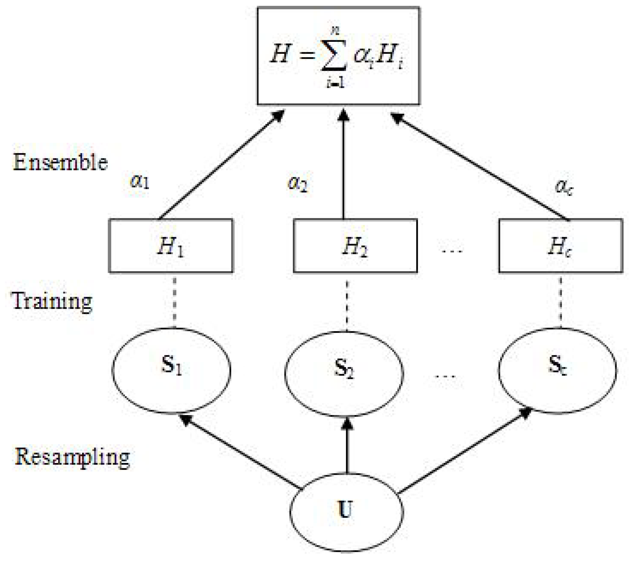
2.1. Basic Process of Bagging

As shown in Figure 1, Bagging is a parallel process to train a machine learning algorithm. Data subsets from S1 to Sn are randomly selected from the whole data set U for training. This process is called a sample data resampling process. The data subset Si is used for training to obtain a member prediction function Hi. Many popular methods, such as SVM [8], ANN [3,4,5], and GM [6,7], could be used to construct the member prediction function. The combined prediction function H is deducted from the member functions H1, H2, ⋯, Hc by a weighted mean method as below [13]:
H = i = 1 c α i H i
where αi is the weight of member prediction function Hi and αi = 1/c.
In Figure 1, Hi could be a very time-wasting prediction model, like an artificial neural network. If the whole sample data are used for training the individual prediction model, time for training may be too much to be acceptable. However, each data subset has a much smaller size than the whole sample data, so the time to train an individual model by using a data subset can be reduced considerably. The Bagging method can thus save much time in training all individual models in the parallel process and thus form the combined prediction model.
Figure 1. Basic process of Bagging for an ensemble of prediction functions.
Energies 04 01138 g001
The parallel process of Bagging shows that resampling is a very important step to select representative sample data for training. It may influence the diagnosis or prediction results of Bagging. The usual process of resampling is a simple random selection of sample data without prior information. This indicates that the probability of sample data being selected is same. The simple random resampling may not improve or even reduce the accuracy of diagnosis or prediction results of Bagging.

2.2. Data Resampling Based on Comprehensive Information Entropy

Sample data of transformer faults come from transformers at different voltage levels and under various operation conditions. The representative sample data should be selected with great probability during the resampling process of Bagging. A uniform standard is thus required to determine the probability of sample data for selection. A comprehensive information entropy parameter of sample data is introduced as below to determine selection probability of the data. The comprehensive information entropy is a weighted sample entropy of the sample data.

2.2.1. Computation of Sample Entropy

Information entropy is a measure of the uncertainty associated with a random variable in information theory. Sample entropy was proposed as a complexity measure of time series in [14]. In this paper, it is used as an objective measure of the amount of information contained in sample data.
Let U = [u1, u2, ⋯, un] denote a n-elements sample data sequence of transformer faults. The computation algorithm of sample entropy of the data sequence consists of the following steps:
(1)
Form a set of m sample data segment defined as:
X ( i ) = [ u i , u i + 1 , ... , u i + m 1 ] ,        i [ 1 , N m + 1 ]
(2)
Calculate d[X(i), X(j)], the distance between X(i) and X(j), defined as the maximum absolute difference between any two vectors of the two sample data segments:
d [ X ( i ) , X ( j ) ] = max [ | u i + k u j + k | ] ,      k [ 0 , m 1 ] ;   i , j [ 1 , N m + 1 ]
If ui is a q-dimensional vector, the value of | u i + k u j + k | is calculated as below:
| u i + k u j + k | = t = 1 q [ u i + k ( t ) u j + k ( t ) ] 2
(3)
Given a tolerance parameter r, calculate the number whereby d [ X ( i ) , X ( j ) ] is smaller than r. B i m ( r ) is a measure to describe the similarity degree between the sample data segment X(i) and the sample data sequence U. B i m ( r ) is defined as:
B i m ( r ) = 1 N m { count ( d [ X ( i ) , X ( j ) ] < r ) } ,      j [ 1 , N m + 1 ] ,   i j
where the function count(·) is to calculate the number that d [ X ( i ) , X ( j ) ] is smaller than r.
(4)
For i∈[1, Nm + 1], calculate the average of B i m ( r ) as below:
B m ( r ) = 1 N m + 1 i = 1 N m + 1 B i m ( r ) ,     i [ 1 , N m + 1 ]
(5)
Form a new set of m+1 sample data sequence as below:
Z ( i ) = [ u i , u i + 1 , ... , u i + m ] ,        i [ 1 , N m ]
For i∈[1, Nm + 1], calculate A i m ( r ) and A m ( r ) as follows:
A i m ( r ) = 1 N m 1 { count ( d [ Z ( i ) , Z ( j ) ] < r ) } ,      j [ 1 , N m ] ,   i j
A m ( r ) = 1 N m i = 1 N m A i m ( r ) ,     i [ 1 , N m ]
(6)
Calculate the sample entropy E of the sample data sequence as:
E ( m , r ) = lim N { ln [ A m ( r ) / B m ( r ) ] }
When N is a finite number, the sample entropy of the sample data sequence can be estimated as:
E ( m , r ) = ln [ A m ( r ) / B m ( r ) ]

2.2.2. Comprehensive Information Entropy

Comprehensive information entropy of the sample data segment ui is defined as:
ξ(ui) = ωiEi(m,r)
where ωi is an additional weight of the sample entropy.
Suppose Y = [y1, y2, ⋯, yn] to be a data sequence about additional information of transformers. Given a target vector y ^ , the additional weight of sample entropy can be computed as:
ω i = 1 1 n k = 1 n y i k y ^ k Max [ | y k ¯ y ^ k | , | y k ¯ y ^ k | ]
where yik is the kth element of the vector yi and y ^ k is the kth element of the target vector y ^ . y k ¯ and y k ¯ represent maximum and minimum of the kth elements of all vectors belonging to Y, respectively. The additional weight of sample entropy is a normalized parameter between 0 and 1.

2.2.3. Procedures of Data Resampling

Probability of data to be selected for training is calculated as:
p ( u i ) = ξ ( u i ) / j = 1 n ξ ( u j )
Given a vector I1 with m elements equal to zero and m < n, where n is the number of sample data and the selected sample data is noted as S1. The procedures of data resampling algorithm are as follows:
(1)
Generate randomly a vector R = [r1,r2, ⋯ ,rn], where ri is a random number between 0 and 1;
(2)
Let k = 0 and form a vector T = [r1p(u1),r1p(u2), ⋯ ,rnp(un)];
(3)
Find the index corresponding to the maximum element of T;
(4)
Let k = k + 1, T(k) = 0, and give the index to I1(k);
(5)
Let S1(k) = U[I1(k)];
(6)
Repeat steps from (3) to (5) until k = m.
If the Bagging consists of member prediction functions in number of c, the above procedures are repeated to obtain S1, S2, ⋯, Sc for training.

2.2.4. E-Bagging Procedures

The procedures of the E-Bagging algorithm are as follows:
(1)
Calculate the comprehensive information entropy of sample data by using (12) to obtain Si, where I = 1, 2, ⋯, c;
(2)
Use Si to train the member prediction function Hi;
(3)
Repeat steps (1) and (2) until the completion of training of the member prediction function Hc;
(4)
Combine the member prediction functions H1, H2, ⋯, Hc to obtain the ensemble prediction function H by using (1).
From the above E-Bagging procedures, it could be found that the traditional Bagging is a special case of the E-Bagging when ξ ( u i ) 1 . The maximum time complexity to compute the comprehensive information entropy of the E-Bagging algorithm is O (mNc), where m is the number of sample data of every subset, N is the number of the whole sample data, and c is the number of data subsets. This is much shorter than the time required for a member prediction algorithm used in the E-Bagging. Therefore, the time complexity of the E-Bagging algorithm is the same as that of the traditional Bagging algorithm.

3. Examples of Transformer Fault Prediction

3.1. Processing of Sample Data

The fault prediction of transformers is based on a total of 1200 sample datasets of oil-dissolved gas in oils of transformers with voltage levels between 50 kV and 220 kV. The sample data are normalized as:
u ^ i j = u i j / j = 1 5 u i j
where uij is the jth element of the sample data ui. Because the elements of each sample data vector correspond to the measurement results of the five types of oil-dissolved gas: H2, CH4, C2H2, C2H4, and C2H6, the sample data ui = [ui1, ui2, ui3, ui4, ui5].
Voltage level and operation time of transformers are two additional information items of transformers. Table 1 shows the voltage levels and participation of operation time of transformers. The mapping values of the additional information of transformers are also presented in Table 1. Every data vector about additional information of transformers thus consists of two elements according to Table 1. For example, if yi denotes a sample data about additional information of a 110 kV and 15 years transformers, yi = [2, 3].
Table 1. Mapping values of additional information of transformers.
Additional InformationTypesMapping Values
Voltage levels (kV)351
1102
2203
Running time (Year)[0, 5)1
(5, 10]2
(10, 15]3
(15, 20]4
(20, ∞)5

3.2. Results and Analysis

3.2.1. Prediction Accuracy

Table 2 shows the average relative errors of prediction results of the E-Bagging. Four prediction models, GM [6], SVM [8], back-propagation neural network (BPNN) [5], and a combination forecasting method (CF) [15] based on the previous three prediction models, are used as individual models for Bagging. For the E-Bagging, the size of each data subset m = 400 and number of member functions c = 10. The average relative errors of these four models and traditional Bagging based on the four models are also presented in Table 2.
Table 2. Average relative error of fault prediction.
ModelE-BaggingBaggingIndividual
CF3.01%3.48%4.80%
SVM6.03%6.53%7.41%
BPNN6.12%6.44%7.53%
GM6.94%7.01%7.91%
As can be seen from Table 2, the average relative errors of the E-Bagging are smaller than those of both the Bagging and the individual models. This indicates that the improvements of the E-Bagging are capable of increasing the transformer fault prediction accuracy.

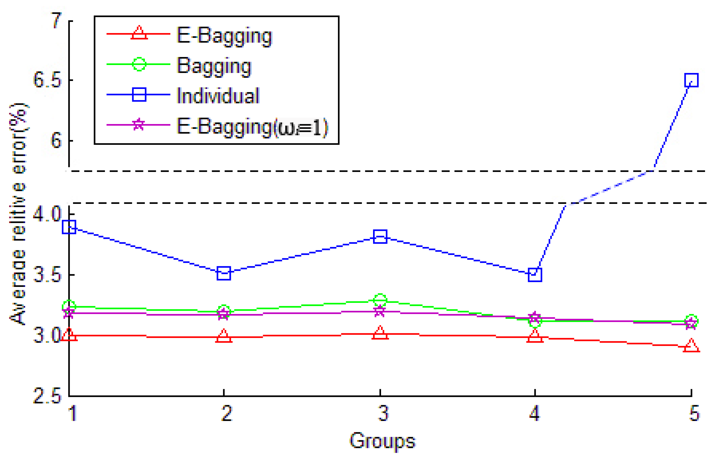
3.2.2. Prediction Stability

The above 1200 sample datasets were divided into five groups for testing the prediction stability of E-Bagging. The first group consists of 800 sample data. The first 100 sample data of the first group were replaced by the first 100 of the remaining 400 sample data to obtain the second group of sample data. The third group was obtained by taking the first 200 from the remaining 400 sample data to replace the first 200 sample data of the first group. By the same way, 100 more sample data of the first group were replaced each time to obtain the other two groups of sample data. From the first group to the fifth group, changes of sample data increases. The five groups of sample data were used as for training, respectively.
Table 3 shows the average relative errors of the E-Bagging, Bagging, and individual models, which are trained by using the five groups of sample data. The prediction of E-Bagging is stable, even though various sample data are used for its training. However, the average relative errors of individual models change more than the E-Bagging when the five groups of sample data are used for training.
Table 3. Average relative error of fault prediction.
Group No.Individual ModelE-BaggingE-Bagging (ωi≡ 1)BaggingIndividual
Group 1CF2.99%3.18%3.23%3.90%
SVM6.23%6.59%6.69%7.81%
BPNN6.28%6.43%6.68%7.83%
GM6.94%7.01%7.21%8.01%
Group 2CF2.98%3.17%3.20%3.51%
SVM6.21%6.41%6.61%7.21%
BPNN6.29%6.50%6.72%8.43%
GM6.92%7.07%7.29%8.69%
Group 3CF3.01%3.20%3.29%3.82%
SVM6.20%6.45%6.56%7.95%
BPNN6.29%6.46%6.71%7.01%
GM6.97%6.95%7.33%8.92%
Group 4CF2.98%3.14%3.11%3.50%
SVM6.22%6.39%6.53%7.21%
BPNN6.24%6.29%6.43%8.83%
GM7.02%6.94%7.10%8.57%
Group 5CF2.91%3.09%3.12%6.51%
SVM6.01%6.49%6.51%9.51%
BPNN6.12%6.35%6.42%8.99%
GM6.88%6.96%8.16%10.28%
Figure 2 shows furthermore the average relative errors of the E-Bagging, Bagging, and CF. The CF is the individual model of both the E-Bagging and the Bagging. The change of the average relative error of E-Bagging based on CF is smallest among the three prediction approaches. The CF generates the much greater change of the average relative error of prediction than the E-Bagging and Bagging, if no ensemble is used.
Figure 2. Error rate of CF by different ensemble methods.
Energies 04 01138 g002
To compare the stability of the prediction methods, the standard deviation σ of average relative error is used as quantification measure as below:
σ = 1 n i = 1 n ( e i e ¯ ) 2
where ei is the average relative error of fault prediction and e is the average of ei.
Table 4 shows the calculation results of the standard deviation of average relative errors of prediction by using the E-Bagging, Bagging, and the individual models. Except for the SVM used for ensemble, the E-Bagging generates a significantly smaller standard deviation of the average relative error of fault prediction. The E-Bagging also generates much smaller standard deviation of the average relative error of fault prediction than the individual models. Table 4 also shows that the standard deviation of average relative error of E-Bagging when ωi ≡ 1. The additional weight of sample entropy can be used to increase the stability of E-Bagging, except for the SVM used for the ensemble.
Table 4. Standard deviation of average relative error of fault prediction.
E-BaggingE-Bagging (ωi ≡ 1)BaggingIndividual
CF0.0003380.0003830.0006780.011424
SVM0.0008260.0007090.0006450.008423
BPNN0.0006470.0007610.0013700.007246
GM0.0004720.0004840.0037920.007550

4. Conclusions

This paper presents an E-Bagging method based on the comprehensive information entropy. The examples and analysis of transformer fault prediction are also presented. The results of the work can be summarized as follows:
(1)
The resampling is an important process of Bagging. The comprehensive information entropy of sample data is helpful to select representative sample data for training during the resampling process and to improve the generalization ability of Bagging.
(2)
The E-Bagging method improves the prediction accuracy of transformer faults. E-Bagging generates significantly smaller average relative transformer fault prediction errors, based on 1200 sample data of oil-dissolved gas, than the traditional Bagging and individual prediction algorithms.
(3)
E-Bagging shows a good generalization ability of prediction of transformer faults. The stability of the E-Bagging was shown to be greater than the traditional Bagging and individual prediction algorithms through examples of training with various sample data.

Acknowledgements

The authors acknowledge the fund of 863 Program of China (2009AA04Z416) to support this work. The National Science Foundation of China (51021005) and the Natural Science Foundation of Chongqing, China (CSTC 2009BA4048) are also appreciated for supporting this work.

References

  1. Wu, C.J.; Hu, C.H.; Yen, S.S.; Yin, C.C.; Chiu, C.C.; Lee, Y.M. Application of regression models to predict harmonic voltage and current growth trend from measurement data at secondary substations. IEEE Trans. Power Deliv. 1998, 13, 793–799. [Google Scholar]
  2. Zhou, L.J.; Wu, G.N.; Zhang, X.H.; Zhu, K. prediction of power transformer faults based on time series of weighted fuzzy degree analysis. Autom. Electr. Power Syst. 2005, 29, 53–55. [Google Scholar] [CrossRef]
  3. Wahab, M.A.A.; Hamada, M.M.; Mohamed, A. Artificial neural network and non-linear models for prediction of transformer oil residual operating time. Electr. Power Syst. Res. 2011, 1, 219–227. [Google Scholar] [CrossRef]
  4. Shaban, K.; El-Hag, A.; Matveev, A. A cascade of artificial neural networks to predict transformers oil parameters. IEEE Trans. Dielectr. Electr. Insul. 2009, 16, 516–523. [Google Scholar] [CrossRef]
  5. Sencan, A.; Kizilkan, O.; Bezir, N.C.; Kalogirou, S.A. Different methods for modeling absorption heat transformer powered by solar pond. Energy Convers. Manag. 2007, 3, 724–735. [Google Scholar] [CrossRef]
  6. Wang, Y.Y.; Liao, R.J.; Sun, C.X.; Du, L.; Hu, J.L. A GA-based Grey Prediction Model for Predicting the Gas-in-oil Concentrations in Oil-filled Transformer. In Proceedings of the Conference Record of the 2004 IEEE International Symposium on Electrical Insulation, Indianapolis, IN, USA, September 2004; pp. 74–77.
  7. Song, B.; Peng, Z.H. Short-term forecast of the gas dissolved in power transformer using the hybrid grey model. Kybernetes 2009, 38, 489–496. [Google Scholar] [CrossRef]
  8. Yan, Z.; Zhang, B.D.; Yuan, Y.C.; Pei, Z.C. Transformer Fault Prediction Based on Support Vector Machine. In Proceedings of the 2nd International Conference on Computer Engineering and Technology, Chengdu, China, April 2010; pp. 513–516.
  9. Breiman, L. Bagging predictors. Mach. Learn. 1996, 8, 123–140. [Google Scholar]
  10. Ratsch, G.; Onoda, T.; Muller, K.R. Soft margins for adaboost. Mach. Learn. 2001, 3, 287–320. [Google Scholar] [CrossRef]
  11. Galvao, R.K.H.; Araujo, M.C.U.; Martins, M.D.; Jose, G.E.; Pontes, M.J.C.; Silva, E.C.; Saldanha, T.C.B. An application of subagging for the improvement of prediction accuracy of multivariate calibration models. Chemom. Intell. Lab. Syst. 2006, 3, 60–67. [Google Scholar] [CrossRef]
  12. Borra, S.; di Ciaccio, A. Improving nonparametric regression methods by bagging and boosting. Comput. Stat. Data Anal. 2002, 38, 407–420. [Google Scholar] [CrossRef]
  13. Oliveira, A.L.I.; Braga, P.L.; Lima, R.M.F.; Cornelio, M.L. GA-based method for feature selection and parameters optimization for machine learning regression applied to software effort estimation. Inf. Softw. Technol. 2010, 52, 1155–1166. [Google Scholar] [CrossRef]
  14. Richman, J.S.; Moorman, J.R. Physiological time-series analysis using approximate entropy and sample entropy. Am. J. Physiol. Heart Circ. Physiol. 2000, 278, H2039–H2049. [Google Scholar] [PubMed]
  15. Yang, T.F.; Liu, P.; Li, Z.; Zeng, X.J. A new combination forecasting model for concentration prediction of dissolved gases in transformer oil. Proc. CSEE 2008, 28, 108–113. [Google Scholar]

