Multiple Objective Compromised Method for Power Management in Virtual Power Plants


Abstract
:1. Introduction
2. Power Management in VPP
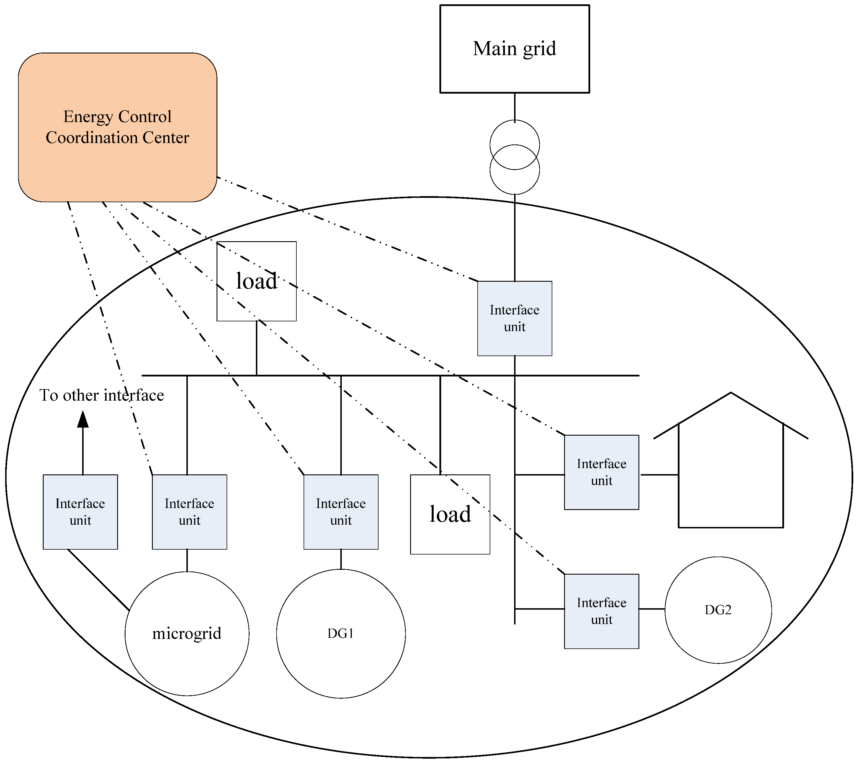
2.1. VPP as a Bridge between DERs and Public Grid

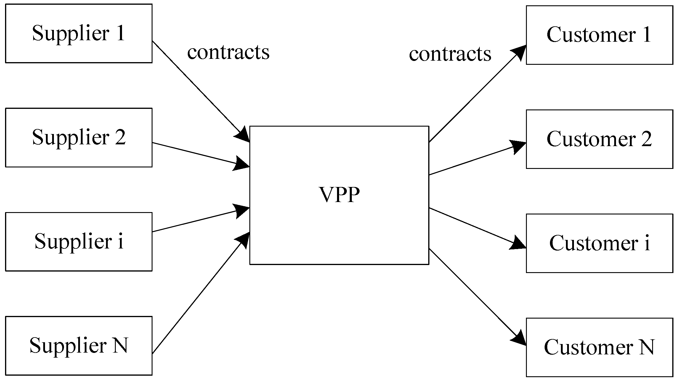
2.2. Electric Power Supply Chain in VPP
- (1)
- Microgrids, which have their own objectives and publish their output schedules in contracts;
- (2)
- Other suppliers which are scheduled by the VPP, such as wind farm or wind turbines which do not need any fuel, fuel batteries, and combined heat and power plants (CHP).
- (1)
- The sensitive loads which require high reliability and power quality with priority according to the contracts. Usually these loads are also predictable, such as industrial loads.
- (2)
- The public grid with the purchasing and selling contract. Form the view of the operators in public grid, it is expected the output power of the VPP is fixed to some extent according to the contrast especially when the power capacity of VPP is large.
- (3)
- The controllable load according to the load demand side management by ECCC [21].
- (4)
- The load which is random and can be shutdown in some situations according to the contracts, such as the smart houses and some unimportant loads.
- (1)
- The quantity and price of the electric power at different time segments;
- (2)
- Some special requirements for power reliability and power quality;
- (3)
- The fluctuating range of the set value;
- (4)
- The penalty methods.
3. Algorithm Formulation
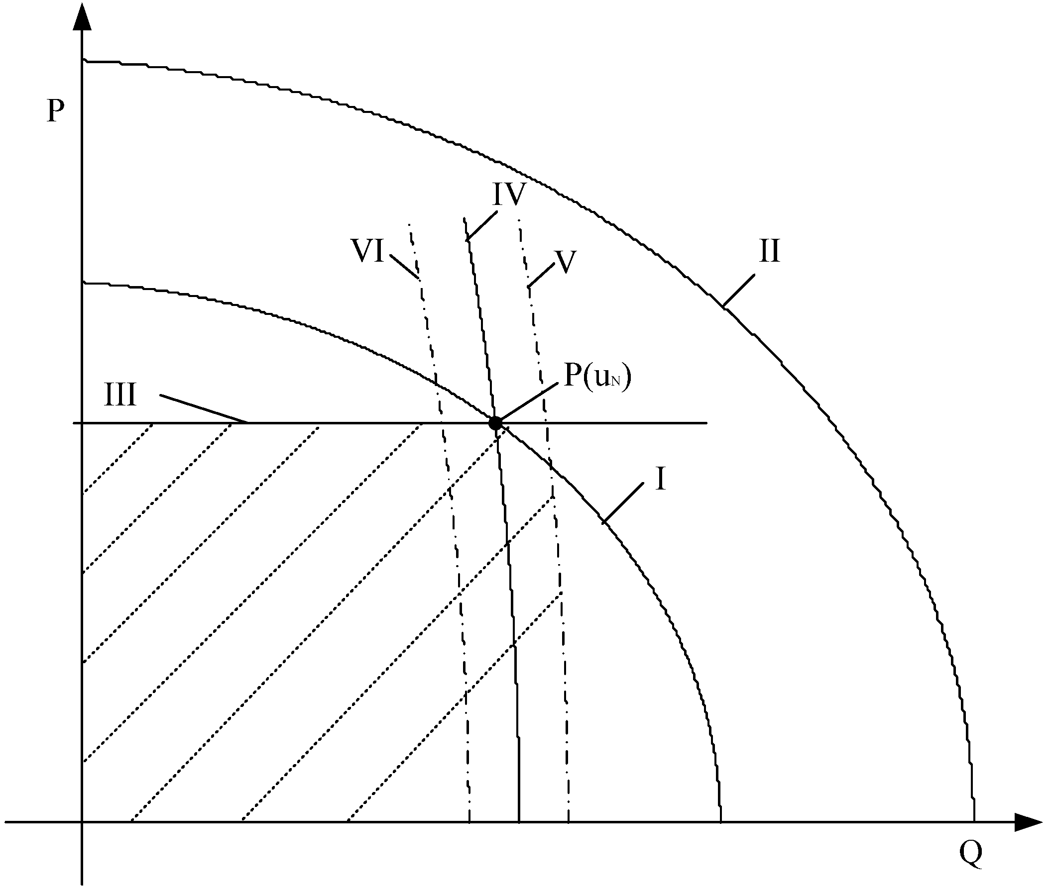
3.1. Multi-objective Optimization with Priority
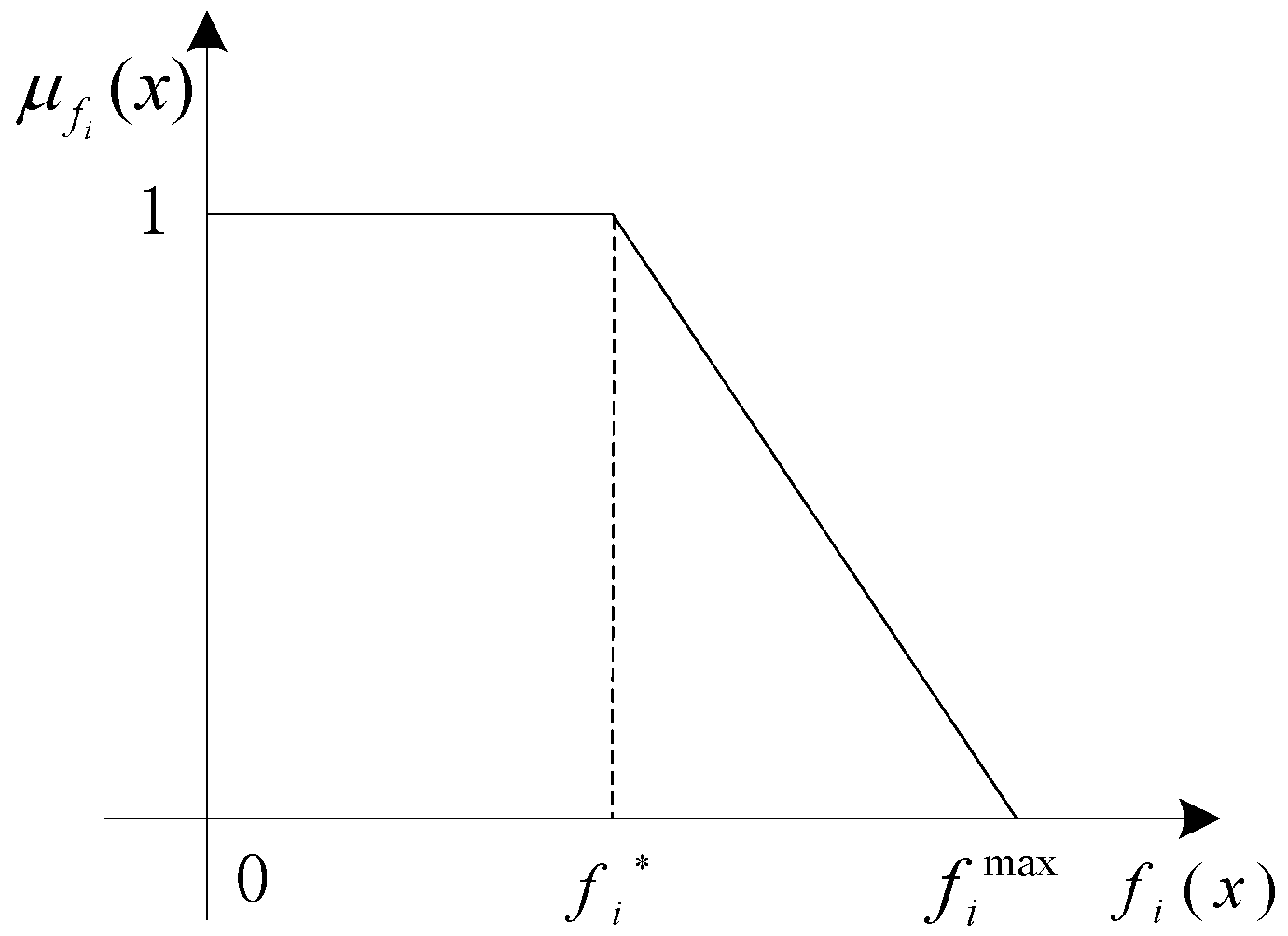
3.2. Fuzzy Description
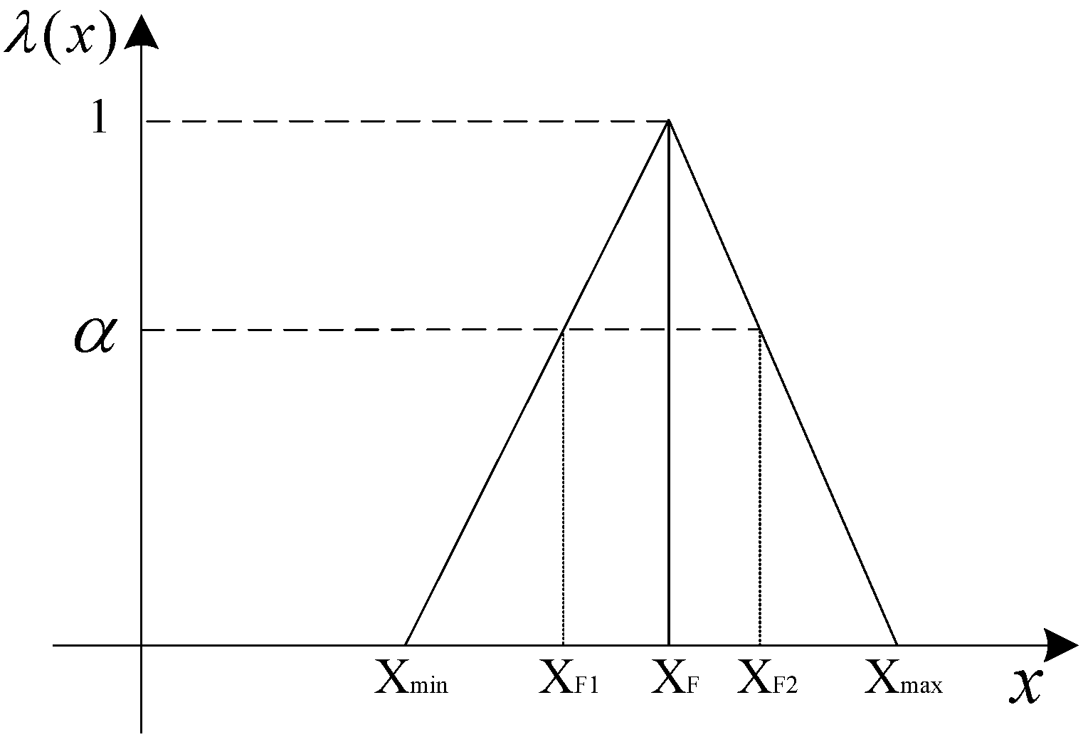
3.3. Two-Step Compromised Method
3.4. Objective Functions
- (1)
- the wind turbine and solar energy are preferred for environmental protection;
- (2)
- the output power to the public grid is preset one-day ahead;
- (3)
- the actual lines are represented as an ideal line with impedance;
- (4)
- the reliability requirements of the customers are satisfied by the suitable topology design of the VPP.
3.5. The Constraints of the Power Suppliers
- (1)
- All Feeder lines must operate within their line capacity. The transmission capability of the feed is a basic requirement in VPP operations.
- (2)
- The DGs should operate within the pre-specified maximum limit. The rated powers of the converters have to be pre-determined depending on the maximum power flowing through them. The power suppliers cannot supply/absorb more power than the pre-specified maximum limit [22].
3.6. Optimization Process

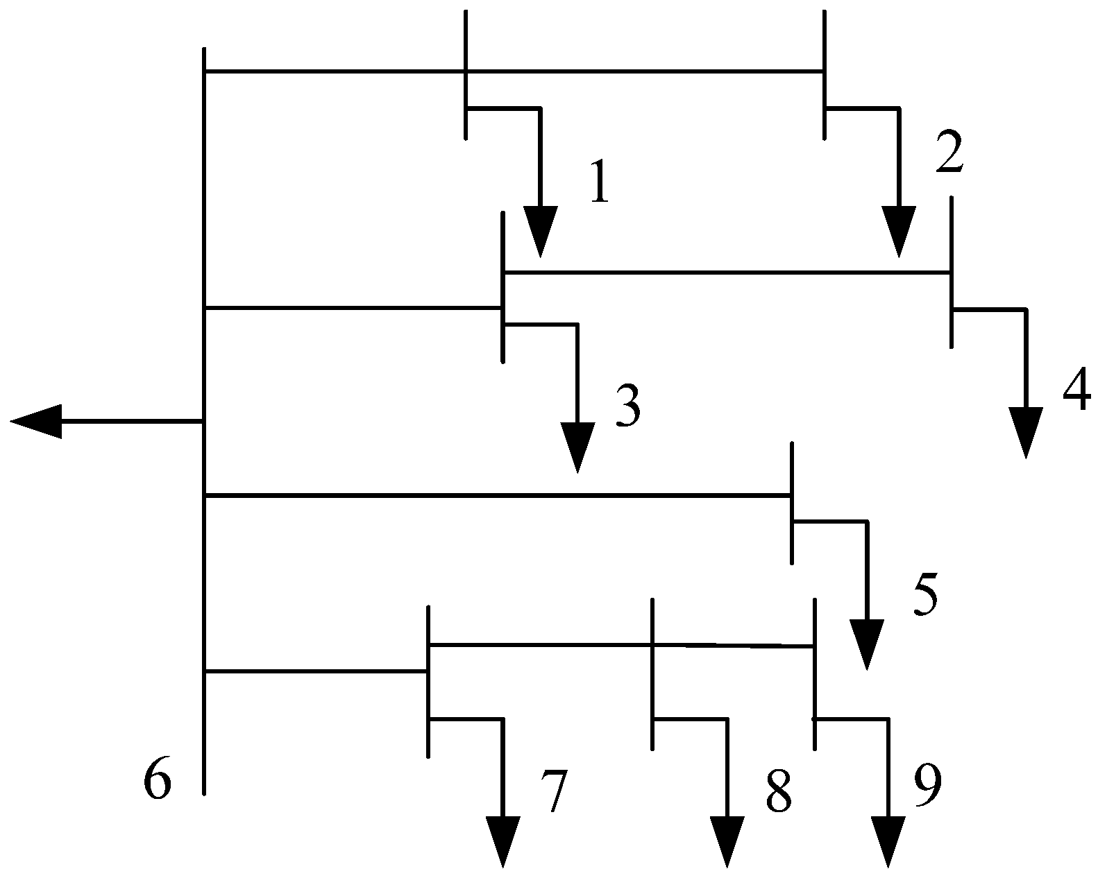
4. Case Study


| Node No. | 1 | 2 | 3 | 4 | 5 | 6 | 7 | 8 | 9 |
|---|---|---|---|---|---|---|---|---|---|
| Forecasted Power at jth hour (MW) | −0.107 | −0.1 | 0.1 | −0.2 | −0.3 | 0.46 | 0.1 | 0.1 | −0.105 |
| Line | Node i | 6 | 1 | 6 | 3 | 6 | 6 | 7 | 8 |
|---|---|---|---|---|---|---|---|---|---|
| Node j | 1 | 2 | 3 | 4 | 5 | 7 | 8 | 9 | |
| Length (km) | 1 | 6 | 3 | 7 | 12 | 5 | 3.5 | 5 | |
| Name | Price | |
|---|---|---|
| Fuel/Energy | Natural gas | ¥2.05/m3 |
| H2 | ¥160.00/40 L(12.8 MPa) | |
| O2 | ¥15.00/40 L(12.8 MPa) | |
| Selling | Busy time | ¥0.83/kWh |
| Normal time | ¥0.49/kWh | |
| spare time | ¥0.17/kWh | |
| Purchasing | Busy time | ¥0.65/kWh |
| Normal time | ¥0.38/kWh | |
| spare time | ¥0.13/kWh |


| Areas | Level 1 | Level 2 | Level 3 | Min |
|---|---|---|---|---|
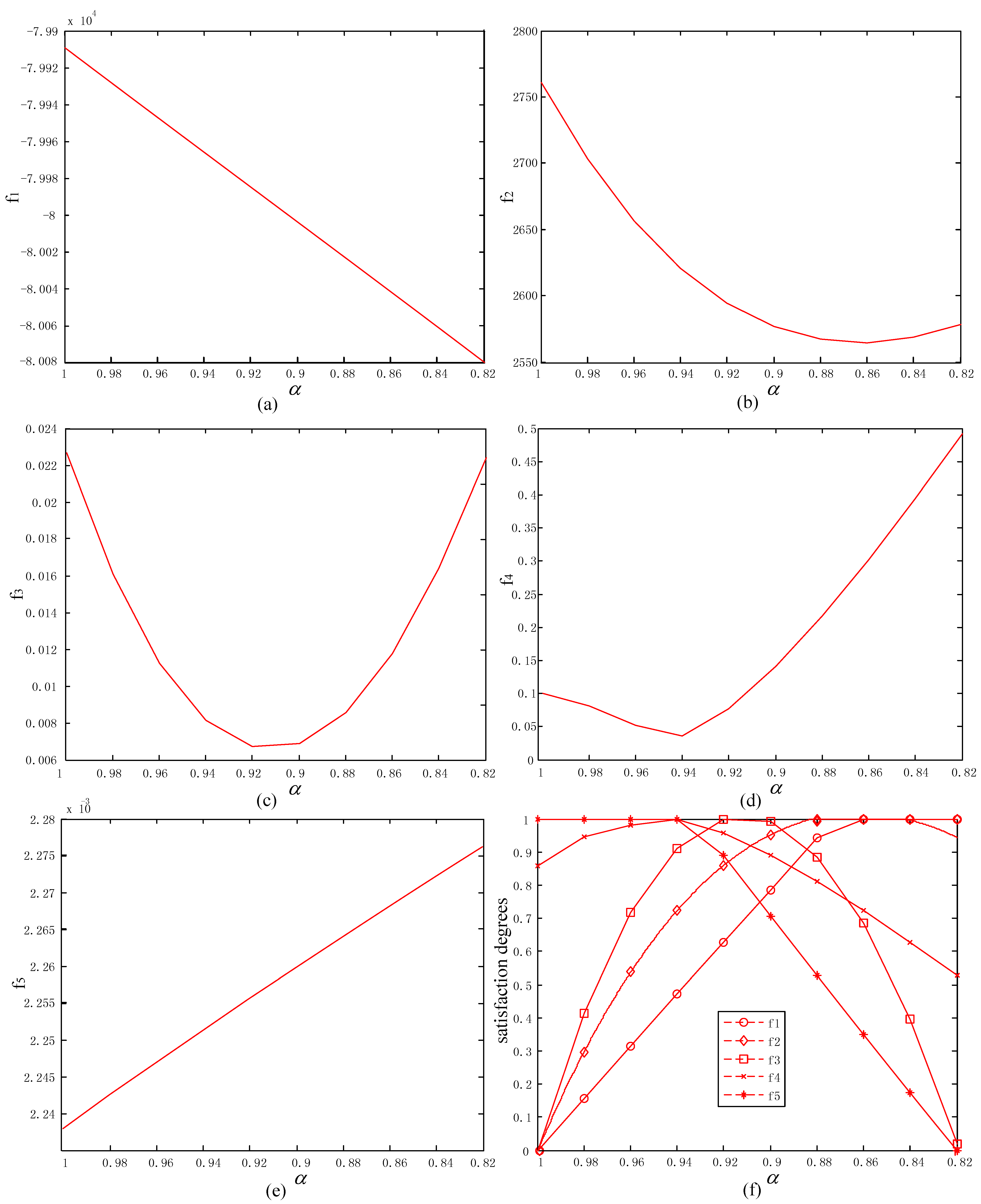
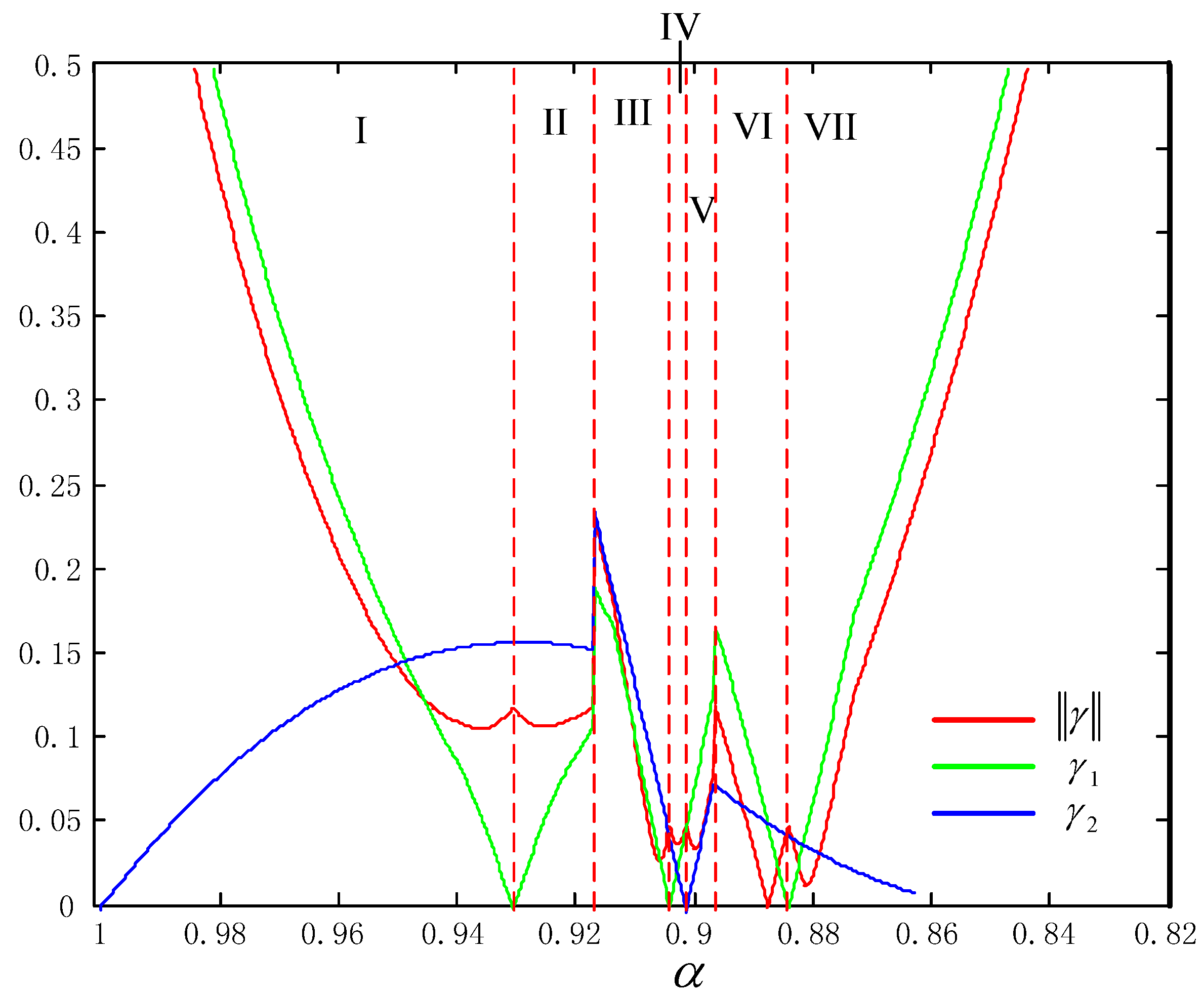
| I | f5 f4 | f3 f2 | f1 | 0.1077 |
| II | f5 f3 | f4 f2 | f1 | 0.1086 |
| III | f3 f5 | f2 f4 | f1 | 0.0282 |
| IV | f3 f2 | f5 f4 | f1 | 0.0384 |
| V | f3 f2 | f5 f1 | f4 | 0.0356 |
| VI | f2 f3 | f1 f5 | f4 | 0.0014 |
| VII | f2 f1 | f3 f5 | f4 | 0.0134 |
- Level 1: f3 and f2;
- Level 2: f4 and f5;
- Level 3: f1.
- k: k1 = 0.05, k2 = 0.05
| Bus No. | 1 | 2 | 3 | 4 | 5 | 6 | 7 | 8 | 9 |
|---|---|---|---|---|---|---|---|---|---|
| V (p.u.) | 0.9866 | 0.9915 | 1.0032 | 0.9672 | 1.0310 | 0.9998 | 1.0475 | 1.0391 | 0.9971 |
| Ang. (Rad.) | −0.0339 | −0.1486 | −0.0556 | −0.2886 | −0.6078 | −0.0009 | 0.0427 | 0.0327 | −0.0123 |
5. Conclusions
Acknowledgements
References
- Bignucolo, F.; Caldon, R.; Prandoni, V.; Spelta, S.; Vezzola, M. The Voltage Control on MV Distribution Networks with Aggregated DG Units (VPP). In Proceedings of the 41st International Universities Power Engineering Conference, Newcastle-Upon-Tyne, UK, 6–8 September 2006; Volume 1, pp. 187–192.
- Provoost, F.; Myrzik, J.M.A.; Kling, W.L. Optimizing LV Voltage Profile by Intelligent MV Control in Autonomously Controlled Networks. In Proceedings of the 41st International Universities Power Engineering Conference, Newcastle-Upon-Tyne, UK, 6–8 September 2006; Volume 1, pp. 354–358.
- Pudjianto, D.; Ramsay, C.; Strbac, G. Virtual power plant and system integration of distributed energy resources. IET Renew. Power Gener. 2007, 1, 10–16. [Google Scholar] [CrossRef]
- Bakari, K.E.; Kling, W.L. Virtual Power Plants: An Answer to Increasing Distributed Generation. In Proceedings of Innovative Smart Grid Technologies Conference Europe, Gotheburg, Sweden, 10–13 October 2010; pp. 1–6.
- Lukovic, S.; Kaitovic, I.; Mura, M.; Bondi, U. Virtual Power Plant as a Bridge between Distributed Energy Resources and Smart Grid. In Proceedings of 43rd Hawaii International Conference on System Sciences, Koloa, Kauai, HI, USA, 5–8 January 2010; pp. 1–8.
- EI Bakari, K.; Myrzik, J.M.A.; Kling, W.L. Prospects of a Virtual Power Plant to Control a Cluster of Distributed Generation and Renewable Energy Sources. In Proceedings of the 44th International Universities Power Engineering Conference, Glasgow, Scotland, 1–4 September 2009; pp. 1–5.
- Braun, M. Virtual Power Plant Functionalities Demonstrations in a Large Laboratory for Distributed Energy Resources. In Proceedings of 20th International Conference and Exhibition on Electricity Distribution—Part 1, Prague, Czech Republic, 8–11 June 2009; pp. 1–4.
- Salmani, M.A.; Anzalchi, A.; Salmani, S. Virtual Power Plant: New Solution for Managing Distributed Generations in Decentralized Power Systems. In Proceedings of International Conference on Management and Service Science, Wuhan, China, 24–26 August 2010; pp. 1–6.
- Caldon, R.; Patria, A.R.; Turri, R. Optimisation Algorithm for a Virtual Power Plant Operation. In Proceedings of 39th International Universities Power Engineering Conference, Bristol, UK, 6–8 September 2004; Volume 3, pp. 1058–1062.
- Salmani, M.A.; Tafreshi, S.M.M.; Salmani, H. Operation Optimization for a Virtual Power Plant. In Proceedings of IEEE PES/IAS Conference on Sustainable Alternative Energy, Valencia, Spain, 28–30 September 2009; pp. 1–6.
- Aggelogiannaki, E.; Sarimveis, H. A simulated annealing algorithm for prioritized multi-objective optimization-implementation in an adaptive model predictive control configuration. IEEE Trans. Syst. Man Cybern. 2007, 4, 902–915. [Google Scholar] [CrossRef]
- Palma-Behnke, R.; A, J.L.C.; Vargas, L.S.; Jofre, A. A distribution company energy acquisition market model with integration of distributed generation and load curtailment options. IEEE Trans. Power Syst. 2005, 4, 1718–1727. [Google Scholar] [CrossRef]
- Miettinnen, K. Nonlinear Multiobjective Optimization; Kluwer: Boston, MA, USA, 1999. [Google Scholar]
- Tiwari, R.N.; Dharmar, S.; Rao, J.R. Priority structure in fuzzy goal programming. Fuzzy Sets Syst. 1986, 19, 251–259. [Google Scholar] [CrossRef]
- Tao, Y.; Lv, X.Q.; Han, S.J.; Yang, W.L.; Zhang, X. Symmetrical Fuzzy Collaborative Optimization Using Satisficing and Sufficiency Degree Model. In Proceedings of 4th International Conference on Fuzzy Systems and Knowledge Discovery, Hainan, China, 24–27 August 2007; Volume 1, pp. 262–266.
- Chen, L.H.; Tsai, F.C. Fuzzy goal programming with different importance and priorities. Eur. J. Oper. Res. 2001, 133, 548–556. [Google Scholar] [CrossRef]
- Li, S.Y.; Hu, C.F. Two-step interactive satisfactory method for fuzzy multiple objective optimization with preemptive priorities. IEEE Trans. Fuzzy Syst. 2007, 15, 417–425. [Google Scholar] [CrossRef]
- Musio, M.; Lombardi, P.; Damiano, A. Vehicles to Grid (V2G) Concept Applied to a Virtual Power Plant Structure. In Proceedings of XIX International Conference on Electrical Machines (ICEM), Rome, Italy, 6–8 September 2010; pp. 1–6.
- Palma-Behnke, R.; Cerda, J.L.; Vargas, L.; Jofre, A. A distribution company energy acquisition market model with integration of distributed generation and load curtailment options. IEEE Trans. Power Syst. 2005, 20, 1718–1727. [Google Scholar] [CrossRef]
- de Brabandere, K.; Bolsens, B.; van den Keybus, J.; Woyte, A.; Driesen, J.; Belmans, R. A voltage and frequency droop control method for parallel inverters. IEEE Trans. Power Electron. 2007, 22, 1107–1115. [Google Scholar] [CrossRef]
- Ruiz, N.; Cobelo, I.; Oyarzabal, J. A direct load control model for virtual power plant management. IEEE Trans. Power Electron. 2009, 24, 959–966. [Google Scholar]
- Majumder, R.; Ghosh, A.; Ledwich, G.; Zare, F. Power management and power flow control with back-to-back converters in a utility connected microgrid. IEEE Trans. Power Electron. 2010, 25, 821–834. [Google Scholar]
- Teng, J.H. A direct approach for distribution system load flow solutions. IEEE Trans. Power Deliv. 2003, 18, 882–887. [Google Scholar] [CrossRef]
© 2011 by the authors; licensee MDPI, Basel, Switzerland. This article is an open access article distributed under the terms and conditions of the Creative Commons Attribution license (http://creativecommons.org/licenses/by/3.0/).
Share and Cite
Gong, J.; Xie, D.; Jiang, C.; Zhang, Y. Multiple Objective Compromised Method for Power Management in Virtual Power Plants. Energies 2011, 4, 700-716. https://doi.org/10.3390/en4040700
Gong J, Xie D, Jiang C, Zhang Y. Multiple Objective Compromised Method for Power Management in Virtual Power Plants. Energies. 2011; 4(4):700-716. https://doi.org/10.3390/en4040700
Chicago/Turabian StyleGong, Jinxia, Da Xie, Chuanwen Jiang, and Yanchi Zhang. 2011. "Multiple Objective Compromised Method for Power Management in Virtual Power Plants" Energies 4, no. 4: 700-716. https://doi.org/10.3390/en4040700
APA StyleGong, J., Xie, D., Jiang, C., & Zhang, Y. (2011). Multiple Objective Compromised Method for Power Management in Virtual Power Plants. Energies, 4(4), 700-716. https://doi.org/10.3390/en4040700