Evaluation of Lithium-Ion Battery Equivalent Circuit Models for State of Charge Estimation by an Experimental Approach

Abstract

To improve the use of lithium-ion batteries in electric vehicle (EV) applications, evaluations and comparisons of different equivalent circuit models are presented in this paper. Based on an analysis of the traditional lithium-ion battery equivalent circuit models such as the Rint, RC, Thevenin and PNGV models, an improved Thevenin model, named dual polarization (DP) model, is put forward by adding an extra RC to simulate the electrochemical polarization and concentration polarization separately. The model parameters are identified with a genetic algorithm, which is used to find the optimal time constant of the model, and the experimental data from a Hybrid Pulse Power Characterization (HPPC) test on a LiMn₂O₄ battery module. Evaluations on the five models are carried out from the point of view of the dynamic performance and the state of charge (SoC) estimation. The dynamic performances of the five models are obtained by conducting the Dynamic Stress Test (DST) and the accuracy of SoC estimation with the Robust Extended Kalman Filter (REKF) approach is determined by performing a Federal Urban Driving Schedules (FUDS) experiment. By comparison, the DP model has the best dynamic performance and provides the most accurate SoC estimation. Finally, sensitivity of the different SoC initial values is investigated based on the accuracy of SoC estimation with the REKF approach based on the DP model. It is clear that the errors resulting from the SoC initial value are significantly reduced and the true SoC is convergent within an acceptable error.

1. Introduction

With the increased research in the fields of hybrid electric vehicle dynamic simulation, energy distribution and power control strategy, as well as the estimation of batteries’ state of charge (SoC) and state of health (SoH) [1,2,3,4,5,6], nowadays improving the accuracy of the charging and discharging model of power batteries, especially lithium-ion batteries, is a significant objective.

Since the battery is a nonlinear system, the models usually used in electric vehicles (EVs) can be divided into three kinds: the simplified electrochemical model was proposed based on the electrochemical theory [7,8,9], and could fully describe the characteristics of the power battery by using mathematics to describe the inner action of the battery. For example, the Peukert equation can simply associate the power battery to an invariant linear system, however, it cannot handle its nonlinear characteristics and it can hardly simulate its dynamic performance.

In order to overcome the drawbacks of the mathematical models, the neural network model was put forward, which took the weights of neurons into account instead of the state variables [10,11,12,13,14]. The accuracy of this model could reach 3% under certain conditions. However, the accuracy and calculation burden of the model were influenced by the choices and quantity of input variables of the neural network. Also, a neural network trained by data can only be used within the original scope of that data.

Based on the dynamic characteristics and working principles of the battery, the equivalent circuit model was developed by using resistors, capacitors and voltage sources to form a circuit network [15,16,17]. Typically, a large capacitor or an ideal voltage source was selected to represent the open-circuit voltage (OCV), the remainder of the circuit simulated the battery’s internal resistance and dynamic effects such as terminal voltage relaxation. On a basis of the OCV estimate, SoC could be inferred via a lookup table. The equivalent circuit model has been widely used in various types of modeling and simulation for EVs and battery management systems. Evidently high dynamic simulation with high accuracy is one of the key technologies.

In this paper, a LiMn₂O₄ battery module with a nominal voltage of 57.6 V and a nominal capacity of 100 Ah is researched. An improved model is proposed based on the investigations of the traditional models from the point of view of the aspects of dynamic performance and SoC estimation. The model parameters are identified by the genetic algorithm along with the experimental data. The dynamic performances of the battery models are compared and the accuracy of the model-based SoC estimations with a robust extended Kalman filter (REKF) are evaluated. Furthermore, the sensitivity of the different SoC initial values on the presented model-based SoC estimation is discussed.

2. Equivalent Circuit Models of Lithium-Ion Battery

Various equivalent circuit models such as the Rint model, the RC model, the Thevenin model or the PNGV model are now widely used in EV studies [16,17,18]. In order to refine the polarization characteristics of a battery, an improved Thevenin circuit model named DP (for dual polarization) model is proposed herein. Further, comparisons between the model-based simulation data and the experimental data are carried out to evaluate the validity of the foregoing models, which provides a foundation for the model-based SoC estimation.

2.1. The Rint Model

The Rint model, as shown in Figure 1 and Equation (1), implements an ideal voltage source U_oc to define the battery open-circuit voltage. Both resistance R_o and open-circuit voltage U_oc are functions of SoC, SoH and temperature. I_L is load current with a positive value at discharging and a negative value at charging, U_L is the terminal voltage.

Figure 1. Schematic diagram of the Rint model.

Figure 1. Schematic diagram of the Rint model.

U_L = U_oc − I_LR_o

(1)

2.2. The RC Model

The RC model was designed by the famous SAFT Battery Company, and has achieved good application via the Advisor software. As shown in Figure 2, it consists of two capacitors (C_c, C_b) and three resistors (R_t, R_e, R_c). The capacitor C_c, which has a small capacitance and mostly represents the surface effects of a battery, is named surface capacitor. The capacitor C_b, which has a very large capacitance and represents the ample capability of a battery to store charge chemically, is named bulk capacitor. SoC can be determined by the voltage across the bulk capacitor. Resistors R_t, R_e, R_c are named terminal resistor, end resistor and capacitor resistor, respectively. U_b and U_c are the voltages across C_b and C_c, respectively. The electrical behaviour of the circuit can be expressed by Equations (2) and (3).

Figure 2. Schematic diagram of the RC model.

Figure 2. Schematic diagram of the RC model.

(2)

(3)

2.3. The Thevenin Model

The Thevenin model connects a parallel RC network in series based on the Rint model, describing the dynamic characteristics of the battery. As shown in Figure 3, it is mainly composed of three parts including open-circuit voltage U_oc, internal resistances and equivalent capacitances. The internal resistances include the ohmic resistance R_o and the polarization resistance R_Th. The equivalent capacitance C_Th is used to describe the transient response during charging and discharging. U_Th is the voltages across C_Th. I_Th is the outflow current of C_Th. The electrical behavior of the Thevenin model can be expressed by Equation (4).

Figure 3. Schematic diagram for the Thevenin model.

Figure 3. Schematic diagram for the Thevenin model.

$$\{\begin{array}{l}{\dot{U}}_{\text{Th}}=-\frac{U_{\text{Th}}}{R_{\text{Th}}{C}_{\text{Th}}}+\frac{I_{\mathrm{L}}}{C_{\text{Th}}}\hfill \\ U_{\mathrm{L}}=U_{\text{oc}}-U_{\text{Th}}-I_{\mathrm{L}}{R}_{\mathrm{o}}\hfill \end{array}$$

(4)

2.4. The PNGV Model

The PNGV model as shown in Figure 4 can be obtained by adding a capacitor $1/U_{\text{oc}}^{\prime }$ in series based on the Thevenin model to describe the changing of open circuit voltage generated in the time accumulation of load current.

Figure 4. Schematic diagram of the PNGV model.

Figure 4. Schematic diagram of the PNGV model.

U_d and U_PN are the voltages across $1/U_{\text{oc}}^{\prime }$ and C_PN respectively. I_PN is the outflow current of C_PN. The electrical behavior of the PNGV model can be expressed by Equation (5):

$$\{\begin{array}{l}{\dot{U}}_{\mathrm{d}}=U_{\mathrm{oc}}^{\prime }{I}_{\mathrm{L}}\hfill \\ {\dot{U}}_{\text{PN}}=\frac{U_{\text{PN}}}{R_{\text{PN}}{C}_{\text{PN}}}+\frac{I_{\mathrm{L}}}{C_{\text{PN}}}\hfill \\ U_{\mathrm{L}}=U_{\text{oc}}-U_{\mathrm{d}}-U_{\text{PN}}-I_{\mathrm{L}}{R}_{\mathrm{o}}\hfill \end{array}$$

(5)

2.5. The DP Model

Based on the test analysis of the characteristics of a lithium-ion power battery, an obvious polarization can be observed. The polarization characteristic could be simulated by the Thevenin model to some extent, however, the difference between concentration polarization and electrochemical polarization leads to an inaccurate simulation in the moments at the end of charge or discharge. An improved circuit model is presented in Figure 5, which is defined as dual polarization (DP) model, to refine the description of polarization characteristics and simulate the concentration polarization and the electrochemical polarization separately.

Figure 5. Schematic diagram for the DP model.

Figure 5. Schematic diagram for the DP model.

The DP model the composed of three parts: (1) Open-circuit voltage U_oc; (2) Internal resistances such as the ohmic resistance R_o and the polarization resistances, which include R_pa to represent the effective resistance characterizing electrochemical polarization and R_pc to represent the effective resistance characterizing concentration polarization; (3) the effective capacitances like C_pa and C_pc, which are used to characterize the transient response during transfer of power to/from the battery and to describe the electrochemical polarization and the concentration polarization separately. U_pa and U_pc are the voltages across C_pa and C_pc respectively. I_pa and I_pc are the outflow currents of C_pa and C_pc respectively. The electrical behavior of the circuit can be expressed by Equation (6):

$$\{\begin{array}{l}{\dot{U}}_{\text{pa}}=-\frac{U_{\text{pa}}}{R_{\text{pa}}{C}_{\text{pa}}}+\frac{I_{\mathrm{L}}}{C_{\text{pa}}}\hfill \\ {\dot{U}}_{\text{pc}}=\frac{U_{\text{pc}}}{R_{\text{pc}}{C}_{\text{pc}}}+\frac{I_{\mathrm{L}}}{C_{\text{pc}}}\hfill \\ U_{\mathrm{L}}=U_{\text{oc}}-U_{\text{pa}}-U_{\text{pc}}-I_{\mathrm{L}}{R}_{\mathrm{o}}\hfill \end{array}$$

(6)

3. Model Parameters’ Identification of a Lithium-Ion Power Battery Module

To identify the model parameters, a battery test bench is designed. The purpose of recognition is based on a criterion and the measurement information of the known systems to estimate the model structure and unknown parameters.

3.1. Battery Test Bench

The configuration of the battery test bench is shown in Figure 6. The key equipment is the Digatron EVT500-500, which can charge/discharge battery module with a maximum voltage of 500 V and a maximum current of 500 A, and can measure in a timely fashion the major parameters like voltage, current and temperature. The host computer with the installed BTS-600 software can program the experimental procedures and deal with real-time data acquisition. In order to limit the temperature’s influence on the model parameters, all of the experiments of the LiMn₂O₄ battery module are carried out in a thermal chamber with a fixed temperature of 20 °C.

Figure 6. Configuration of the battery test bench.

Figure 6. Configuration of the battery test bench.

3.2. Experimental Design

In order to acquire data to identify the model parameters, a Hybrid Pulse Power Characterization (HPPC) [17] test procedure is conducted on the LiMn₂O₄ battery module at 0.1 SoC intervals (constant current C/3 discharge segments) starting from 1.0 to 0.1 and each interval followed by a 2-hour rest to allow the battery to get an electrochemical and thermal equilibrium condition before applying the next.

Figure 7. The terminal voltage profile at SoC = 0.1 during the HPPC test.

Figure 7. The terminal voltage profile at SoC = 0.1 during the HPPC test.

Figure 7 shows the terminal voltage profile of the battery module at SoC = 0.1 during the HPPC test. It is assumed that the current is (+)ve when the battery discharges and (−)ve when the battery charges.

3.3. Model Parameters’ Identification Method

3.3.1. The Rint Model

Based on the experimental data, a regression analysis according to Equation (1) with the input of I_L is conducted at each SoC separately. A confirmed coefficient r², which is defined as Equation (7), is selected to evaluate the identification accuracy:

$$r^2=\frac{{\displaystyle \sum {({\widehat{U}}_{\mathrm{L}}-{\stackrel{-}{U}}_{\mathrm{L}})}^2}}{{\displaystyle \sum {(U_{\mathrm{L}}-{\stackrel{-}{U}}_{\mathrm{L}})}^2}}$$

(7)

where ${\widehat{U}}_{\mathrm{L}}$ is the model-based observer value of U_L, ${\stackrel{-}{U}}_{\mathrm{L}}$ is the average value of U_L.

3.3.2. The RC Model

According to the method provided in the guide document of ADVISOR [16], the HPPC test data is used to identify the five unknown parameters (C_c, C_b, R_t, R_e, R_c) at each SoC separately.

3.3.3. The Thevenin Model

In order to identify the model parameters, a regression equation is built as Equation (8). The appropriate time constant of polarization (τ_Th = R_ThC_Th) needs to be given in advance based on the battery characteristics:

(8)

In this paper, a genetic algorithm is used to find the optimal value of τ_Th and the objective function of the genetic algorithm is built as follows:

(9)

where, ${\widehat{\mathrm{\chi }}}_{\mathrm{k}}^{(\mathrm{g})}$ is the estimation value of current population χ_k at generation g; χ_k is the current individual k of the population χ, where χ = [τ_Th]; ${\widehat{U}}_{\text{L,k}}$ is the estimation value of U_L at the individual k; N is the estimation length, here N = 200.

3.3.4. The PNGV Model

The model parameters’ identification of the PNGV model with regression Equation (10) is similar to that of the Thevenin model, and it also needs to pre-set the time constant τ_PN. The same genetic algorithm as Equation (9) where χ=[τ_PN] was used to find the optimal value of τ_PN:

(10)

3.3.5. The DP Model

The model parameters’ identification of the DP model with regression Equation (11) is similar to that of the Thevenin model, and it also needs to pre-set time constants τ_pc and τ_pa. The same genetic algorithm as Equation (9), where $\mathbf{\chi }=\left[\begin{array}{ll}{\tau }_{\text{pa}}\hfill & 0\hfill \\ 0\hfill & {\tau }_{\text{pc}}\hfill \end{array}\right]$ is used to find the optimal values of τ_pc and τ_pa:

(11)

3.4. Identification Results

The identification results of the Rint model, the RC model, the Thevenin model, the PNGV model and the DP model for the SoC within the ranges of 0.5 and 0.6 are shown in Table 1, Table 2, Table 3, Table 4 and Table 5, respectively.

Table 1. The identification results of the Rint model.

SoC	r2	Uoc (V)	Ro (Ω)
0.5	0.996	63.158	0.02486
0.6	0.997	63.676	0.02465

Table 1. The identification results of the Rint model.

SoC	r2	Uoc (V)	Ro (Ω)
0.5	0.996	63.158	0.02486
0.6	0.997	63.676	0.02465

Table 2. The identification results of the RC model.

SoC	r2	Cb (F)	Re (Ω)	Cc (F)	Rc (Ω)	Rt (Ω)
0.5	0.976	58103	0.01776	24.73	0.00651	0.01954
0.6	0.982	70266	0.01776	27.60	0.00651	0.01954

Table 2. The identification results of the RC model.

SoC	r2	Cb (F)	Re (Ω)	Cc (F)	Rc (Ω)	Rt (Ω)
0.5	0.976	58103	0.01776	24.73	0.00651	0.01954
0.6	0.982	70266	0.01776	27.60	0.00651	0.01954

Table 3. The identification results of the Thevenin model.

SoC	r2	Uoc (V)	CTh (F)	RTh (Ω)	Ro (Ω)	τTh (s)
0.5	0.999	63.294	4581	0.007360	0.02423	33.7
0.6	0.999	63.808	5141	0.007046	0.024223	34.2

Table 3. The identification results of the Thevenin model.

SoC	r2	Uoc (V)	CTh (F)	RTh (Ω)	Ro (Ω)	τTh (s)
0.5	0.999	63.294	4581	0.007360	0.02423	33.7
0.6	0.999	63.808	5141	0.007046	0.024223	34.2

Table 4. The identification results of the PNGV model.

SoC	r2	Uoc (V)	$1/U_{\mathrm{oc}}^{\prime }$ (F)	CPN (F)	RPN (Ω)	Ro (Ω)	τPN (s)
0.5	0.999	63.327	8373761	4643	0.00719	0.02425	33.4
0.6	0.999	63.845	8597339	4635	0.00678	0.02424	34.5

Table 4. The identification results of the PNGV model.

SoC	r2	Uoc (V)	$1/U_{\mathrm{oc}}^{\prime }$ (F)	CPN (F)	RPN (Ω)	Ro (Ω)	τPN (s)
0.5	0.999	63.327	8373761	4643	0.00719	0.02425	33.4
0.6	0.999	63.845	8597339	4635	0.00678	0.02424	34.5

Table 5. The identification results of the DP model.

SoC	r2	Uoc	Cpa	Rpa	Cpc	Rpc	Ro	τpa	τpc
0.5	0.999	63.302	5630	0.00064	54277	0.00824	0.02402	3.6	44.7
0.6	0.999	63.824	5700	0.00065	53817	0.00839	0.02406	3.7	45.2

Table 5. The identification results of the DP model.

SoC	r2	Uoc	Cpa	Rpa	Cpc	Rpc	Ro	τpa	τpc
0.5	0.999	63.302	5630	0.00064	54277	0.00824	0.02402	3.6	44.7
0.6	0.999	63.824	5700	0.00065	53817	0.00839	0.02406	3.7	45.2

There is no similarity between Table 2 and the other four tables due to the totally different model structures of the RC model. The other four tables show the model parameters, U_oc and R_o are similar, but those parameters identifying the polarization characteristics are totally different due to the different levels of description of the polarization characteristics.

4. Evaluation on the Lithium-Ion Battery Models

4.1. Model Verification

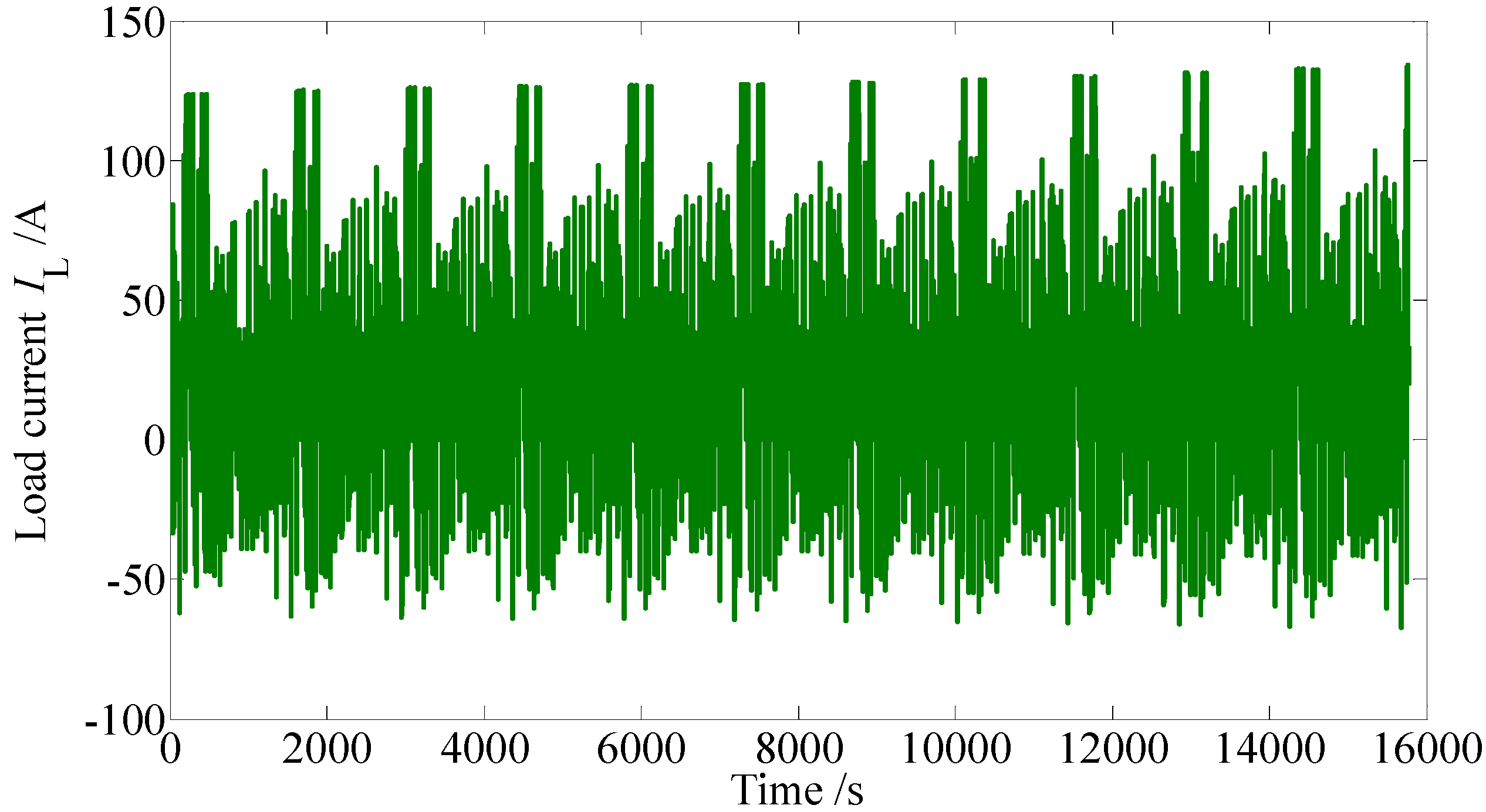
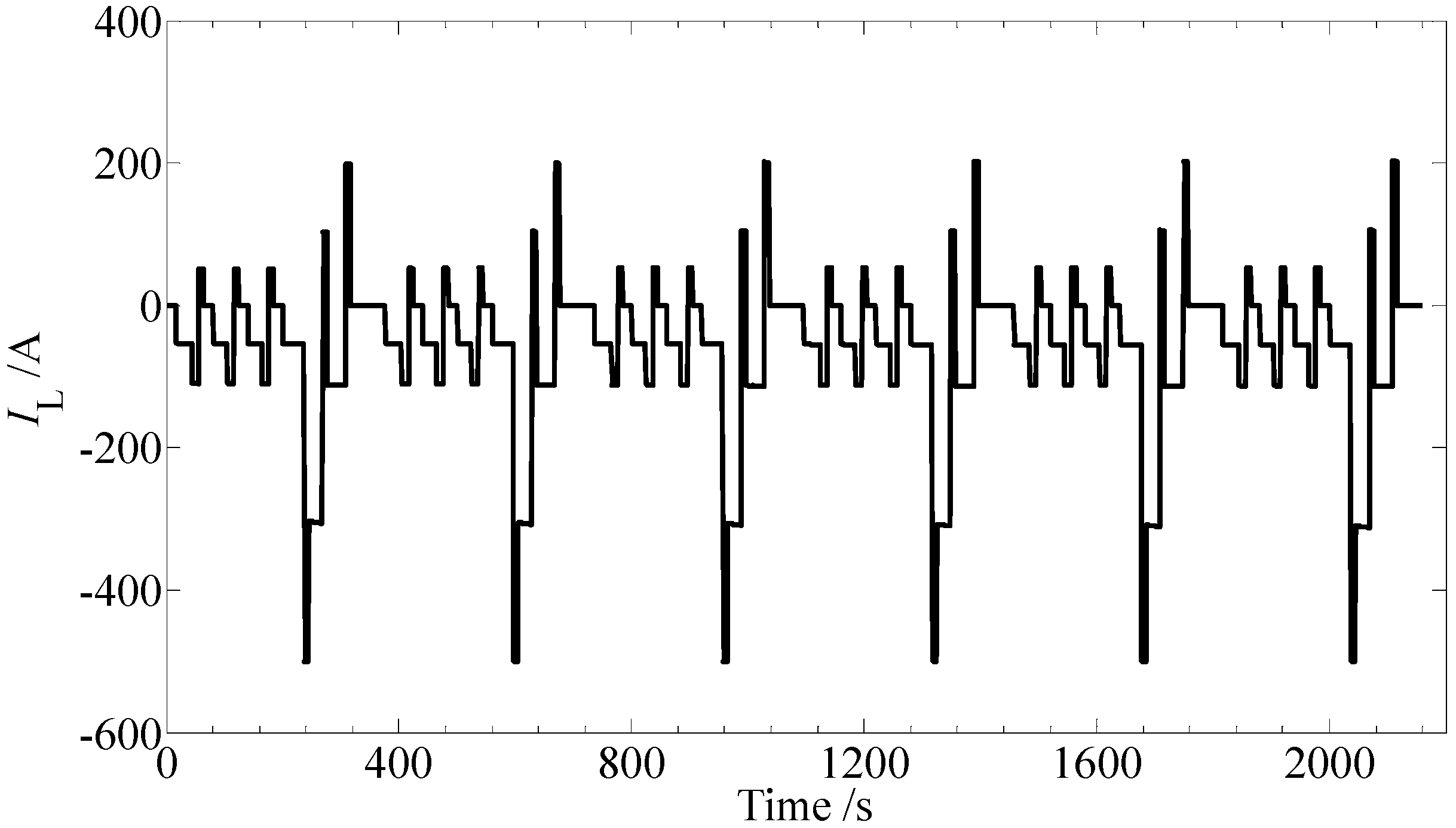
To evaluate the validity of the battery models, six consecutive Dynamic Stress Test (DST) cycles [16] which is a standard testing program of the EVT500-500, are adopted as the input for both the lithium-ion battery module and the battery models, as shown in Figure 8. The initial SoC is 100%. The parameters of the battery models as a function of SoC are updated via linear lookup table and extrapolation.

Figure 8. The load current profiles of 6 DST testing cycles.

Figure 8. The load current profiles of 6 DST testing cycles.

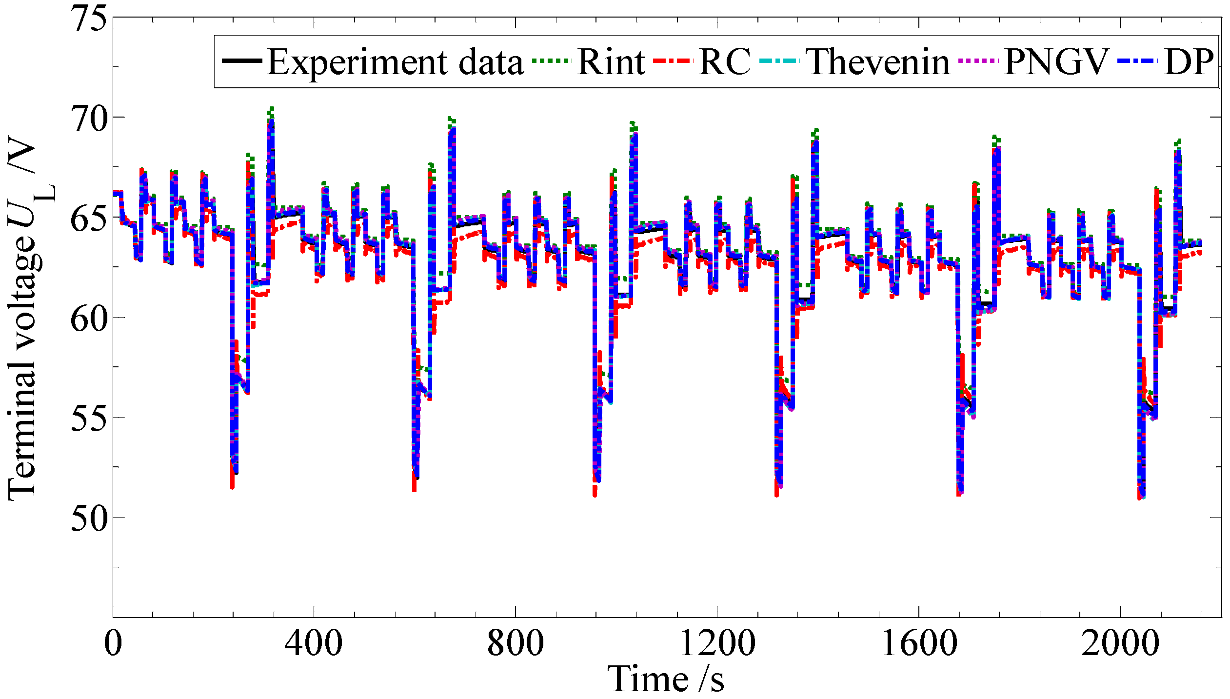
Figure 9 presents the terminal voltage curves of the experimental data and the model-based simulation data.

Figure 9. The terminal voltage profiles of the model-based simulation and experiment.

Figure 9. The terminal voltage profiles of the model-based simulation and experiment.

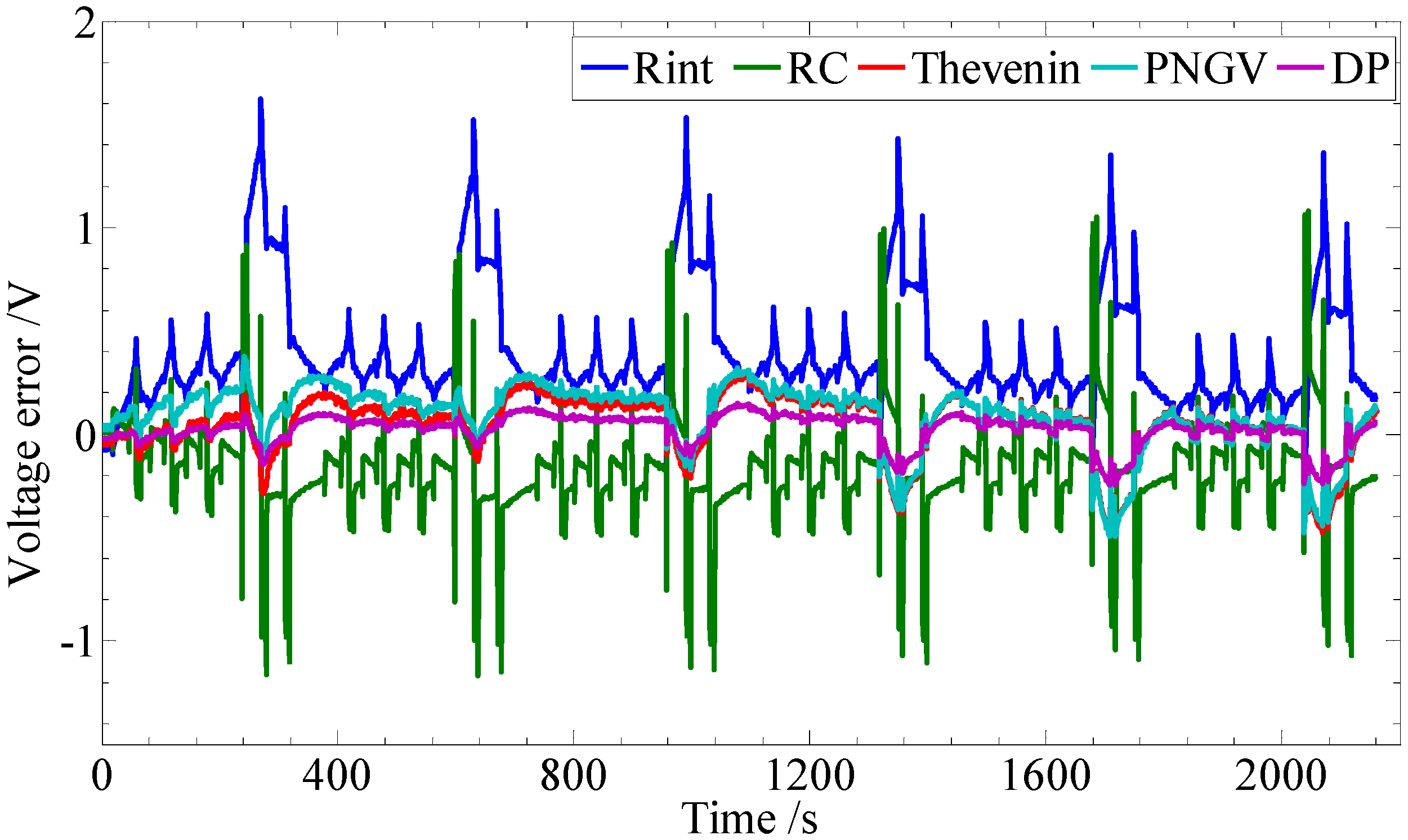
The comparison curves of the terminal voltage between the experimental data and the model-based simulation data are drawn as shown in Figure 10.

Figure 10. The terminal voltage error curves between the simulation and experiment.

Figure 10. The terminal voltage error curves between the simulation and experiment.

It can be concluded that all five equivalent circuit models simulate the dynamic characteristics to some extent, albeit with different accuracy. Both the DP model and the Thevenin model have better dynamic simulation results, which indicates that these two models are more suitable for the modeling of lithium-ion batteries.

4.2. Evaluation on the Accuracy of the Battery Models

A statistical analysis on the absolute values of the terminal voltage errors was conducted and the results were as shown in Table 6. It shows that the Rint model has the biggest error and can hardly simulate the dynamic performance of the power battery since the polarization characteristic has been ignored. The PNGV model and the Thevenin model can both simulate the polarization characteristics. Compared with the Thevenin model, the PNGV model has an additional capacitor which accounts for the influence of the open circuit voltage. However, it will produce a fluctuation in the battery model, and causes a big error. The terminal voltage estimated by the Thevenin model has a better dynamic performance following the experimental data, and its maximum error rate is less than 1%. The big error caused by the RC model also indicates that it needs much improvement and optimization. With regard to the DP model, it can simulate the battery with better dynamic characteristics as well as the smallest error compared with other models, so by comparison, the DP model is both accurate and reasonable.

Table 6. The statistic analysis list of the absolute values of terminal voltage errors.

Model	Maximum (V)	Mean (V)	Variance (V2)	Max. Error Rate (%)
Rint model	1.6229	0.3945	0.0762	2.8176
RC model	1.0785	0.2336	0.0463	2.0337
Thevenin model	0.2967	0.0455	0.0220	0.5151
PNGV model	0.5772	0.0875	0.0243	1.0020
DP model	0.2183	0.0429	0.0021	0.3790

Table 6. The statistic analysis list of the absolute values of terminal voltage errors.

Model	Maximum (V)	Mean (V)	Variance (V2)	Max. Error Rate (%)
Rint model	1.6229	0.3945	0.0762	2.8176
RC model	1.0785	0.2336	0.0463	2.0337
Thevenin model	0.2967	0.0455	0.0220	0.5151
PNGV model	0.5772	0.0875	0.0243	1.0020
DP model	0.2183	0.0429	0.0021	0.3790

4.3. Evaluation on the Adaptability of the Battery Models for SoC Estimation

The Federal Urban Driving Schedules (FUDS) is a typical driving cycle which is often used to evaluate various SoC estimation algorithms. In this paper, eleven consecutive FUDS were employed to verify the SoC estimation approach, and the sampled current profiles are shown in Figure 11.

Figure 11. Load Current profile sampled during eleven consecutive FUDS cycles.

Figure 11. Load Current profile sampled during eleven consecutive FUDS cycles.

The model-based SoC estimation greatly depends on the algorithms and this may lead to a fluctuant, even divergent result. The Kalman filter algorithm can reduce the fluctuation by adjusting the gain matrix based on the error between the model-observed value and the actual value of the terminal voltage, and gradually make the SoC estimation approach the true value. Meanwhile, another feature of the Kalman filter is its strong dependence on the model accuracy [14,16]. In order to reduce the dependence of the Kalman filter on uncertain factors, a robust extended Kalman filter (REKF) algorithm is selected and designed for the implementation of the SoC estimation [19,20].

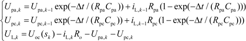
The SoC estimations with REKF algorithm were conducted for the five models. A detailed description with the DP model taken as an example follows:

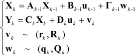
The state equation and observation equation of the discrete system of interest with REKF algorithm is as follows:

(12)

where X is a n × 1 state matrix; Y is a m × 1 observe matrix; A, B, C, D and Γ are n × n, n × 1, m × n, m × 1 and n × n matrix respectively; w_k is a process noise with mean of q_k and covariance of Q_k; v_k is the measurement noise with mean of r_k and covariance of R_k

Transform the Equation (6) to a discrete system:

(13)

Define state matrix X and SoC as:

$$\mathbf{X}=\left\{\begin{array}{c}{U}_{\text{pa}}\\ U_{\text{pc}}\\ s\end{array}\right\}$$

(14)

$$s_k=s_{k-1}-\frac{\eta I_{\mathrm{L},k}\Delta t}{C_N}$$

(15)

Then, the matrix A, B, C and D can be written as follows:

$${\mathbf{A}}_{k-1}=\left(\begin{array}{ccc}\exp (-\Delta t/(R_{\text{pa}}{C}_{\text{pa}}))& 0& 0\\ 0& \exp (-\Delta t/(R_{\text{pc}}{C}_{\text{pc}}))& 0\\ 0& 0& 1\end{array}\right)$$

(16)

$${\mathbf{B}}_{\mathrm{k}-1}=\left(\begin{array}{c}{R}_{\text{pa}}(1-\exp (-\Delta t/(R_{\text{pa}}{C}_{\text{pa}})))\\ R_{\text{pc}}(1-\exp (-\Delta t/(R_{\text{pc}}{C}_{\text{pc}})))\\ \eta \Delta t/C_{\text{N}}\end{array}\right)$$

(17)

$${\mathbf{C}}_{k-1}=\frac{\partial U_L}{{\partial }_{\mathbf{X}}}{|}_{\mathbf{X}={\widehat{\mathbf{X}}}_{k-1}}=\left[\begin{array}{ccc}-1& -1& \frac{\mathrm{d}{U}_{\mathrm{o}\mathrm{c}}(s)}{\mathrm{d}s}\end{array}\right]$$

(18)

D_k−1 = [R_o]

(19)

Y_k = [U_L,k]

(20)

where, s is the abbreviation of SoC, Δt is the sample step, η is the coulombic efficiency, C_N is the nominal capacity of the battery.

The experimental data of the coulombic efficiency under different charging/discharging current for the lithium-ion battery module are shown in Table 7, which shows that the coulombic efficiency decreases with the increase of the discharge current and it is necessary to limit the discharge current range for a higher efficiency.

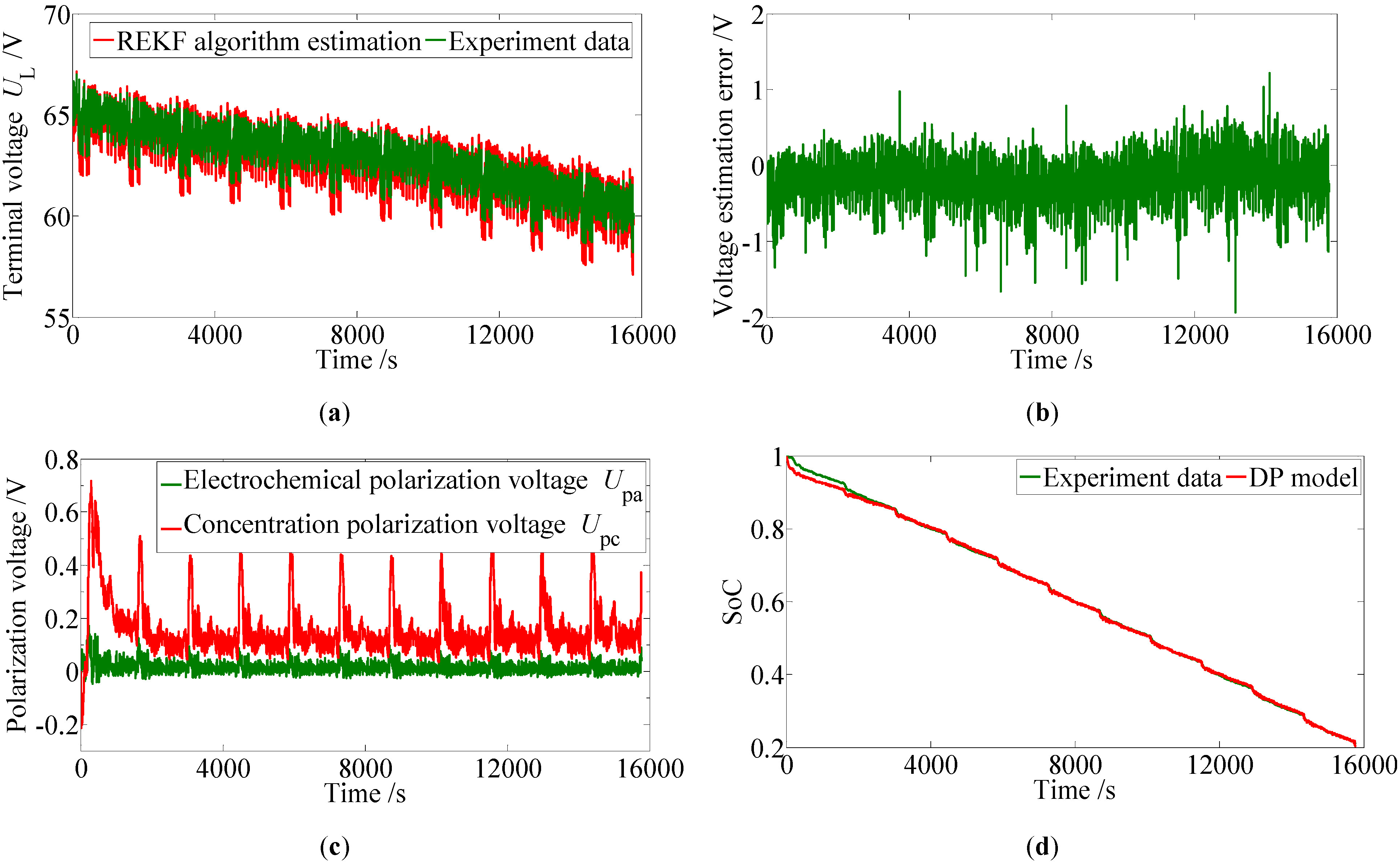
Set the initial values as: X₀ = [0 0 1]^T; R = 10; Q = diag (0.00001, 0.00001, 0.00001, 0.00001, 0.00001); P₀ = diag (1, 0.1, 0.1, 0.1, 0.1) (herein, P is the covariance matrix of X). The DP model-based SoC estimation results with REKF are shown in Figure 12.

Table 7. Coulombic efficiency list of the lithium-ion battery module.

Current (A)	30	50	100	150	200	300
Coulombic efficiency in discharging process (%)	100	99.3	98.5	98.1	97.4	95.2
Coulombic efficiency in charging process (%)	100	98.5	97.4	96.0	94.0	-

Table 7. Coulombic efficiency list of the lithium-ion battery module.

Current (A)	30	50	100	150	200	300
Coulombic efficiency in discharging process (%)	100	99.3	98.5	98.1	97.4	95.2
Coulombic efficiency in charging process (%)	100	98.5	97.4	96.0	94.0	-

Figure 12. The DP model-based SoC estimation results with REKF: (a) Terminal voltage; (b) Voltage estimation error; (c) Polarization voltages; (d) SoC.

Figure 12. The DP model-based SoC estimation results with REKF: (a) Terminal voltage; (b) Voltage estimation error; (c) Polarization voltages; (d) SoC.

4.3.1. SoC Estimation Accuracy

Figure 12(d) shows the experimental SoC data based on the Digatron EVT 500-500 test bench results after proper adjustments as follows: in order to get the true SoC by an experimental approach, firstly, the battery module is fully charged to make sure the initial SoC is 1.0; after the eleven consecutive FUDS test is finished, the battery module is rested for at least 2 hours and a further discharge experiment with nominal current is conducted until the battery module is fully discharged, and then the true value of the terminal SoC can be calculated according to the definition of SoC. Since the true values of the initial SoC and the terminal SoC are determined, the simple Ah counting method is used to calculate the experimental SoC based on the load current profile and the coulomb efficiency map, also a proper adjustment coefficient, which is calculated based on the true values of the initial SoC and terminal SoC, is applied during the calculation. The Ah counting method with an adjustment approach based on a further discharging experiment can only be used in laboratory. Herein, it is used to provide a true SoC profile for comparison purposes. 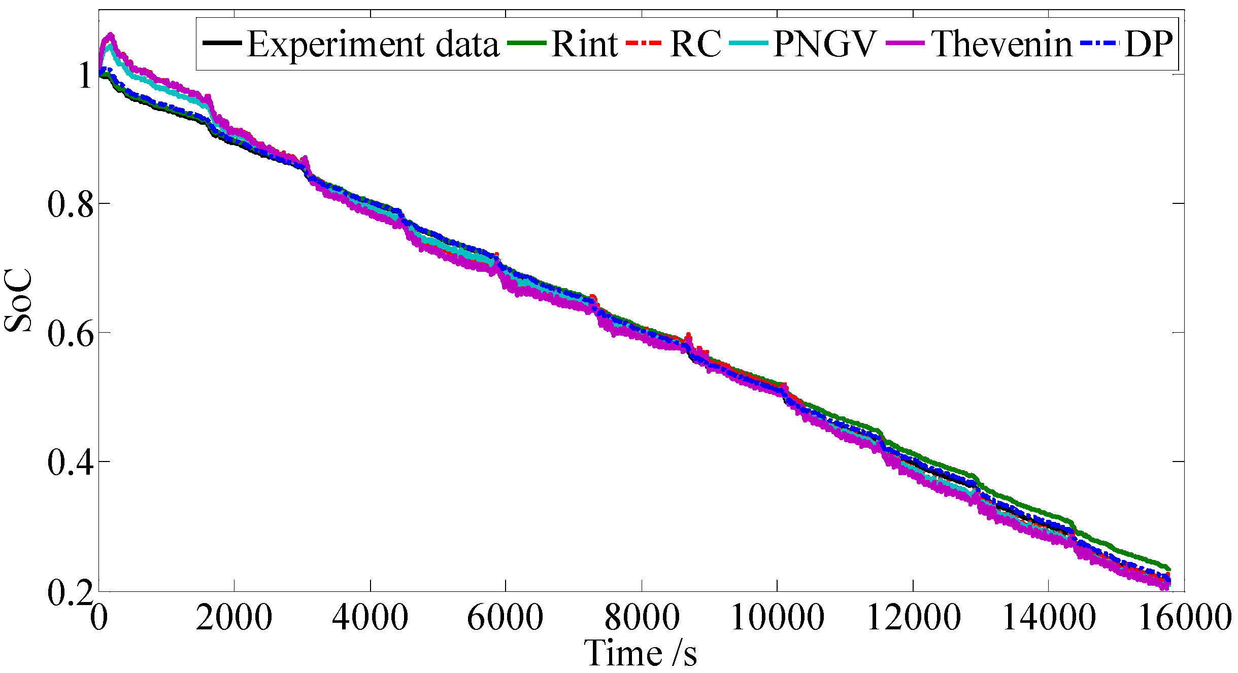The results of the SoC estimation with REKF for the five models are shown in Figure 13 and the comparisons between the estimations and the experiment are shown in Figure 14. A statistic analysis on the absolute SoC estimation errors is conducted and the results including the terminal SoC error are list in Table 8.

Figure 13. SoC estimation profiles based on FUDS cycles.

Figure 13. SoC estimation profiles based on FUDS cycles.

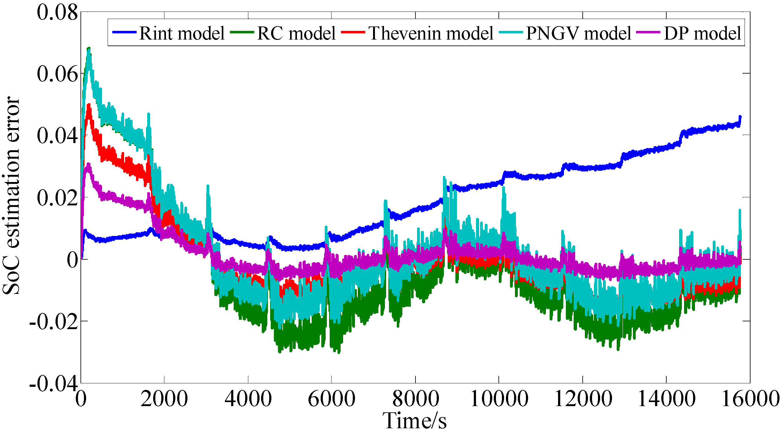
Figure 14. The SoC estimation error profiles based on FUDS cycles.

Figure 14. The SoC estimation error profiles based on FUDS cycles.

Table 8. The statistic list of the absolute SoC estimation error and the terminal SoC error.

Model	Maximum	Mean	Variance	Terminal
Rint Model	0.0462	0.0186	0.0012	0.046
RC Model	0.0681	0.0167	0.0009	0.013
Thevenin Model	0.0500	0.0101	0.0004	−0.016
PNGV Model	0.0675	0.0126	0.0005	−0.017
DP Model	0.0309	0.0047	0.00004	−0.005

Table 8. The statistic list of the absolute SoC estimation error and the terminal SoC error.

Model	Maximum	Mean	Variance	Terminal
Rint Model	0.0462	0.0186	0.0012	0.046
RC Model	0.0681	0.0167	0.0009	0.013
Thevenin Model	0.0500	0.0101	0.0004	−0.016
PNGV Model	0.0675	0.0126	0.0005	−0.017
DP Model	0.0309	0.0047	0.00004	−0.005

According to Figure 14 and Table 8, it can be seen that for the Rint model, due to the precise initial SoC and Ah counting method, a minimal SoC error is achieved for the first 2020 s, however, an accumulation error appears and a maximum SoC error is obtained at the end of the calculation due to the lower accuracy of this model. For the other four models with the considerations of the polarization characteristics, there appears a similar fluctuation and tendency, which shows that the SoC error reaches a maximum in the first stage and reduces quickly toward the true SoC during the calculation process with different accuracy. The fact that the maximum of SoC error appears at the first stage for the DP model, the RC model, the Thevenin model, the PNGV model, while that appears at the final stage for the Rint model, shows that the Rint model is not suitable for long time application in SoC estimation except for timely revision of the initial SoC, while the other four models have good performance in SoC estimation especially for long time periods. By comparison, the SoC error for the DP model always stays at a minimum, except for the first 2020 s; this also verifies that the DP model has the highest accuracy for SoC estimation.

4.3.2. Evaluation on the SoC Estimation Accuracy Influenced by Its Initial Value

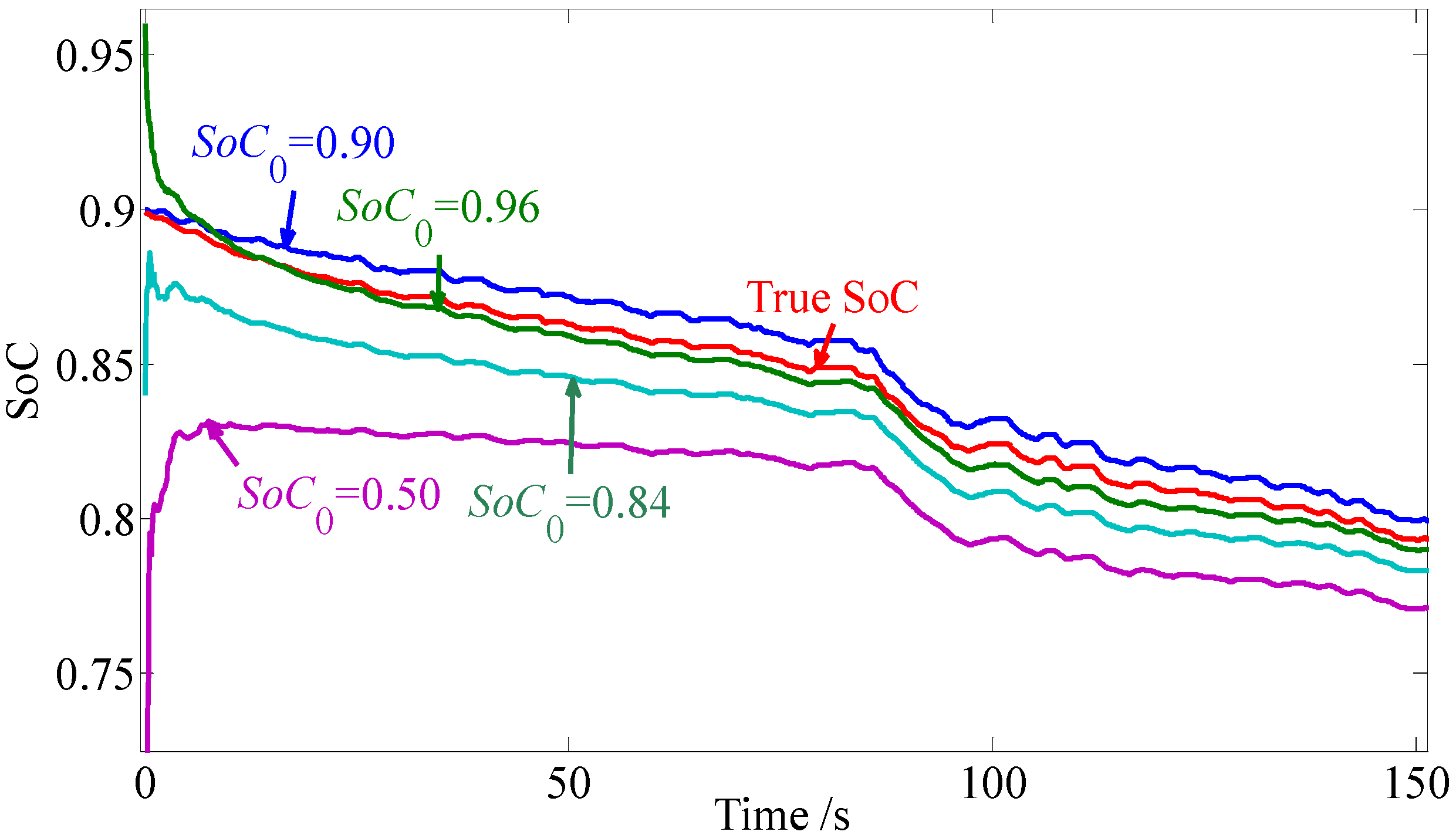
An accurate SoC estimation depends on two aspects according the definition of SoC given by Equation (15), one is the initial SoC, and the other is the calculation of SoC consumption. From the comparison in Section 4.3.1, the DP model has the highest accuracy for the SoC estimation under the assumption of a precise initial SoC value. In order to investigate whether the SoC estimation with REKF algorithm and the DP model, can effectively solve the initial estimation inaccuracy of SoC, a further simulation analysis is conducted. Four different SoC initial values, 0.90, 0.96, 0.84 and 0.50, are preset and the corresponding SoC estimations are performed based on the FUDS cycles, at the same time, a true SoC is calculated with the true initial SoC of 0.899 based on the FUDS test data. The results are shown in Figure 15 for the first 150 s and the results of the statistic analysis on the absolute SoC estimation error between the true value and the estimation during 151 s~15775 s are listed in Table 9. It can be seen that the estimated SoC can effectively converge around the true SoC within 150 s, no matter which initial SoC value is used and its terminal error is within 1.56%.

Figure 15. The SoC estimation profiles with different SoC initial values.

Figure 15. The SoC estimation profiles with different SoC initial values.

Table 9. The statistical list of absolute SoC estimation errors with different initial SoC values after 150 s and the terminal error.

SoC0	Maximum	Mean	Variance	Terminal Error
0.90	0.0098	0.0051	2.65 × 10−5	0.0070
0.96	0.0181	0.0080	1.79 × 10−5	0.0073
0.84	0.0279	0.0105	7.40 × 10−5	0.0103
0.50	0.0352	0.0144	3.68 × 10−4	0.0156

Table 9. The statistical list of absolute SoC estimation errors with different initial SoC values after 150 s and the terminal error.

SoC0	Maximum	Mean	Variance	Terminal Error
0.90	0.0098	0.0051	2.65 × 10−5	0.0070
0.96	0.0181	0.0080	1.79 × 10−5	0.0073
0.84	0.0279	0.0105	7.40 × 10−5	0.0103
0.50	0.0352	0.0144	3.68 × 10−4	0.0156

5. Conclusions

A dual polarization (DP) model is put forward based on the evaluations of the traditional models by adding an extra RC circuit to the Thevenin model simulating the electrochemical polarization and concentration polarization separately. Detailed evaluations on the Rint model, the RC model, the Thevenin model, the PNGV model and the DP model are carried out by experiments and simulations from the aspects of the dynamic performance and SoC estimation. It can be found that the proposed DP model has the best dynamic performance and gives a more accurate SoC estimation. In addition, the sensitivity of the different SoC initial values is examined based on the accuracy of the DP model-based SoC estimation with the REKF approach. It is clear that the error resulting from the SoC initial values is significantly reduced and the true SoC is convergent within an acceptable error.