1. Introduction
Interwell connectivity evaluation determines how effectively two wells are connected to each other. This can provide useful information on reservoir heterogeneity and lead to better waterflood management. Analysis of injection and production data can be particularly useful for determining connectivity between well pairs, since flow rates are among the most common measurements made during field life.
In the last two decades, several methods have been developed to analyze injection and production data and define parameters which evaluate the connectivity. Some of these connectivity parameters provide us with semi-quantitative insights to better understand the reservoir heterogeneity. For example, the correlation coefficient between injector-producer well pair flow rates [
1,
2] may help identify flow barriers or conduits between the well pairs. The correlation coefficient (
r), for example, could be used to rank well pairs for their connectivity. The use of
r, however, is not fully quantitative, because if one well pair has coefficient
r0 while another pair has 2
r0, the latter pair is not necessarily twice “as connected” as the former pair. Other, more fully quantitative parameters exist to assist us in waterflood management. For instance, the parameter
λ in the Albertoni and Lake Model [
3] and the Capacitance Model (CM) [
4,
5,
6] not only give a quantitative evaluation of the interwell heterogeneity but can be used to predict the waterflood performance. Such a connectivity parameter decouples the effect of injection rate from the flow data. Thus the connectivity parameter
λ will be independent of injection rate fluctuations. In cases where producer BHPs (bottom hole pressures) are available, the CM can also decouple the effect of pressure on
λ. There are, however, non-reservoir effects which still affect
λ, such as the well spacing and skin factors.
The CM is not the only tool recently proposed to analyze flow rates for interwell connectivity. Kaviani and Valkó [
7] developed the multiwell productivity index (MPI)-based method to evaluate interwell connectivity. The connectivity parameter obtained using the MPI method can decouple the effects of injection rate, producer BHPs, skin factor, and location of the wells from the apparent connectivity. Therefore, this connectivity parameter represents a quantity which is more nearly only a function of the heterogeneity between the well pairs. Since this method is independent of the number and condition of the wells, frequent shut-ins and stimulation treatments of producers have no effect on the performance of the method and can be used successfully for both heterogeneity evaluation and reservoir performance prediction. See Kaviani and Jensen [
8] for a comparison of the MPI and the CM methods for some synthetic cases.
The MPI method was originally developed for closed (volumetric) reservoirs, however. In non-volumetric (open) reservoirs, depending on the amount of fluid loss or gain, applying the MPI may lead to substantial errors in prediction of the production rates (with R2 < 0) or unrepresentative connectivity parameter values. The modifications described in this work show how we can analyze non-volumetric reservoirs to obtain improved predictions of reservoir performance (R2 > 0.99) and acceptable connectivity parameter estimates. Another problem with the MPI method is the relatively large number of model parameters for cases with medium to large numbers of wells (e.g., >25 wells). This will lead to a large CPU time needed for calculating the model parameters. We introduce windowing, a model reduction technique, to effectively reduce the number of parameters and so decrease the CPU time (for the studied cases up to 20 times) to evaluate reservoirs with large numbers of wells.
2. MPI Method
We begin with a brief review of the MPI method. For more details regarding the MPI concept, see [
9,
10].
In a reservoir with one well, under pseudosteady state conditions, we can calculate the production rate using:
where
q is the production rate,
J is the productivity index, and ∆
p is the pressure drawdown at the well location. Drawdown is defined as the difference of the well and volumetric average pressures. By defining the MPI, Valkó
et al. [
10] extended the productivity index concept to systems with multiple producing wells:
where
is the vector of total liquid (water and oil) production rates, [
J] is the multiwell productivity index matrix, and
is the vector of pressure drawdowns at the wellbore locations. [
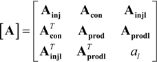
J] can be expressed in terms of the influence matrix, [
A]:
where
к is the rock-fluid factor, equal to 2π
kh/(
μB), where
k is the reservoir permeability,
h is the reservoir thickness,
μ is the liquid viscosity, and
B is the formation volume factor. [
A] can be calculated analytically for a rectangular homogeneous reservoir. The elements of this matrix are constant as long as the pseudosteady state assumptions are valid.
Kaviani and Valkó [
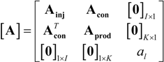
7] extended the MPI concept to systems having both injectors and producers. The influence matrix for a set of injectors and producers can be partitioned:
where
a is the influence function between the well pairs, the subscripts
inj indicates the injectors and
prod indicates the producers,
I is the number of injectors,
K is the number of producers, [
Ainj] is the influence matrix of the injectors, [
Acon] is the influence matrix between the injectors and producers, and [
Aprod] is the influence matrix of the producers. Based on this, the liquid production rate,
, will be:
Where
is the volumetric average reservoir pressure, [
1]
K×1 is a
K × 1 matrix with elements of 1,
is the vector of producer BHPs and
is the vector of injection rates [
7].
is a function of time and can be calculated as:
where
t is the time elapsed since the most recent change of state,
t =
t0 (here we define a new state after any change of the control parameters, including injection rate, producer BHPs and well skin factor),
is the volumetric average reservoir pressure at the previous state,
ct is the total compressibility,
Vp is the reservoir pore volume and
c1 and
c2 are defined as:
and:
We can also show that the injector BHPs,
will be:
The most important assumptions of this approach are that we have a volumetric (closed) reservoir and unit end-point mobility ratio of the phases [
9]. For a homogeneous and rectangular system, we can determine [
A] analytically. For such cases, we can easily calculate the reservoir performance at any time. For heterogeneous reservoirs, however, no analytical formula exists to determine [
A]. For these cases, we have to estimate [
A] based on the injection and production data: the matrix that minimizes the error in prediction of production rates and injector BHPs (if available) is the influence matrix for a heterogeneous system ([
A(H)]). In other words, we back-calculate the influence matrix based on reservoir performance. We can use a nonlinear numerical solver to estimate this matrix. Kaviani [
9] discusses the possible issues with non-uniqueness of this matrix under different situations. The difference between this matrix and the analytical influence matrix (from the homogeneous case with the same reservoir extent and well location) is called the
heterogeneity matrix ([
∆]):
The analytical influence matrix contains the well location, reservoir extents and well skin factor components of the apparent connectivity between the wells. The heterogeneity matrix solely represents the heterogeneity-related components of the interwell connectivities. Similar to the influence function, this matrix is symmetric. Each off-diagonal element of this matrix (
δ) is called the
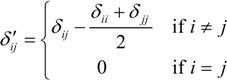
connectivity index between the corresponding wells defined by the row and the column of the heterogeneity matrix. By modifying the connectivity indices using:
a more robust indicator of connectivity will be obtained that is called the
modified connectivity index [
7]. In general,
δ´ij > 0 when there is a large connectivity in the interwell (and vicinity) region and
δ´ij < 0 indicates a small connectivity between the wells [
7]. Thus,
δ´ij = 0 represents an intermediate level of connectivity between wells, such as we would have for a completely homogeneous reservoir; it does not represent zero connectivity.
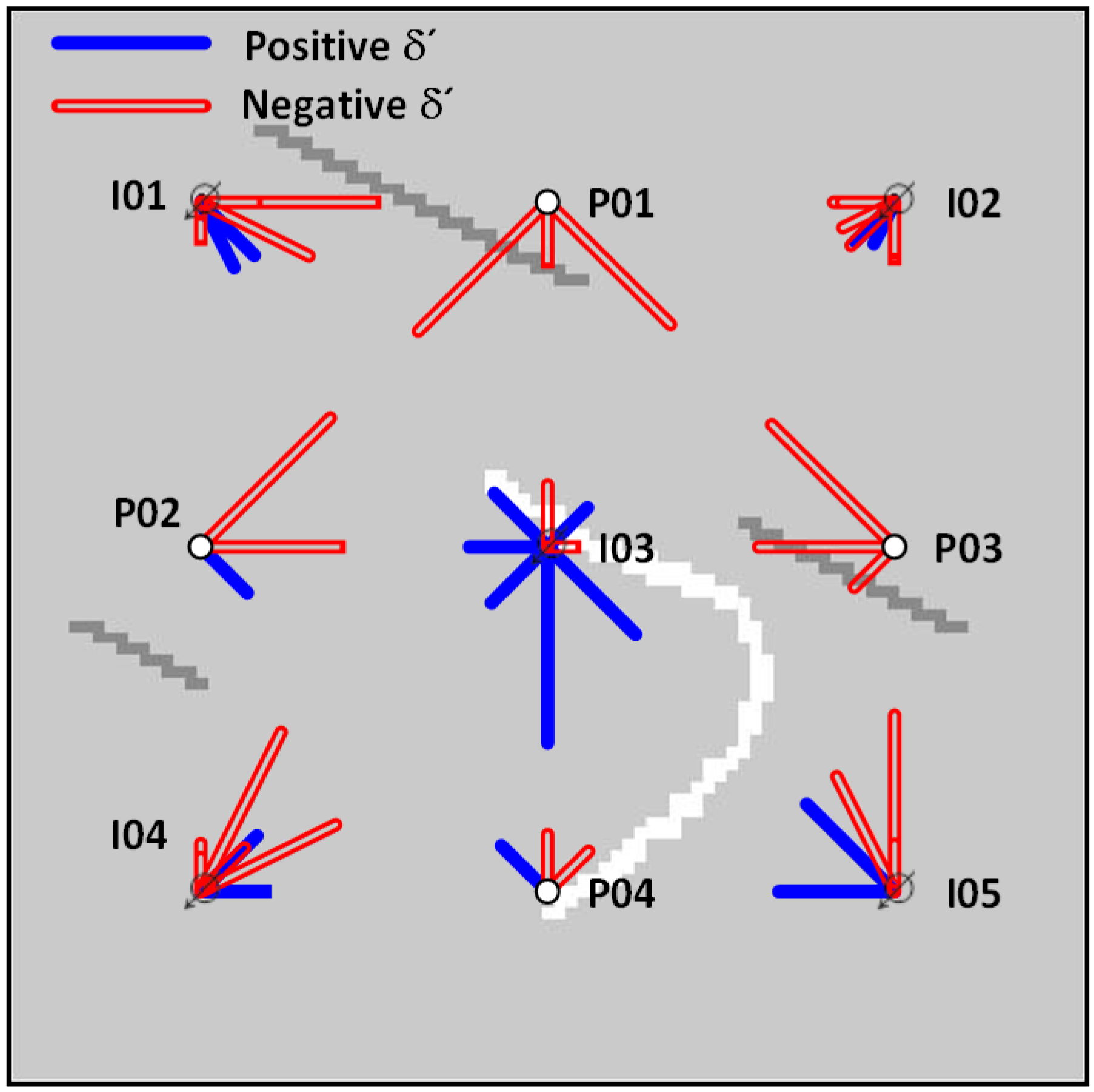
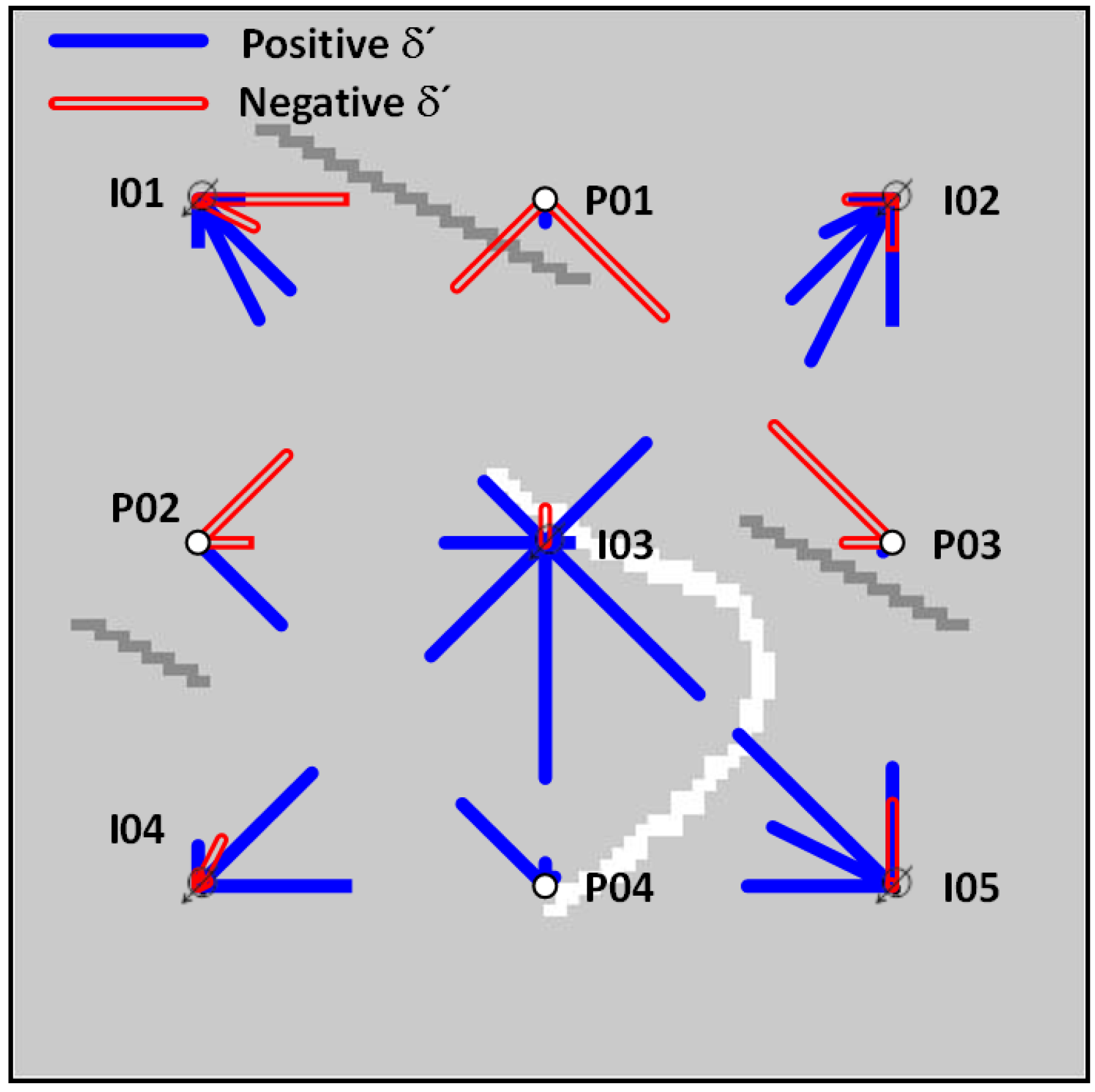
We can use a simple vector map (very similar to the maps of Albertoni and Lake [
3]) to show the connectivity of the system. In this map, we draw a vector from each injector to the other injectors and producers where the vector length shows the absolute magnitude of the modified connectivity indices (
δ´ij). To show the connectivity between producers, we draw the vectors from both wells. The light (red) vectors show the
δ´ij < 0 and heavy (blue) ones represent
δ´ij > 0. For example, for a heterogeneous reservoir (
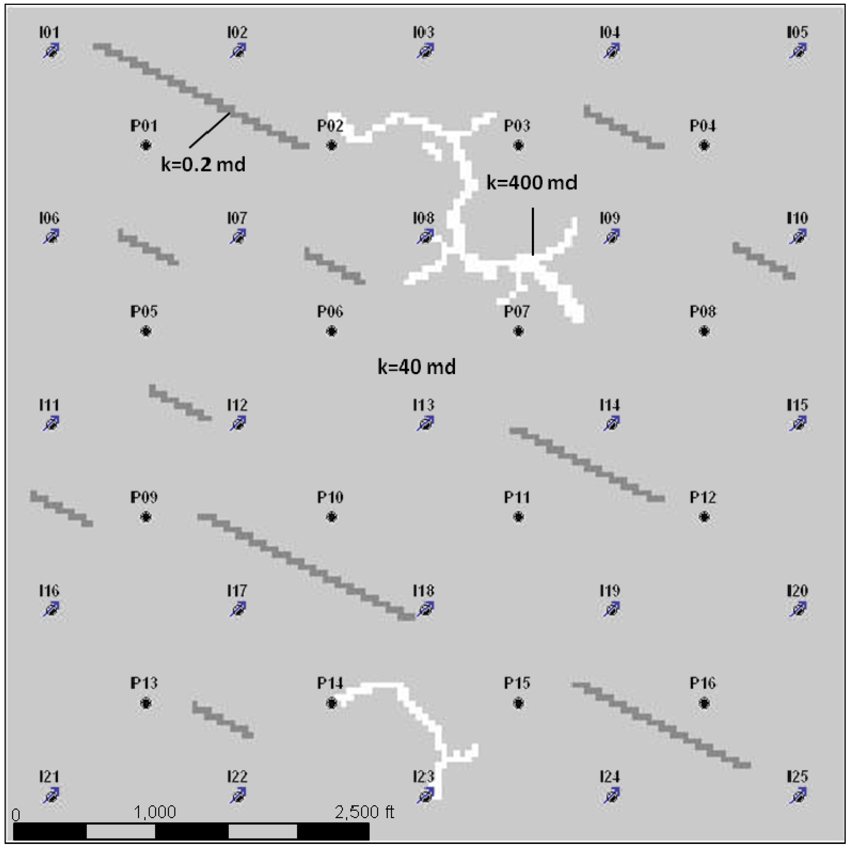
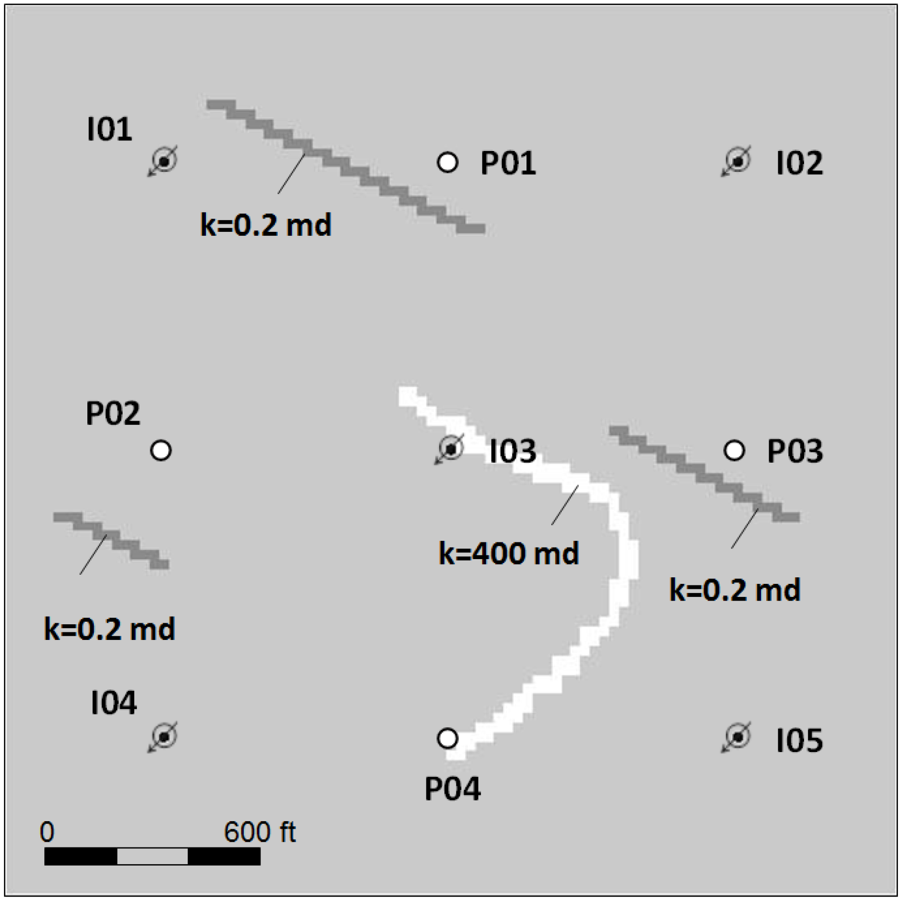
Figure 1 with properties listed in
Table 1), the connectivity map (
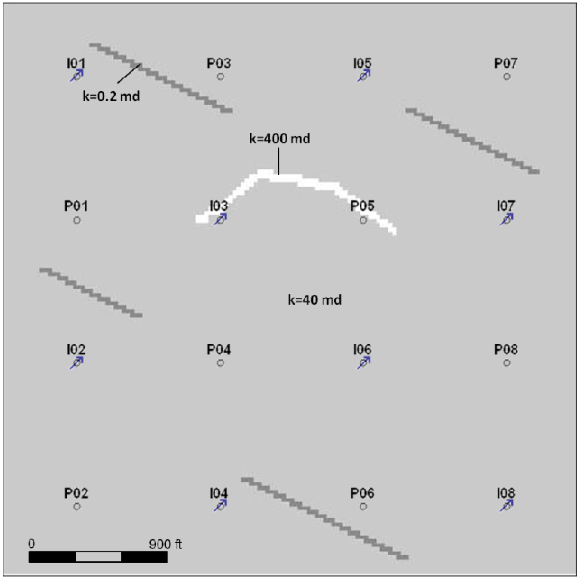
Figure 2) shows the main geological features clearly.
δ´(I03, P04) > 0 and
δ´(I03, I05) > 0, reflecting the channel in their interwell regions.
δ´(I01, P01) < 0,
δ´(P01, P02) < 0, and
δ´(I05, P03) < 0, reflecting the barriers near these well pairs. (For more discussion of the interpretation of this map, see [
7].)
Figure 1.
Permeability map and well locations of Case 1. The permeability of the reservoir is 40 md and there are three barriers with permeability of 0.2 md and a channel with permeability of 400 md.
Figure 1.
Permeability map and well locations of Case 1. The permeability of the reservoir is 40 md and there are three barriers with permeability of 0.2 md and a channel with permeability of 400 md.
The procedure to determine the modified connectivity indices can be summarized as:
Calculate the analytical influence function of the wells based on well locations and reservoir extents.
Evaluate the optimum influence matrix that minimizes the reservoir performance (production rates and injectors’ BHP) prediction error.
Calculate the heterogeneity matrix and modified connectivity indices.
We term this the “simple MPI” method because it assumes a closed system and uses data from all wells in the system.
Table 1.
General Fluid and rock properties of the simulated cases.
Table 1.
General Fluid and rock properties of the simulated cases.
| Reservoir Thickness | h = 60 | ft |
| Porosity | φ = 0.18 | |
| Permeability | Absolute = 40 | md |
| Oil end point = 36 | md |
| Water end point = 9 | md |
| Viscosity | Oil = 0.5 | cp |
| Water = 2 | cp |
| Formation Volume Factor | Oil = 1.07 | |
| Water = 1.01 | |
| Compressibility | Oil = 5 × 10⁻⁶ | psi−1 |
| Water = 1 × 10⁻⁶ | psi−1 |
| Rock = 1 × 10⁻⁶ | psi−1 |
Figure 2.
In connectivity maps, the length of the vector between each well pair shows the connectivity level (δ´ij). For the injector/producer well pairs, we draw a vector only from the injectors. For the injector well pairs and the producer well pairs, we draw vectors from both wells. In this example, large (heavy blue line) δ´(I03, P04) and δ´(I03, I05) indicate the channel in their interwell region. Small (light red line) δ´(I01, P01), δ´(P01, P02), and δ´(I05, P03) are indication of barriers between these wells.
3. Non-Volumetric Systems
One of the main assumptions in the MPI approach is that the reservoir is a closed system. In other words, we assume all the fluid injected will be stored or eventually produced and there is no additional source of energy (e.g., aquifer) or leaking elements (e.g., leaking fault) that affects production rates. We also assume that all the injectors and producers in the system are included in the analysis. In such cases, we expect the total injection rate to be similar to the total production rate. Thus, if we observe a large difference between these two or we are aware of a leaking zone or an aquifer in the system, the volumetric assumption is not valid. Since these situations are common in fields, we develop some modifications to mitigate these effects on the MPI.
Ideally, if we know the location and properties of the leak zones, we may model them by adding wells at the location of the leak zones. However, such information is most likely unavailable. To model this effect, we assume all the leaked fluid is produced from a virtual well (with constant BHP) in the system. To include this well in the model we need to modify the influence matrix of the system (Equation 4). In this approach the influence function can be written as:
where [
Ainjl] is the
I × 1 matrix of the influence functions between the injectors and virtual well, [
Aprodl] is the
K × 1 matrix of the influence functions between the producers and virtual well, and
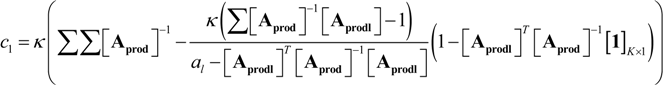
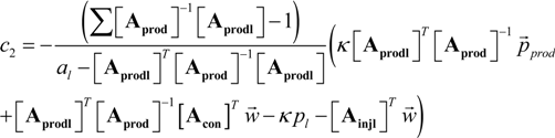
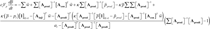
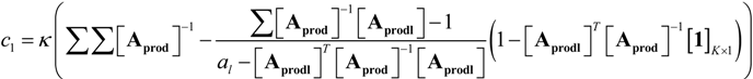
al is the influence function of the virtual well. We can show that the average reservoir pressure of the system for this case will be in the form of Equation 6, where
c1 and
c2 are (
Appendix A):
where
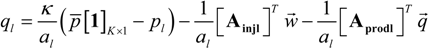
pl is the BHP of the virtual well. The vector of liquid production rates will be:
where
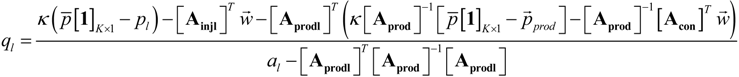
ql is the production rate of the virtual well and can be calculated as:
In this case, the injector BHPs will be:
If injection and production data are available, we can determine the
I +
K + 2 new parameters ([
Ainjl], [
Aprodl],
al, and
pl) using the same procedure as used to calculate the heterogeneity matrix. To reduce the number of parameters of this model, we can use a reduced form of the influence matrix of Equation 12. By assigning zero to the off-diagonal elements of the virtual well row and column of the influence matrix, we obtain:
where [
0]
I×1 is a
I × 1 matrix with elements of 0. The “zero” elements of the influence function between the virtual well and other wells does not mean the absence of connectivity between these wells (
Appendix A). For this reduced approach, the average reservoir pressure is calculated using Equation 6 with:
and
and Equations 5 and 9 still apply for calculating
and
g the reduced approach, we only need to add two new parameters to the model:
al, and
pl. Instead of the zero-vector, we may have any other constant matrix and it does not affect the model performance; however, the advantage of the zero-vector is its simple solution where several terms in the equations cancel. In this paper, we call the approach with the full influence matrix with a virtual well the “full leak model” (Equation 12) and the one with reduced matrix (zero elements for the virtual well) the “reduced leak model” (Equation 18).
We now apply the developed approaches for three synthetic systems, where we used a commercial simulator (Eclipse 100™) to calculate the reservoir performance. For all cases, we first determined the δ´ for a similar ideal case, where all model assumptions are met, e.g., closed boundary system and unit end-point mobility ratio, and with the same well locations and geological properties. Then we compared the estimated δ´ for the open reservoirs with these “true” values.
Case 1. This case is a 5 × 4 heterogeneous system (five injectors and four producers,
Figure 1). The rock and reservoir properties are listed in
Table 1. At first we simulated a reference case with a closed system and, based on the simulated injection and production data, we evaluated the modified connectivity indices of the system (
Figure 2 and
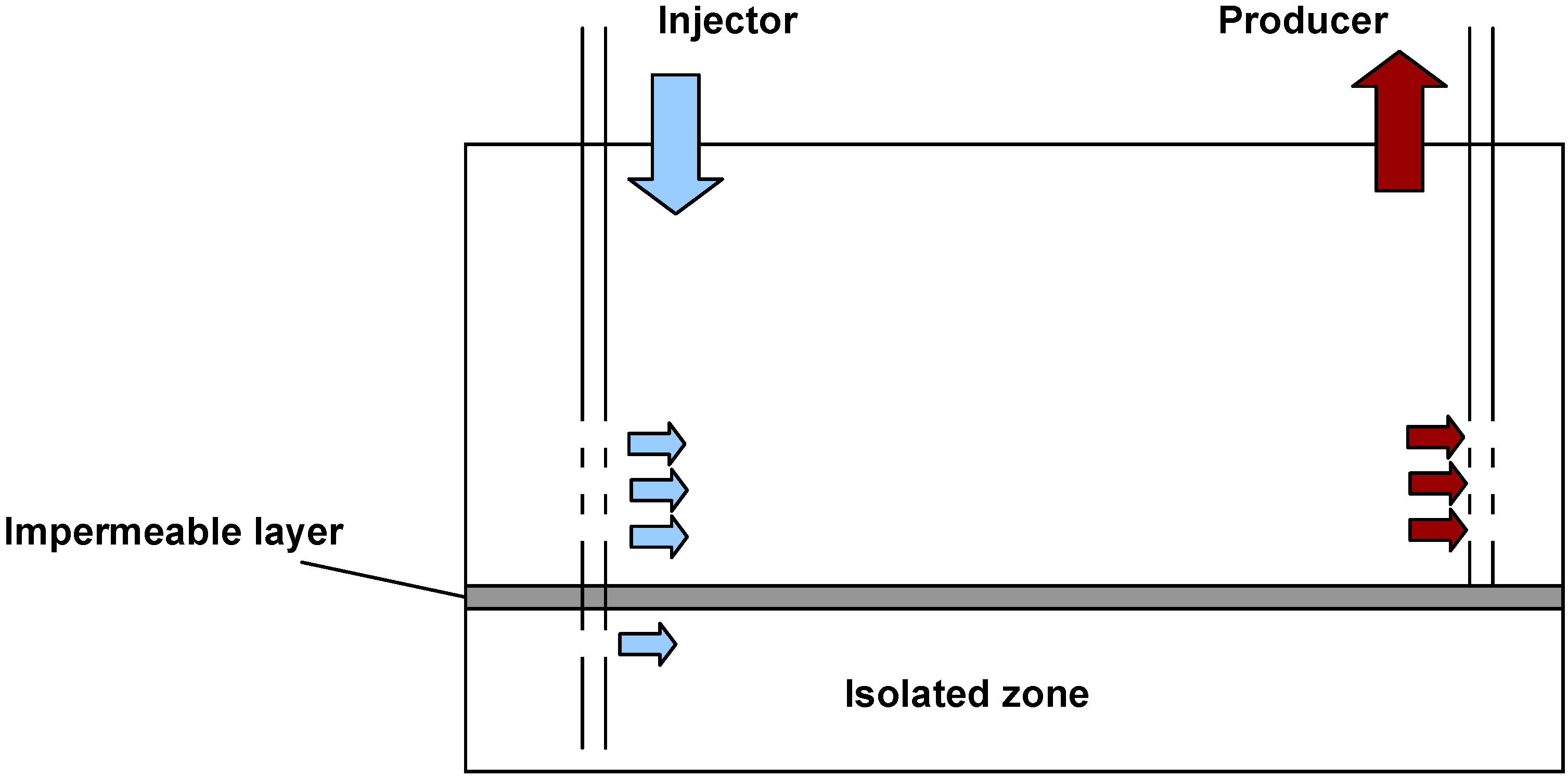
Table 2). Then we added an “isolated” zone to the system that is not connected to the reservoir (
Figure 3). In this case, more than 3% of the injected fluid was lost to the isolated zone. Applying the full leak and reduced leak models, we observed the leak models could predict the reservoir performance much more accurately than the simple model (
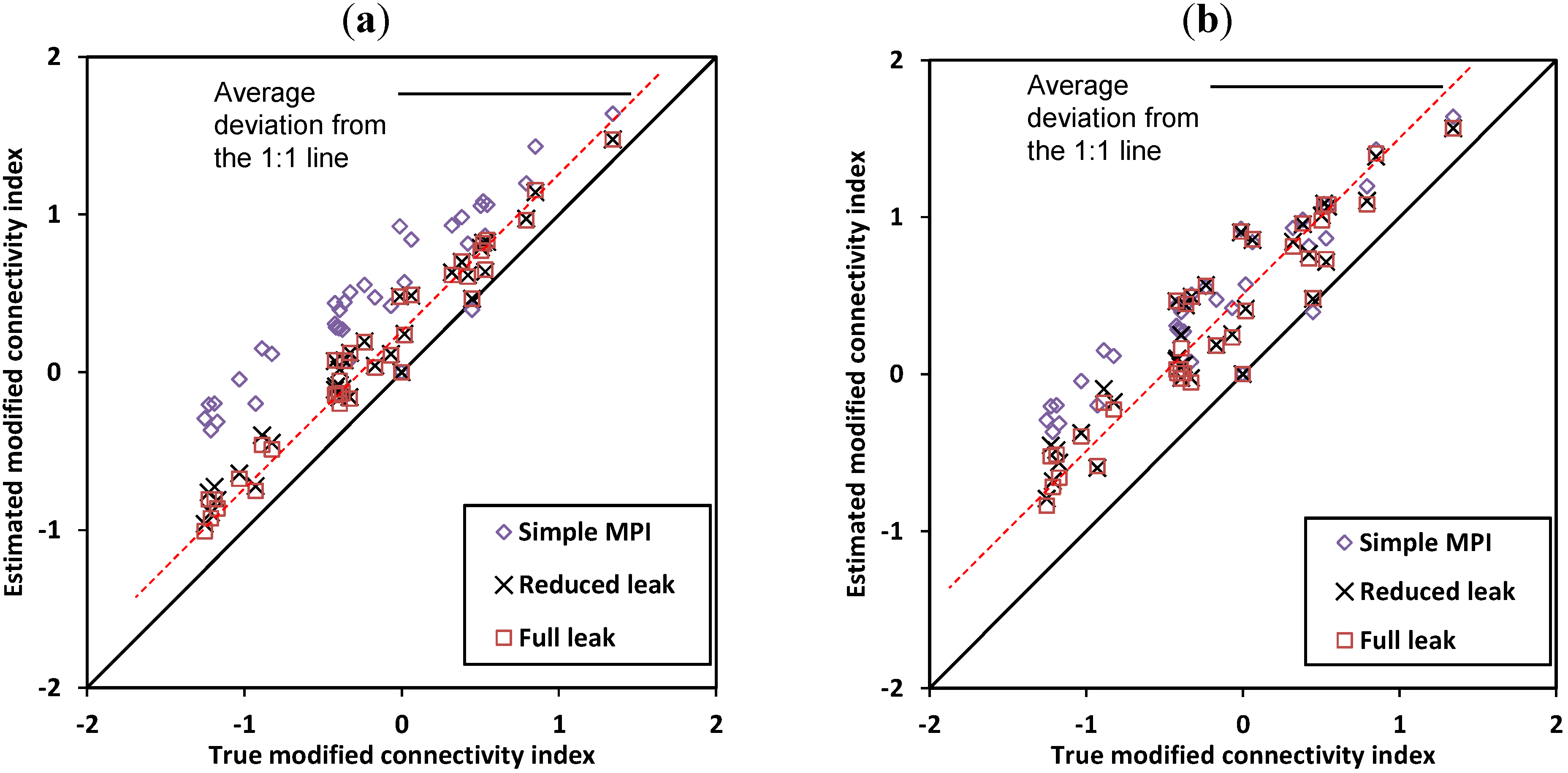
Table 2). On the other hand, comparing the estimated
δ´ with the true
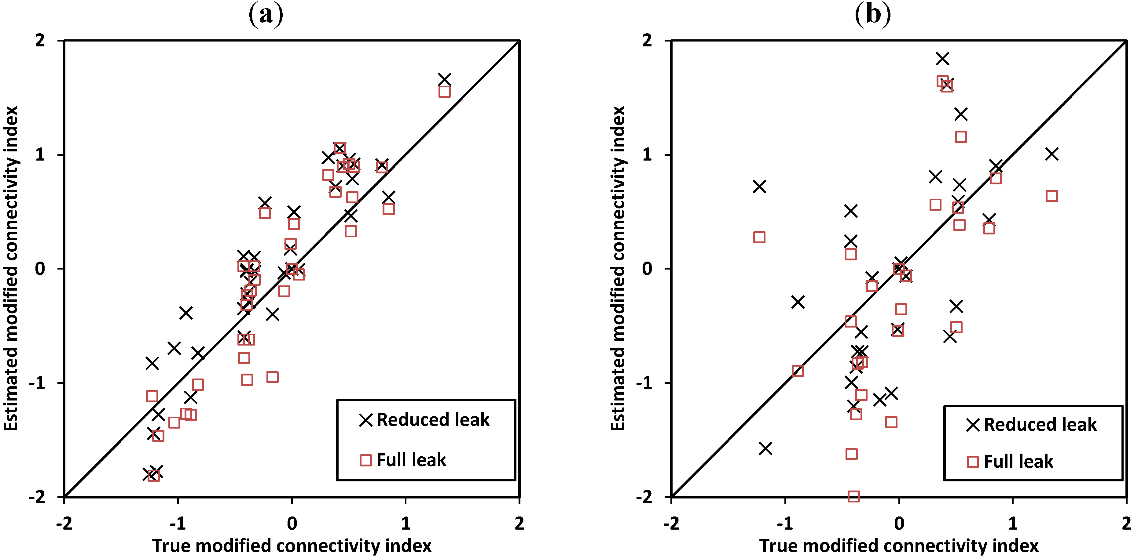
δ´, the difference is only 0.26 in average (
Figure 4a). We also tested a case with a larger isolated zone where almost 6% of the injected fluid escaped to the isolated zone. Applying all three models, the performance of the simple model decreased markedly, especially for the predicted
vs. production rates (
R2 = 0.67). The full and reduced leak models provide accurate estimation of reservoir performance; however, the estimated
δ´ were less accurate (on average 0.46 difference in estimated
δ´) than for the 3% leakage case (
Figure 4b).
Table 2.
Comparison of reference and non-ideal model results using R2.
Table 2.
Comparison of reference and non-ideal model results using R2.
| | Model | Production Rate | Injectors’ BHP |
|---|
| Case 1, closed system | Simple model | 1.000 | 1.000 |
| Case 1, small isolated zone | Simple Model | 0.906 | 0.999 |
| Full leak model | 0.999 | 1.000 |
| Reduced leak model | 0.999 | 1.000 |
| Case 1, large isolated zone | Simple Model | 0.669 | 0.997 |
| Full leak model | 0.999 | 0.999 |
| Reduced leak model | 0.998 | 0.999 |
| Case 2 | Simple Model | −11.849 * | 0.991 |
| Full leak model | 1.000 | 1.000 |
| Reduced leak model | 1.000 | 1.000 |
| Case 3 | Simple Model | −26.642 * | 0.967 |
| Full leak model | 1.000 | 1.000 |
| Reduced leak model | 1.000 | 1.000 |
| Case 3, with 20% noise | Simple Model | −21.230 * | 0.796 |
| Full leak model | 0.754 | 0.807 |
| Reduced leak model | 0.756 | 0.806 |
| Case 3, with 40% noise | Simple Model | −11.154 * | 0.487 |
| Full leak model | 0.427 | 0.491 |
| Reduced leak model | 0.427 | 0.490 |
Figure 3.
Case 1 configuration where every injection well has fluid loss to the isolated zone.
Figure 3.
Case 1 configuration where every injection well has fluid loss to the isolated zone.
Figure 4.
For the (a) small (3%) and (b) large (6%) isolated zone cases, the approaches generate modified connectivity indices that are slightly higher than the true ones. The results of the full and reduced leak models are almost identical.
Figure 4.
For the (a) small (3%) and (b) large (6%) isolated zone cases, the approaches generate modified connectivity indices that are slightly higher than the true ones. The results of the full and reduced leak models are almost identical.
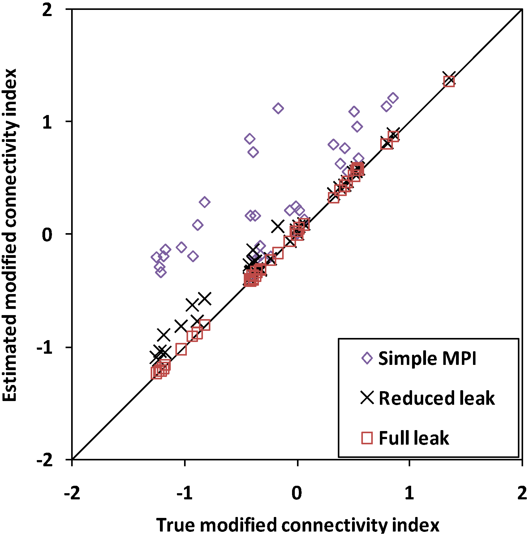
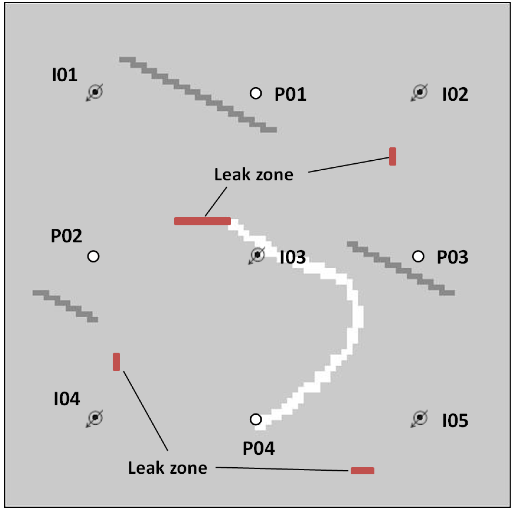
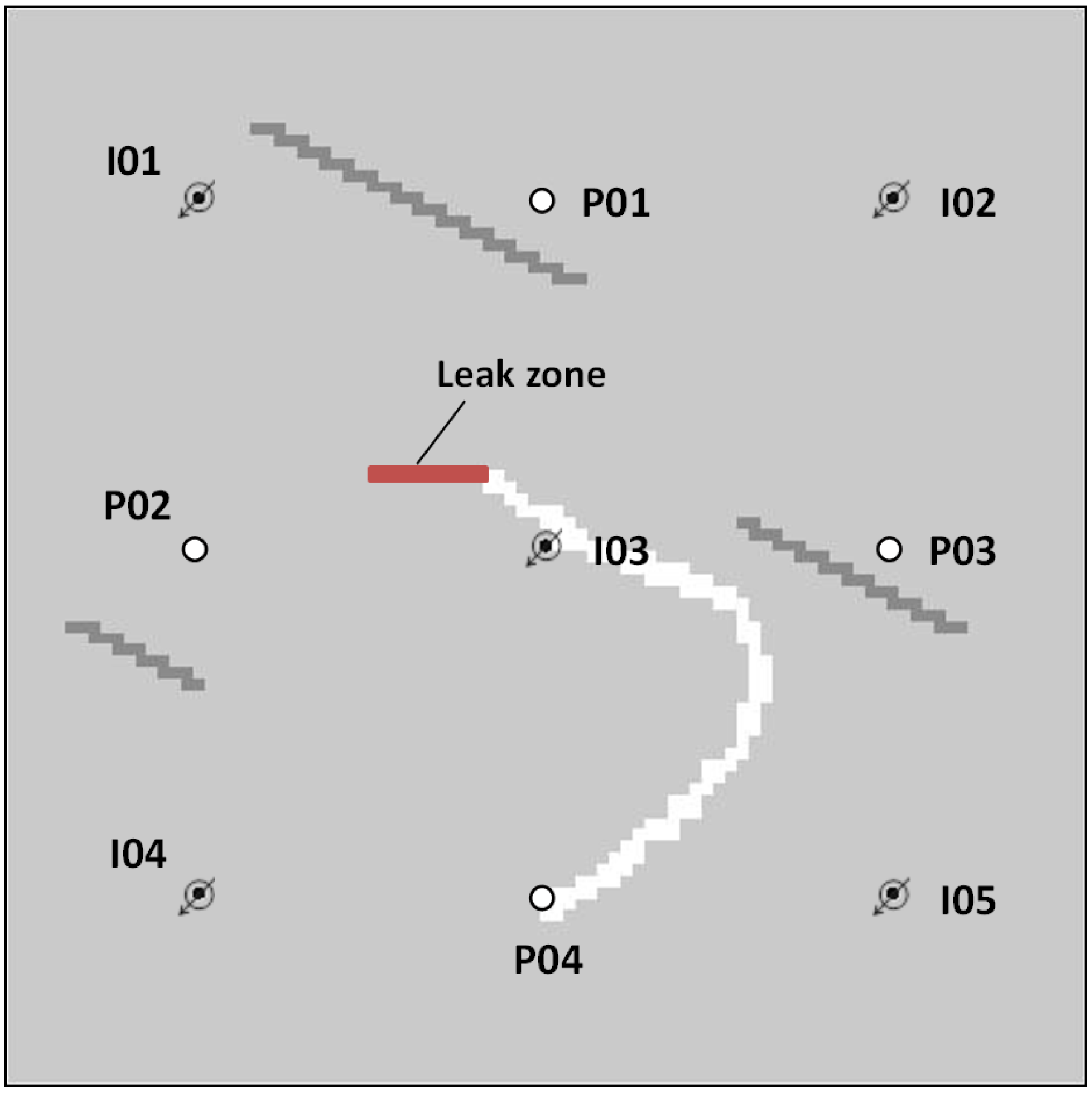
Case 2. The well locations, geometry and the heterogeneity of the reservoir are similar to Case 1. However, for this case we have a localized leaky zone (
Figure 5) where almost 27% of the injected fluid is escaping. Applying both full and reduced models, we can accurately model the data (
Table 2). The simple MPI gives very poor results. On the other hand, the full model predicted the
δ´ more accurately than the other models (
Figure 6). Since we only have a localized leak in this case, the full model also determined the parameters of that leak zone as an additional well and reproduced the exact
δ´s.
Figure 5.
In Case 2, a leak zone exists in the system, where 27% of the injected fluid leaks out from the system.
Figure 5.
In Case 2, a leak zone exists in the system, where 27% of the injected fluid leaks out from the system.
Figure 6.
For Case 2, the full leak model estimates the δ´ more accurately than the other methods. The prediction of the reduced model is also excellent.
Figure 6.
For Case 2, the full leak model estimates the δ´ more accurately than the other methods. The prediction of the reduced model is also excellent.
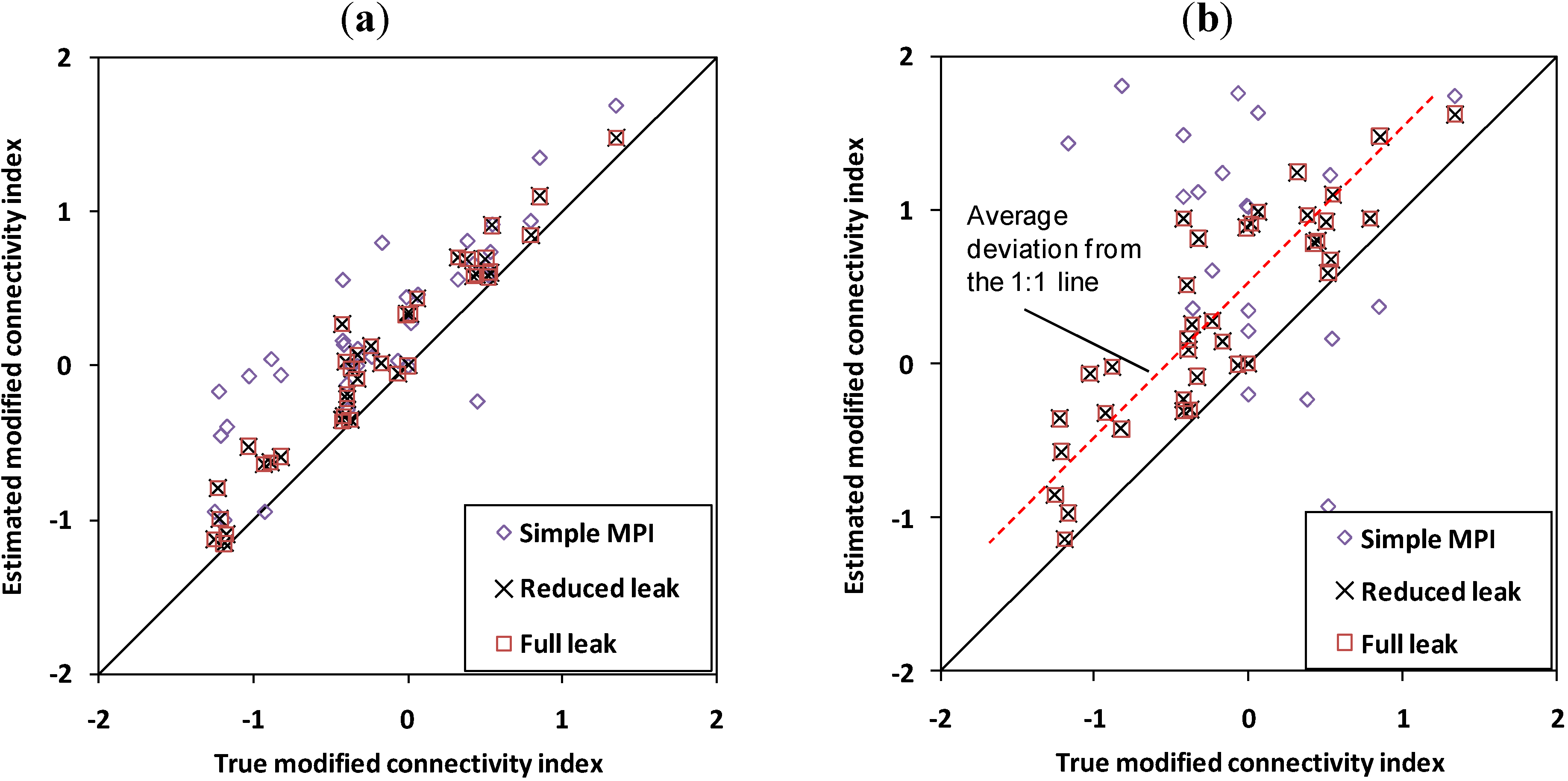
Case 3. This case is similar to Case 2, but the leaks are more widely distributed in the system (
Figure 7), where almost 35% of the injected fluid is leaking out from the system. A major fraction of the escaping fluid (more than two-thirds) is from one of the leaks. Similar to Case 2, both the full and reduced approaches fit the data very well (
Table 2). The estimated
δ´s from both reduced and leak model are almost identical and fairly close to the true ones (
Figure 8a). We also tested this case with the leak evenly distributed between the leak zones and a total of 47% escaping. For this situation, both the reduced and leak model predicted the reservoir performance perfectly. The estimated modified connectivity indices are, however, different from the true ones (
Figure 8b). Mapping these indices still shows useful connectivity information (
Figure 9). For instance, the channel around I03, and the barriers between (P01, P02) and (P03, I03), and (I01, P01) are recognizable. However, a few connectivity indices are misleading, e.g., (I02, I05) where no high permeability zone exists in the interwell region.
Figure 7.
For Case 3, four leak zones are in the reservoir, where 47% of the injected fluid is leaking from the system.
Figure 7.
For Case 3, four leak zones are in the reservoir, where 47% of the injected fluid is leaking from the system.
Figure 8.
For Case 3, where the major leak is from one location both reduced and full leak models provide good estimates of the modified connectivity indices (a). For the case with uniform leakage from the four locations none of the models predicts the modified connectivity indices accurately (b). The leak models, however, estimate the δ´ more accurately than the simple MPI.
Figure 9.
Connectivity map of Case 3 (with multiple uniform leaks) has useful information on the main barriers and channel in the system.
Figure 9.
Connectivity map of Case 3 (with multiple uniform leaks) has useful information on the main barriers and channel in the system.
To investigate the effect of noise on the results, we reran Case 3 (with 35% overall escape and one leak consuming 20%) while the response data were corrupted with different levels of uniformly distributed white noise. We observed that for 20% noise in the data, compared to the noise-free cases, the standard deviation of the
δ´ values is around 0.23, which shows a moderately accurate estimation (
Figure 10), and the predicted reservoir performance is acceptable (
Table 2). However, at 40% noise we cannot get any useful information from the data; the
R2 of predicted production rates and injectors’ BHP is smaller than 0.5 and the standard deviation of
δ´ values is larger than 1.
Figure 10.
For small amounts of noise (20%) the δ´ values are fairly accurate (a). Larger noise (40%) levels may lead to unrepresentative δ´ (b).
Figure 10.
For small amounts of noise (20%) the δ´ values are fairly accurate (a). Larger noise (40%) levels may lead to unrepresentative δ´ (b).
For all three cases, the production prediction accuracies of both the full and reduced approaches were very similar to each other and both methods are as accurate as or better than the simple model. The
δ´ predictions suffered when leakage was present and the estimated
δ´ values tended to overestimate the non-leak values by approximately 0.5 (
Figure 8b). For all the cases, the accuracy of the estimated
δ´ values and predicted reservoir performance for both full and reduced leak models were very close to each other; using the full model did not improve the results. Since in general, we may have more than one leak zone in the system, using the reduced model instead of the full model could be better because having fewer free parameters decreases the chance of overfitting the model to the data. On the other hand, considering the reduced accuracy of the estimated parameters for the case of multiple leaks (with similar sized leaks from different leaking points), one may consider using more than one virtual well. For example, if we use four vertical wells in Case 3 with 47% distributed leakage, the error becomes quite small. If the number of leaks is limited and we know the exact number of leaks this can increase the accuracy of the method. However, in general we do not know the number of leaks and adding more than one virtual well could lead to overfitting the model.
We have described MPI models which have been modified for mechanisms that lead to non-volumetric systems, and the leak models showed more accurate production predictions over the simple model. However, we have not yet devised a model which will produce accurate connectivity indices under all conditions. In practice, the leak mechanism might be different and more complicated than we have modeled here. For future work, considering more cases and mechanisms will help us to recognize the possible trends in the estimated connectivity indices (for example here, they were higher than the true ones) and interpret the results more accurately.
4. Large Number of Wells
In general, considering the symmetry of the heterogeneity matrix, we need to determine at least (
I +
K) × (
I +
K + 1)/2 parameters to model the system. For a small number of wells, evaluating these parameters can be done quickly. For larger numbers of wells, this procedure will be very time consuming and may become computationally intractable. For example, the CPU time required to model a 25 × 16 system may be three orders of magnitude longer than the time needed for an 8 × 8 case and four orders of magnitude longer than a 5 × 4 case. A possible strategy to overcome this problem is to eliminate the less important parameters that have only a small effect on reservoir performance predictions. Here, we describe a model reduction approach called
windowing. (Our use of the term windowing is similar to that used in signal processing and data analysis, e.g., [
13,
14].)
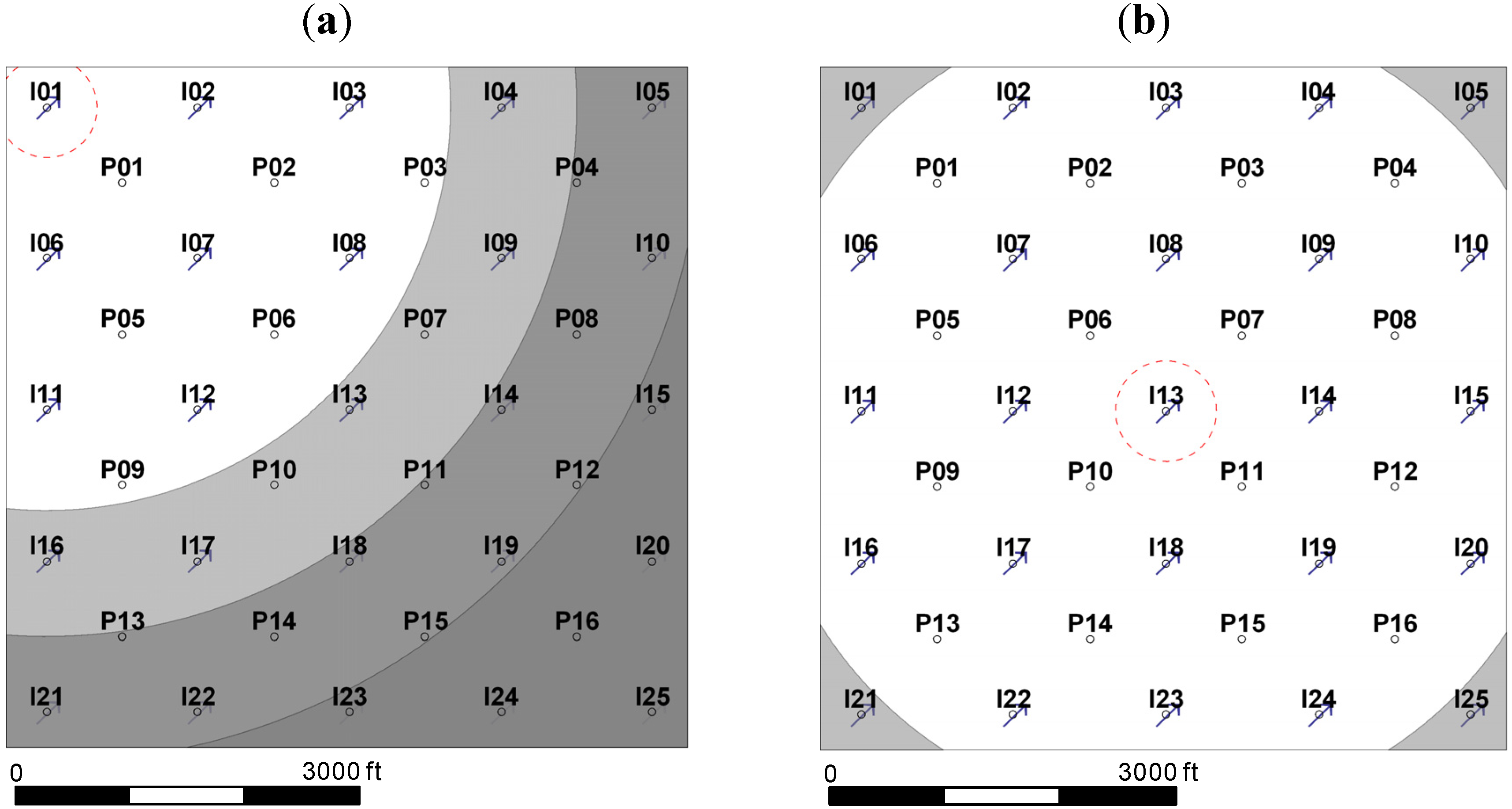
We define a region (window) for each well. This window can be defined based on distance of the wells and geology of the reservoir (if available). We only evaluate the connectivity indices between this well and the wells inside the window. For all the wells outside this window, we may calculate a single connectivity index (
Figure 11). If the number of wells is large, we may define several windows for each well, where at each region between windows, a single connectivity index is assigned to the wells (
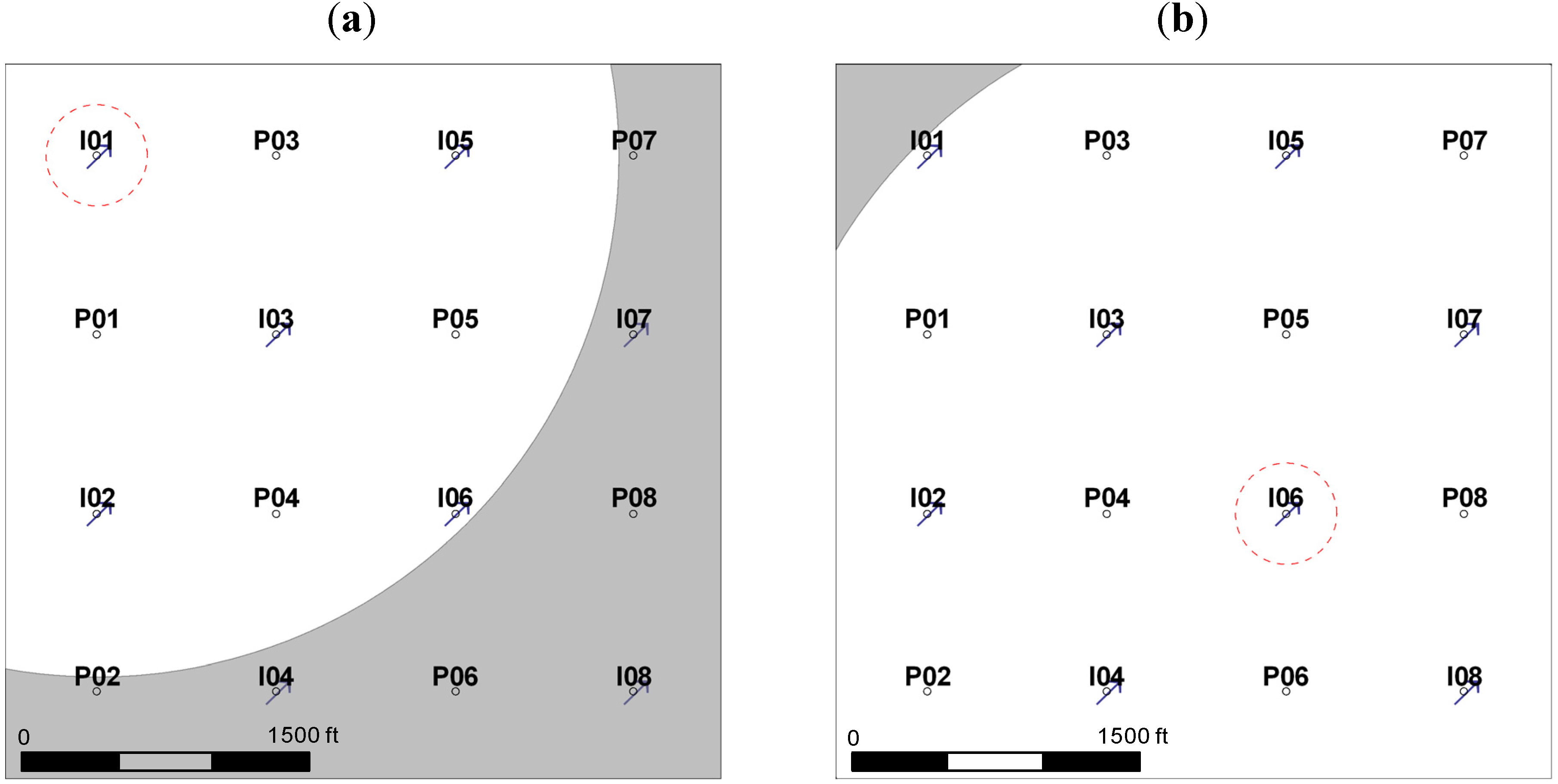
Figure 12). Depending on the number of wells and sizes of the windows, this technique can reduce the number of parameters dramatically. For example, for a 8 × 8 case (
Figure 11) with a 2750 ft window, the number of parameters decreases from 136 to 88 and for a 25 × 16 case (
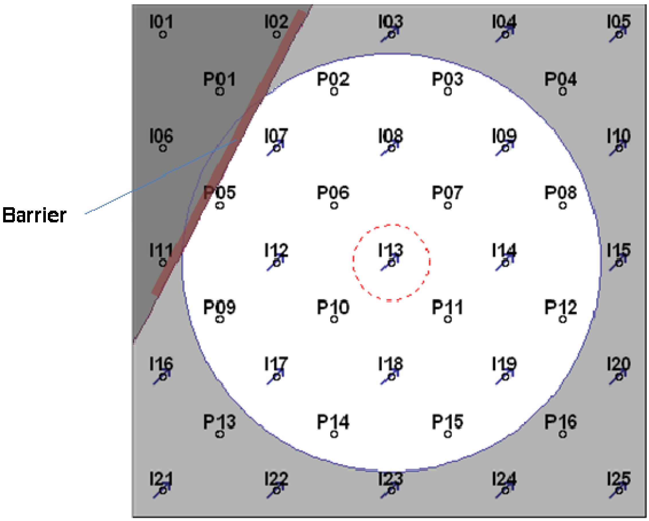
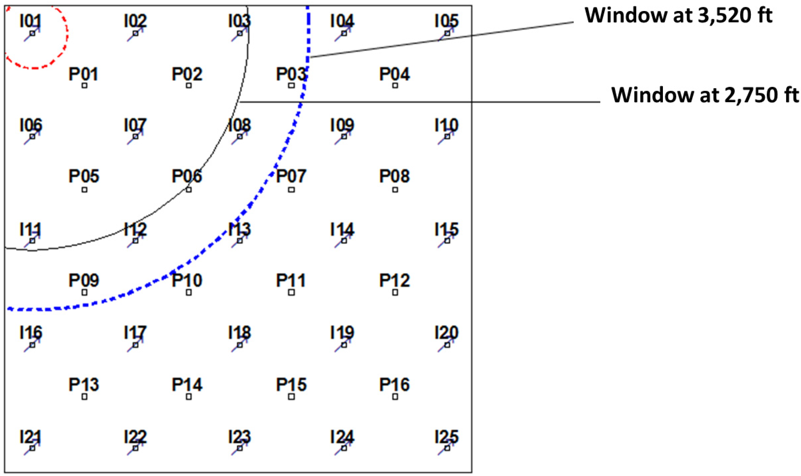
Figure 12), defining three windows at 3520, 4620 and 5720 ft, reduces the number of parameters from 861 to 425. In case we have some geological information about the reservoir, we may modify the shape of the window. For example, if we know a barrier exists in the reservoir, we can trim the window and add a new one to consider geological information in our model more effectively (
Figure 13). In systems with ovate or linear deposits, such as may occur in barrier bar or channel sediments, we may define elliptical widows to use the directional connectivity information in the model.
Figure 11.
In the windowing technique, we only estimate the connectivity indices between the target well and the wells inside the window. For wells outside the window, we assign a single value to all connectivity indices. In this 8 × 8 system, for well I01 (a), wells I04, I07, I08, P02, P07, P06, and P08 are outside the window. However, for well I06 (b), no well is outside the window.
Figure 12.
We can define more than one window for each well, where at each outer window a single value is assigned to the connectivity indices between the target well and the wells inside the window. Here, for well I01 (a), 7, 13 and 6 wells are in windows 1, 2 and 3, respectively. For well I013 (b), only four wells are outside the first window.
Figure 13.
If we have geological information about the field, such as the location of a flow barrier, we may change the window shape. Because of the barrier, we assigned a different window size for the wells to the left of the barrier.
Figure 13.
If we have geological information about the field, such as the location of a flow barrier, we may change the window shape. Because of the barrier, we assigned a different window size for the wells to the left of the barrier.
Here, we show two cases of windowing using numerical simulation.
Case 4. For this 8 × 8 heterogeneous system (
Figure 14), the fluid and rock properties are identical to Case 1. Based on the simulated injection and production data, we calculated the
δ´s of the system. We then defined a window at 2750 ft (
Figure 11) and modeled the data and the modified connectivity indices, which were in very good agreement with those from the model with no window (
Figure 15). The estimated
δ´s of the closer wells are slightly more accurate than the distant ones. In addition, the R
2 of the predicted production rates and the injectors’ BHPs were 0.9996 and 0.9998, respectively, showing that the model with the smaller number of parameters was adequate to predict the reservoir performance. Applying this window reduced the CPU time by more than 3.5 times.
Figure 14.
Permeability map of Case 4. Four barriers and one channel exist in the system. The well spacing is 945 ft.
Figure 14.
Permeability map of Case 4. Four barriers and one channel exist in the system. The well spacing is 945 ft.
Figure 15.
For Case 4, applying a window (as we have in
Figure 11) the estimated connectivity indices are in excellent agreement with the ones obtained using no window. The
δ´s of the closer well pairs (<1375 ft) are estimated slightly more accurately than the more distant ones (between 1375 ft and 2750 ft).
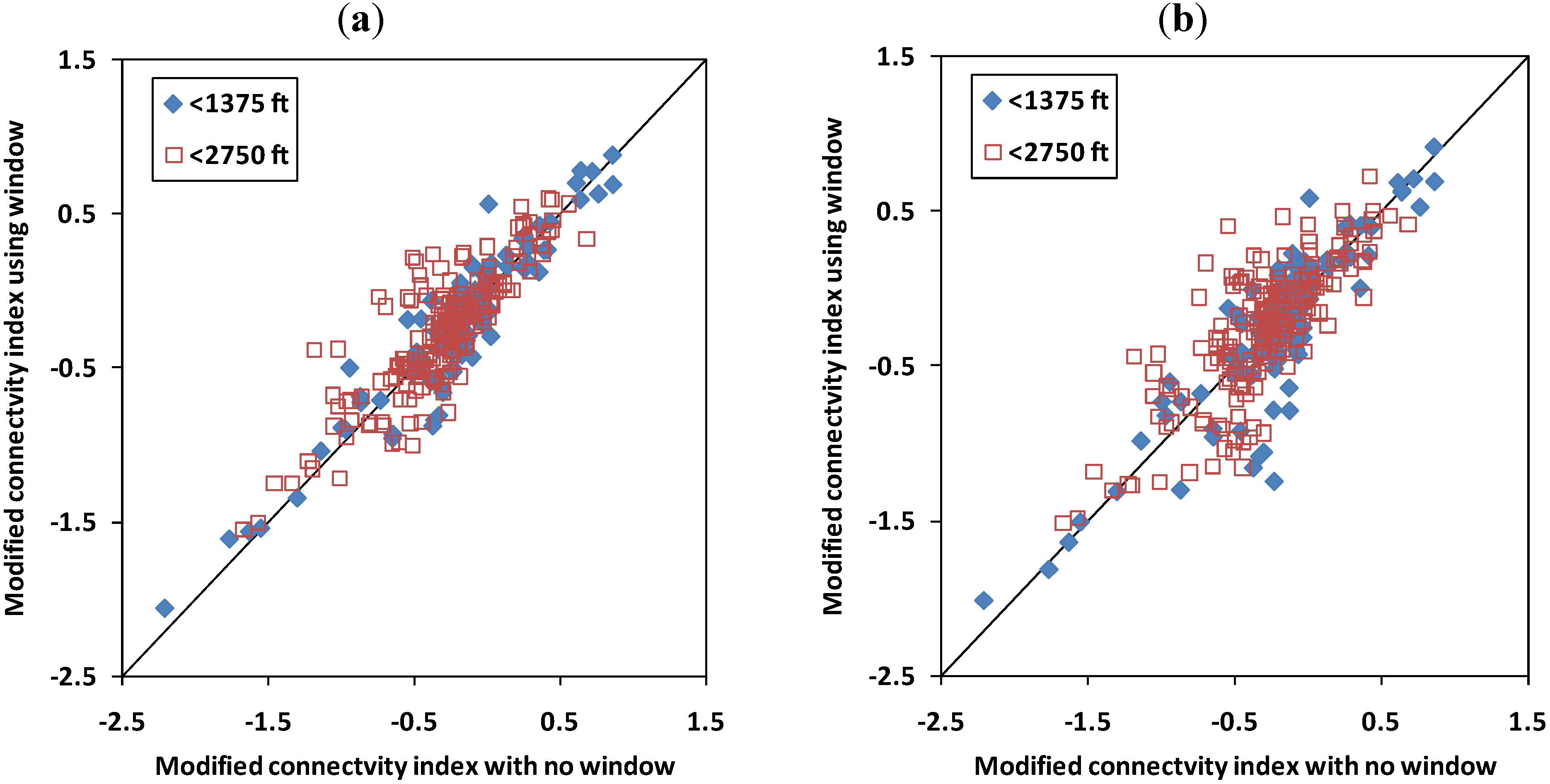
Case 5. This case is a 25 × 16 heterogeneous reservoir (
Figure 16) with rock and fluid properties identical to Case 1. At first, we applied a window at 2750 ft (
Figure 17) that reduced the number of free parameters from 861 to 254. The
R2 values of the predicted production rates and injectors’ BHPs were 0.9926 and 0.9987, respectively. Applying a larger window at 3520 ft, the
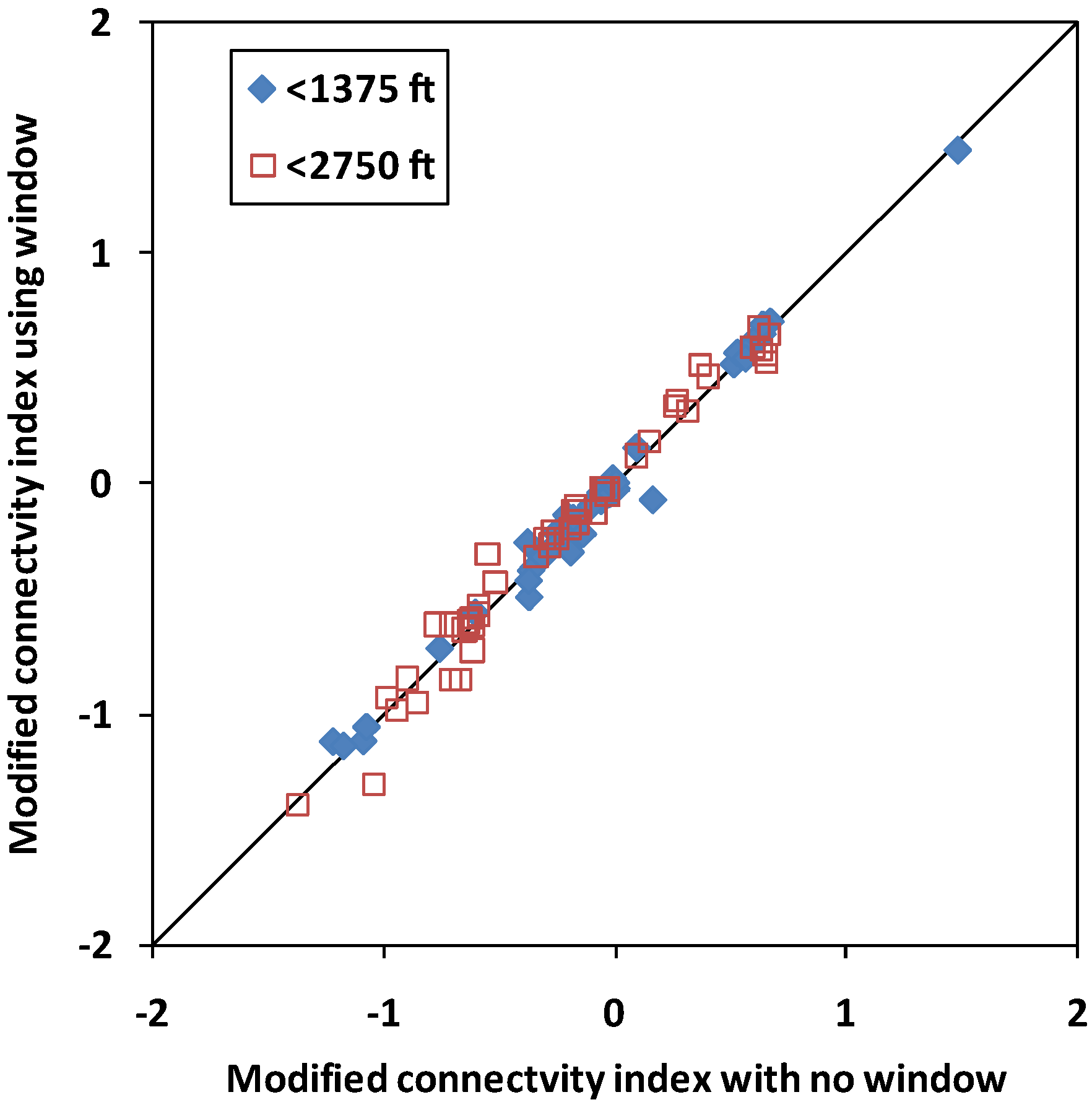
R2 values of the predicted production rates and injectors’ BHPs slightly increased to 0.9964 and 0.9993, respectively. Both window sizes were able to predict the reservoir performance well. However, comparing the modified connectivity indices for the large and small windows with the true ones (obtained from the model with no window), we observed the large window better reveals the heterogeneity than the smaller one (
Figure 18). The CPU time for case of no window was 20 times greater than the time using the large window and 150 times more than the time required when using the small window. In addition, we applied a three window pattern (similar to
Figure 12) and the results were almost identical to the large window. Similar to Case 4, using both large and small windows in this case showed the estimated
δ´s for the closer wells are more accurate than the
δ´s for the more distant wells (
Table 3 and
Figure 18).
Here, we only investigated cases with up to 41 wells. The reason we have not assessed cases with larger numbers of wells is the computational burden for these cases with larger numbers of wells. For example, for the 25 × 16 case, it took 40 days to calculate the δ´s using a standard PC. Larger numbers of wells need much longer times for estimation of the true δ´s (with no window); but we think our findings based on these two cases, however, can be extended to cases with larger numbers of wells.
Figure 16.
Permeability map of Case 5. The well spacing is 945 ft.
Figure 16.
Permeability map of Case 5. The well spacing is 945 ft.
Figure 17.
The two different window sizes applied for Case 5. For well I01, the larger window includes five more wells.
Figure 17.
The two different window sizes applied for Case 5. For well I01, the larger window includes five more wells.
Figure 18.
The modified connectivity indices estimated by the large window (a) are more accurate than the ones obtained by the smaller window (b).
Figure 18.
The modified connectivity indices estimated by the large window (a) are more accurate than the ones obtained by the smaller window (b).
Table 3.
Comparison of R2 values for the Case 5 estimated modified connectivity indices with and without using window of size 2750 ft (small) and 3520 ft (large).
Table 3.
Comparison of R2 values for the Case 5 estimated modified connectivity indices with and without using window of size 2750 ft (small) and 3520 ft (large).
| | <1375 ft | <2750 ft |
|---|
| Small window | 0.77 | 0.58 |
| Large window | 0.87 | 0.70 |
For the cases above we observed that the windowing technique could effectively reduce the number of parameters and the reduced model still contains the most important heterogeneity information and prediction ability. In particular, the estimated modified connectivity indices for the neighboring wells from all the cases are in good agreement with the ones obtained with now window. However, here we only considered the distance and location of the wells as a parameter to select the window shape and size. For further development of this approach, defining criteria to select window size and shape based on the geological and engineering information is needed.


