Turbulent Flow Inside and Above a Wind Farm: A Wind-Tunnel Study

Abstract

Wind-tunnel experiments were carried out to better understand boundary layer effects on the flow pattern inside and above a model wind farm under thermally neutral conditions. Cross-wire anemometry was used to characterize the turbulent flow structure at different locations around a 10 by 3 array of model wind turbines aligned with the mean flow and arranged in two different layouts (inter-turbine separation of 5 and 7 rotor diameters in the direction of the mean flow by 4 rotor diameters in its span). Results suggest that the turbulent flow can be characterized in two broad regions. The first, located below the turbine top tip height, has a direct effect on the performance of the turbines. In that region, the turbulent flow statistics appear to reach equilibrium as close as the third to fourth row of wind turbines for both layouts. In the second region, located right above the first one, the flow adjusts slowly. There, two layers can be identified: an internal boundary layer where the flow is affected by both the incoming wind and the wind turbines, and an equilibrium layer, where the flow is fully adjusted to the wind farm. An adjusted logarithmic velocity distribution is observed in the equilibrium layer starting from the sixth row of wind turbines. The effective surface roughness length induced by the wind farm is found to be higher than that predicted by some existing models. Momentum recovery and turbulence intensity are shown to be affected by the wind farm layout. Power spectra show that the signature of the tip vortices, in both streamwise and vertical velocity components, is highly affected by both the relative location in the wind farm and the wind farm layout.

1. Introduction

Enormous efforts are being carried out to reduce our global dependence on fossil fuels due to their harmful effects on the environment and their non-renewable character. In that context, wind power is one of the most attractive alternatives of renewable and clean sources of energy due to its vast potential and availability [1]. Although a number of wind farms are currently in operation, there are fundamental issues that need to be addressed in order to satisfy the increasing demand for larger, more reliable, and more efficient wind farms. For instance, velocity deficit and turbulence levels in the wake of wind turbines are aspects of special relevance in the process of determining the optimum wind farm layout. Because the turbulent flow inside a wind farm is characterized (among other factors) by the co-existence and superposition of multiple wakes, power losses due to wake effects can reach easily 10%–20% of the total power [2]. Turbulence intensity, another common aspect of interest, is associated directly with fatigue accumulations in the turbines [3] and, as pointed out by Van Binh et al. [4], also plays a direct role on the forces and bending moments acting on the wind turbines. In spite of its importance, there is no well-validated model for the prediction of the spatial distribution of turbulence intensity inside wind farms [5]. Intensive research, both numerically and experimentally, has been carried out to better understand these aspects [6,7,8].

Another subject of special concern is the potential effect of large wind farms on local meteorology. Results from numerical experiments [9] and field measurements [10] suggest that turbulence generated by wind turbines can enhance vertical mixing of momentum, heat, and scalars, leading to substantial changes in near-surface air velocity and temperature. This influence becomes regional as the size of wind farms increases [11]. More recent large-eddy simulations have also shown that under stably-stratified conditions, wind farms can lead to a warming up of the relatively shallow boundary layer flow and a reduction in the magnitude of the surface heat flux [12].

A detailed characterization of the turbulent flow in a wind farm is a challenging task. The coexistence of multiple and superimposed wakes, the effects of the boundary layer, local topology, turbulence levels, and thermal stratification, among other factors, inhibit the understanding of that particular turbulent flow. Theoretical studies have focused on the characterization of the flow inside a wind farm. Most of those studies consider the flow far away from the boundary effects, so that flow properties can be considered adjusted (e.g., [13,14,15]). Other approaches focus on the potential large-scale effects imposed by a large wind farm by considering the overall wind farm as an added surface roughness (e.g., [16]).

Overall, the great complexity of the flow in a wind farm limits our ability to correctly predict the performance and structural stability of the individual turbines. Although numerical simulations are a promising way to address this issue, their limitations (e.g., parameterization uncertainties, resolution) suggest the need for complementing their use with additional/alternative approaches. Field and wind tunnel experiments play a key role in studying the interactions between the atmospheric boundary layer and wind turbines and wind farms. In particular, wind tunnel experiments offer valuable insights about the turbulent flow structure in wind farms under controlled conditions. Early experiments of Milborrow [17] focused on the average efficiency of an array of wind turbines. Corten et al. [18] investigated average velocity profiles above a large wind farm. They found that classical wind farm models often overestimate the efficiency of large wind farms by assuming that the wind turbine wakes do not build up after a few rows down the farm. More recently, Cal et al. [19] and Lebón et al. [20] characterized the flow inside and above a 3 × 3 array of wind turbines.

In spite of the various efforts to characterize the turbulent flow inside and above wind farms, we have limited understanding of how the flow adjusts as it progresses inside wind farms, and how that adjustment affects turbulent transport of momentum and scalar. Certainly, a better understanding of these phenomena would help in the optimization of wind farm layouts, and also in the development of more accurate parameterizations of wind farm effects in large-scale atmospheric models.

In this study, we attempt to contribute to the understanding of the turbulence structure of the flow inside and above a large wind farm. Results are presented from wind-tunnel experiments carried out using a 10 by 3 array of aligned model wind turbines under two different spatial configurations. The wind-tunnel experiments are presented in Section 2. Section 3 shows the flow characterization inside and above the wind farm, and a summary is given in Section 4.

2. Experimental Set-Up

A 10 by 3 array of model wind turbines, aligned with the mean flow, was placed in the thermally stratified boundary-layer wind tunnel of the Saint Anthony Falls Laboratory at the University of Minnesota with the goal of studying turbulence characteristics of the flow inside and above the wind array. The model wind farm was placed in a boundary layer developed over a smooth surface under neutrally-stratified conditions. The boundary-layer wind tunnel has a plan length of 37.5 m with a main test section fetch of roughly 16 m and a cross section of 1.7 m × 1.7 m. There is a contraction with a 6.6:1 area ratio upwind of the test section along with flow conditioning/turbulence control consisting of a coarse wire mesh and honeycomb flow-straightener. The tunnel is driven by a 200 horse-power fan and is operated as a closed return loop. Turbulence intensity in the centre (free stream) of the wind tunnel is approximately 1% for a 2.5 ms${}^{-1}$ free-stream velocity. More details on the wind tunnel can be found in [21,22].

Neutral conditions in the wind tunnel are sustained by controlling both the air and floor temperatures. The floor of the test section consists of heated exchangers made of aluminium plates 0.3 m long and 25.4 mm thick through which a solution of 30% ethylene glycol was circulated. In addition, a heat exchanger was used to control the temperature of the air in the wind tunnel expansion after the fan. Electronic valves were used to automatically control (using a Labview code) the required temperatures of both the air flow and the test section floor with an accuracy of ±0.2 ${}^{\circ }$C.

A turbulent boundary layer was developed with the help of a tripping mechanism (40 mm picket fence) located at the exit of the wind tunnel contraction, where the test section begins. It was allowed to grow in zero pressure gradient conditions by adjustment of the wind tunnel ceiling. The resulting boundary layer has a well-developed surface layer with constant shear stress and a logarithmic velocity profile for the neutral stratification regime.

The experiments were conducted with a free-stream velocity of approximately 3.0 ms${}^{-1}$. A turbulent boundary layer depth of δ ≈ 0.5 m was obtained at the turbine location. The zero pressure gradient boundary layer had a Reynolds number, based on the boundary layer height (δ), of Re${}_{\delta }=U_{\infty }\delta /\nu \approx 1.12\times {10}^5$, and friction velocity of $u_{*}$ = 0.13 ms${}^{-1}$. The aerodynamic surface roughness length was found to be $z_0$ = 0.05 mm. These parameters ($u_{*}$ and $z_0$) were obtained by fitting a logarithmic velocity profile to the measured average velocity in the surface layer (approximately lowest 15% of the boundary layer).

Mean wind velocity in the tunnel free stream was measured using Pitot static tubes (mainly for calibration purposes) and a cross-wire anemometer. The sensor was used to obtain high resolution and simultaneous measurements of two velocity components (streamwise and vertical). The probe is made of 5.0 μm tungsten wires which are connected to an A.A. Lab Systems AN-1003 10-channel CTA/CCA system. During the calibration and measurements the temperature fluctuations were kept within a ±0.2 ${}^{\circ }$C range to avoid bias errors due to thermal drift of the voltage signal. The sensor voltage signatures were sampled at rates of 1 kHz for a measurement period ranging from 60 to 120 s.

Calibration of the cross-wire anemometer was performed at the beginning of each experimental run. Also a post-experiment calibration was carried out to check the validity of the calibration throughout the experiment. The anemometer was calibrated in the free-stream region against a Pitot-static probe, considering seven sensor inclination angles and seven wind velocities at each position. A cubic-spline table calibration method was then used to determine the two instantaneous velocity components from the two instantaneous voltage signatures. For more details on the calibration procedure, see Bruun [23].

The flow around the 10 by 3 wind turbine array was studied under two different layouts. The distance between consecutive wind turbines was set to five and seven rotor diameters ($S_x$ = $\Delta x/d$ = 5 and 7, where d = 0.15 m is the turbine diameter) in the direction of the flow by four rotor diameters in the spanwise direction ($S_y$ = 4). Each model wind turbine consists of a three-blade GWS/EP-6030 × 3 rotor attached to a small DC generator. The turbine angular velocity can be adjusted by changing the resistance of the generator. During the experiments, the tip speed ratio ($\lambda =2\pi r\Omega /\left[60U_{hub}\right]$, where Ω is the angular velocity of the turbine in r.p.m. and $U_{hub}$ = 2.1 ms${}^{-1}$ is the mean velocity at the hub height) was set to approximately 4 for the first row of wind turbines. A similar turbine was used by Chamorro and Porté-Agel [24] to study roughness effects on the turbulent properties of the wake under neutral conditions and by Chamorro and Porté-Agel [25] to study thermal stratification effects on the flow structure in the wake of a wind turbine.

The tip speed ratio is roughly on the order of that observed in field-scale turbines (3.5–8). As shown in Figure 1, the bottom tip of the turbine was set to a height of 0.67 times the turbine radius, which is similar to that found in large-scale turbines (≥2 MW). The turbine rotor was roughly within the lowest third of the turbulent boundary layer. Despite the scaling issues associated with the difference in Reynolds number between the wind-tunnel flow and the atmospheric boundary-layer flow, our measurements provide detailed key information about the behaviour of turbine wakes in turbulent boundary-layer flows. It is also important to note that the high-resolution spatial and temporal measurements presented here can be used to systematically test the performance of numerical models (e.g., LES with different subgrid-scale models and wind turbine forces parameterizations) in the simulation of wind turbine wakes in turbulent boundary-layer flows. Okulov and Sorensen [26] have also showed that, although it is not possible to match the Reynolds number of real wind turbines, it is possible to reproduce the basic characteristics of the wakes (e.g., wake rotation, tip vortices, and helicoidal vortices).

Figure 1. Schematic of the 10 by 3 wind turbine array. Turbine dimensions and measurement locations (top left and bottom), and photograph of the test section with the turbines (top right).

Figure 1. Schematic of the 10 by 3 wind turbine array. Turbine dimensions and measurement locations (top left and bottom), and photograph of the test section with the turbines (top right).

As shown in Figure 1, the cross-wire anemometer was placed at different positions inside the wind farm ($x_i/d=1$, 2,…5, 6, 7; where $x_i$ is the relative downwind distance from the $i^{th}$ turbine, for $i=1$, 2, 3,…7 and 10). At each location, measurements were taken at zero span (y = 0) for elevations ranging from z = 10 mm (= 0.05 H being H the turbine height) to z = 400 mm (= 2 H) every z = 10 mm (= 0.05 H) between z = [0, 1.5] H and z = 20 mm (= 0.1 H) between z = [1.5, 2] H.

3. Flow Characterization

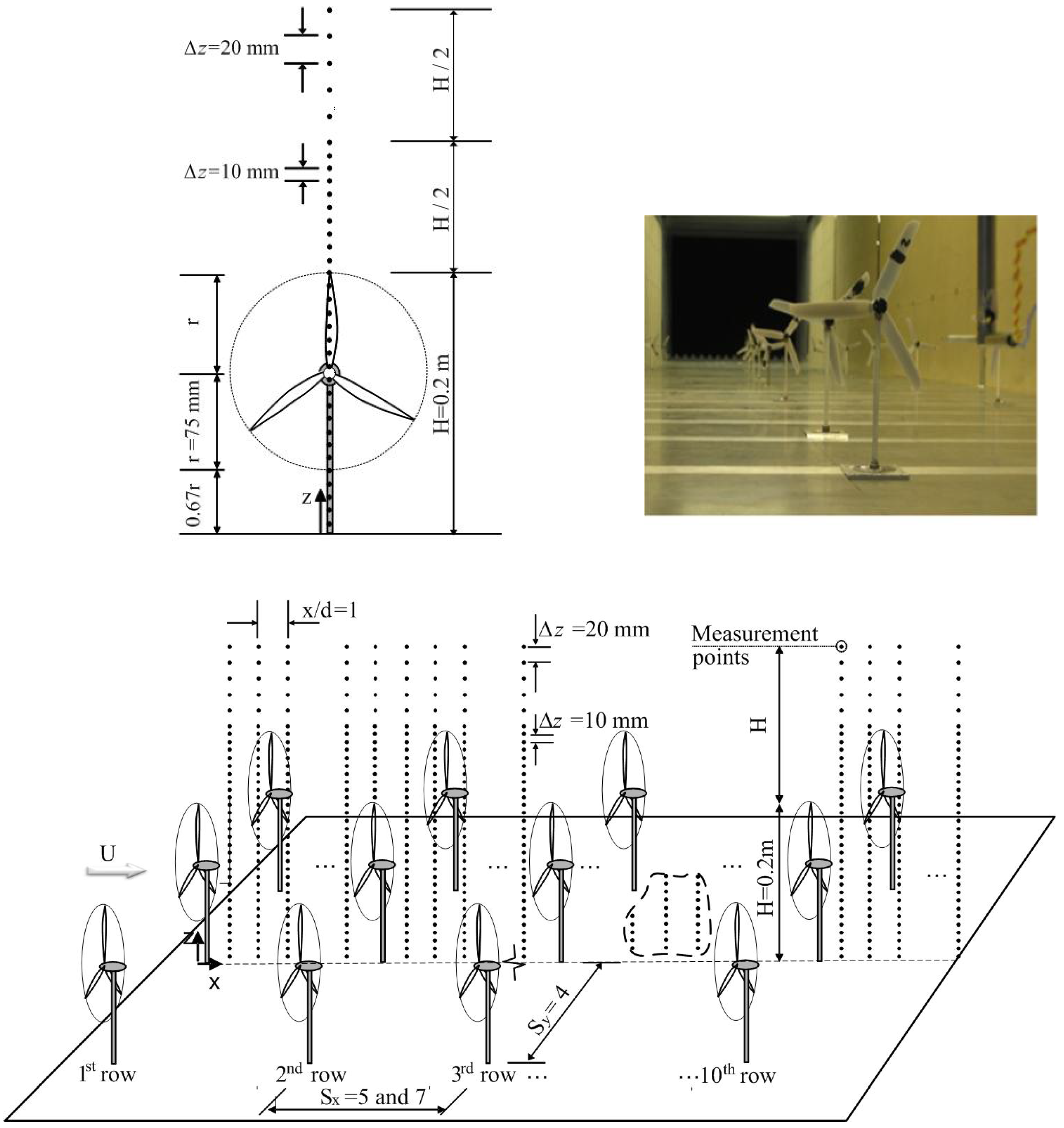
In this section we present flow statistics at different locations inside and above the model wind farm at zero span (see Figure 1) considering two layouts ($S_x$ = 5 and 7 with $S_y$ = 4). Emphasis is placed on the distribution of normalized mean velocity, $U=U_{hub}$ (where $U_{hub}$ is the mean velocity at the turbine hub height), turbulence intensity, $I_u={\sigma }_u/U_{hub}$, kinematic shear stress, $\overline{u^{\prime }{w}^{\prime }}/U_{hub}^2$ and other properties such turbulence energy production, $-\overline{u^{\prime }{w}^{\prime }}\partial U/\partial z$, and velocity spectra.

3.1. Mean Velocity Distribution

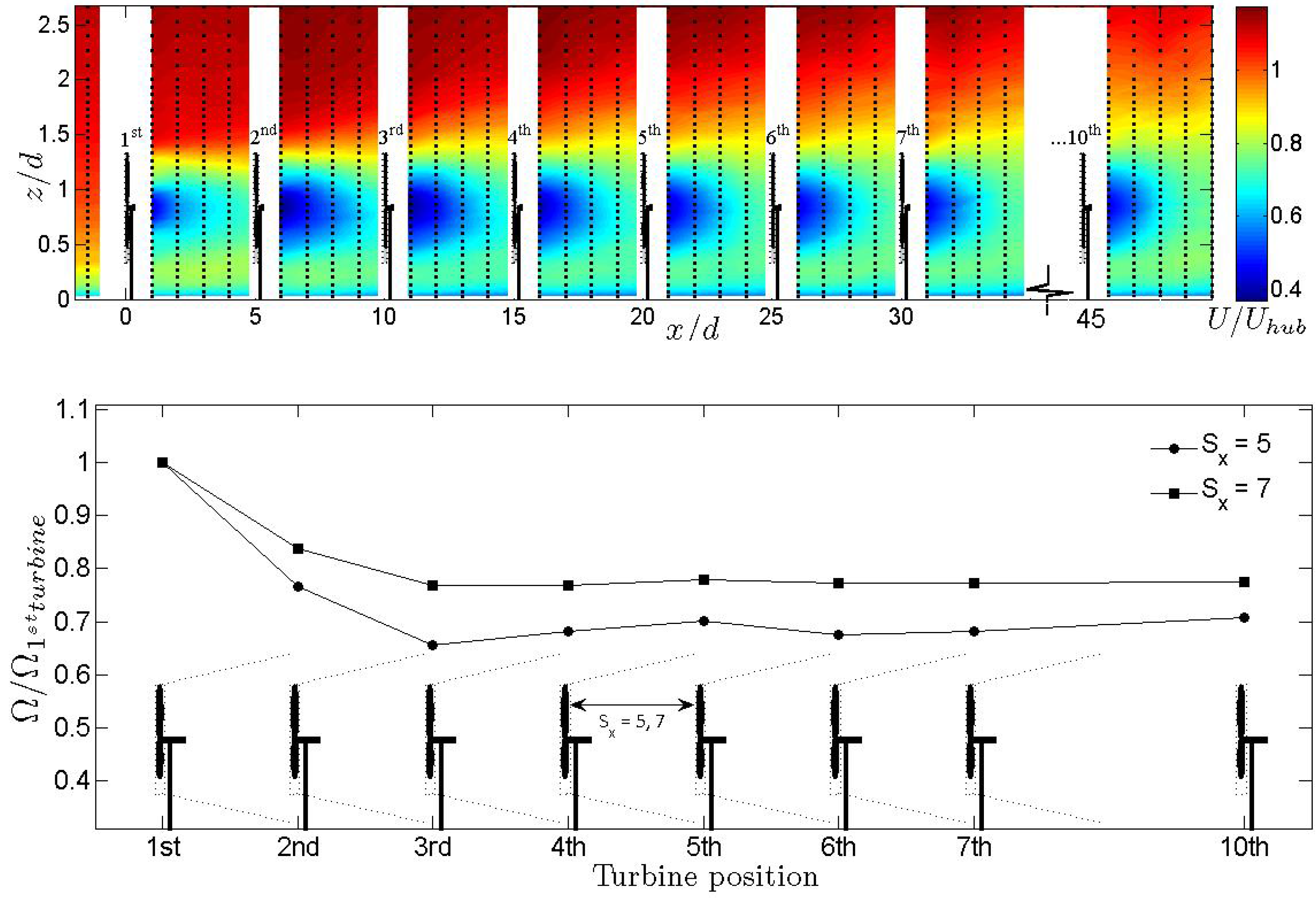
Mean velocity distribution around the wind farm for the case $S_x$ = 5 and $S_y$ = 4 is depicted in Figure 2. Based on the downwind distance required to reach nearly adjusted statistics, our results suggest that the flow can be divided in two broad regions. The first region is located below the wind farm top tip height and has a direct effect on the performance of the wind turbines. In that region, the mean flow appears to reach equilibrium as close as the third to fourth wind turbine row. The second region is located right above the first region and flow adjustment is slower.

Figure 2. Non-dimensional distribution of mean velocity around the wind farm with $S_x=5$ (top) and normalized angular velocity distribution of the different wind turbines with $S_x=5$ and $S_x=7$ (bottom). Dots indicate measurement locations.

Figure 2. Non-dimensional distribution of mean velocity around the wind farm with $S_x=5$ (top) and normalized angular velocity distribution of the different wind turbines with $S_x=5$ and $S_x=7$ (bottom). Dots indicate measurement locations.

The fast velocity adjustment observed below the turbines top tip (hereon region I) is responsible for the relatively quick adjustment of the wind-turbine angular velocities as close as the third row of turbines in the wind farm (see Figure 2). Indeed, minor changes of angular velocity are observed after the third-fourth row of wind turbines for each of the two layouts considered ($S_x$ = 5 and 7). The differences observed in the distribution of angular velocity in the two cases (roughly 8%) suggest that the total power of the wind farm is very sensitive to the geometrical layout. 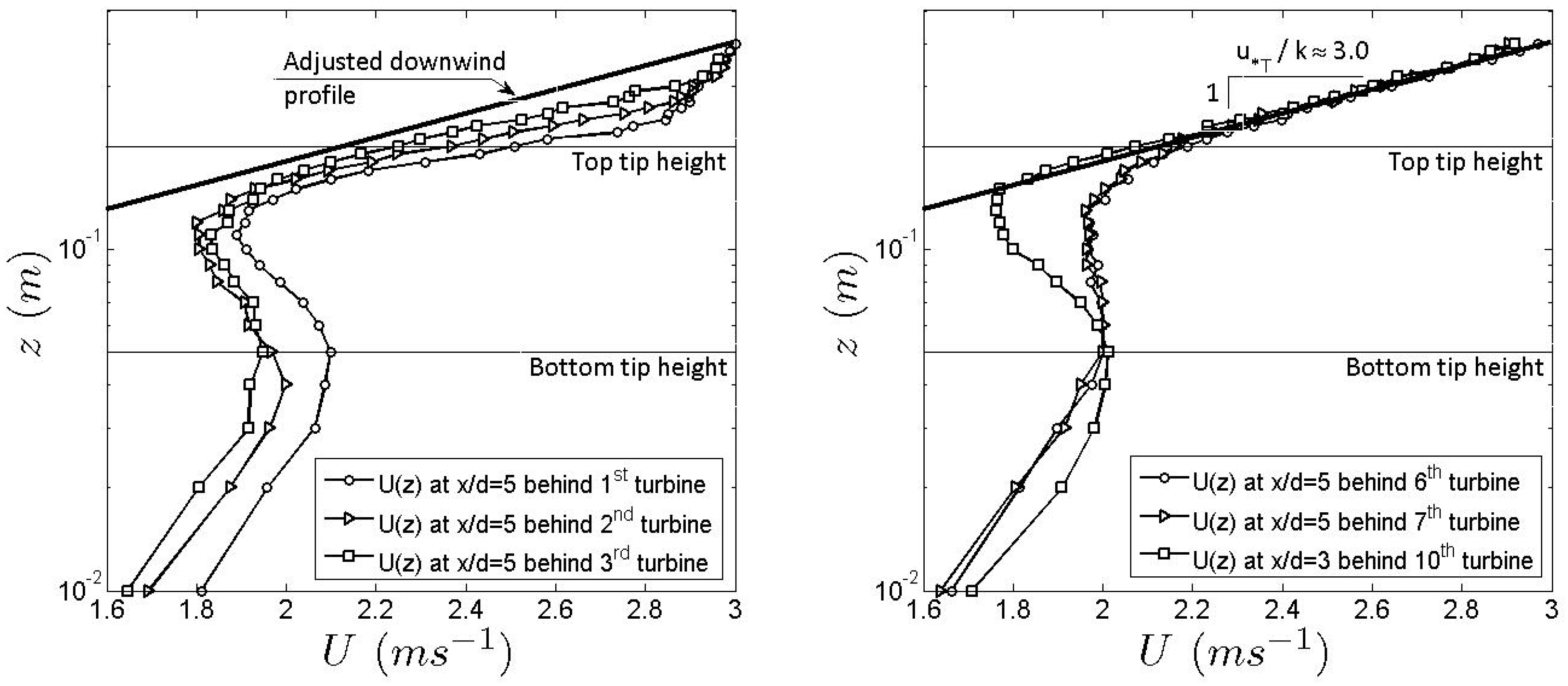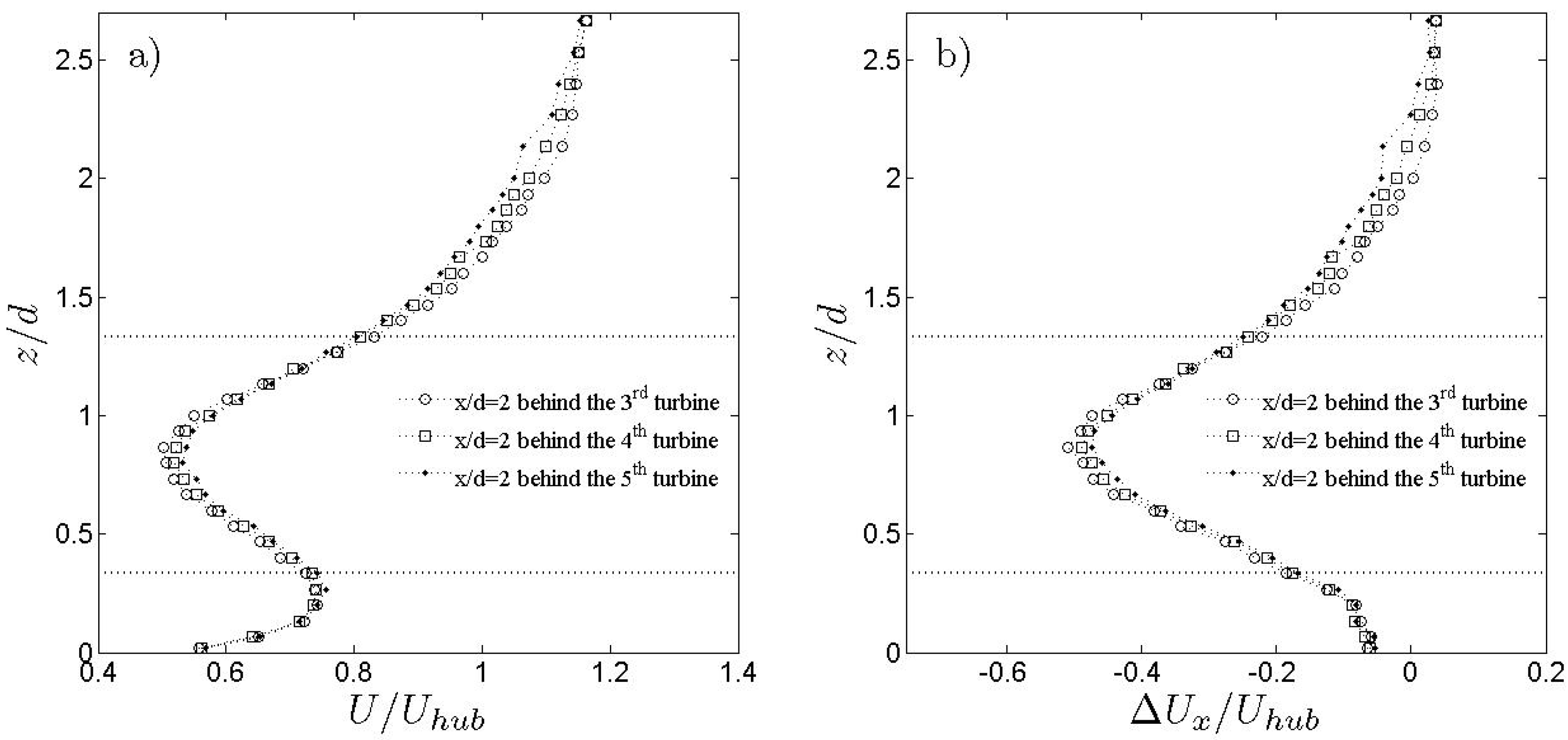Selected vertical velocity profiles at $x/d$ = 2 behind the third, fourth and the fifth row of wind turbines, shown in Figure 3, reveal the fast adjustment of the mean velocity below the top tip height. In contrast, above the top tip (hereon region II) velocity profiles appear to be far from equilibrium, evidencing different mechanisms of mixing and transport of the mean flow between the two regions.

Figure 3. Normalized streamwise velocity component distribution (left) and its deficit (right) in the wind farm.

Figure 3. Normalized streamwise velocity component distribution (left) and its deficit (right) in the wind farm.

The non-axisymmetric shape of the velocity profile observed in region I, induced by the boundary layer (see Figure 3a, complicates its parameterization. As pointed out by Chamorro and Porté-Agel [25], the mean velocity deficit $(\Delta U_x=U-U_{incoming})$ in the wake of a single wind turbine placed in a boundary layer flow is approximately axisymmetric. Due to the interaction of the multiple (superimposed) wakes and the boundary condition imposed by the surface, which limits the wake expansion, the velocity deficit ($\Delta U_x$) is not strictly symmetric below the bottom tip and above the top tip heights. Between those heights, the velocity deficit shows a reasonable symmetric shape.

Although different approaches have been proposed to estimate the mean velocity inside a wind farm, they unfortunately do not fully consider the boundary layer effects. Similar to the velocity deficit formulation downwind of a single wind turbine, suggested by Chamorro and Porté-Agel [25], the velocity deficit in an aligned wind farm can bee described by

$$\Delta U_x(x,r){{|}_i=\Delta U_{hub}\left(x\right)|}_{i}f(r/R)$$

(1)

where $\Delta U_x{(x,r)|}_i$ is the velocity deficit in the wake of the $i^{th}$ row of wind turbines, $\Delta U_{hub}{\left(x\right)|}_i$ is its counterpart at the hub height, r is the distance from the center of the wake and R is the characteristic width of the wake at distance x downwind of the rotor. Because the mean velocity adjusts relatively fast (see Figure 2), Equation (1) becomes quickly independent of the relative position i in the farm.

Figure 4 shows clearly that the mean velocity above the top tip height (region II) adjusts far inside the wind farm. The velocity appears to reach equilibrium starting from the sixth row of wind turbines, and upwind of this location, the flow is transitioning. The relative location where the flow reaches equilibrium is of special importance. For instance, large-scale atmospheric models require the specification of the additional surface roughness induced by a wind farm. That parameter should be obtained under equilibrium conditions, where similarity theory can be applied. In general, a departure of the log-law velocity distribution is expected downwind of a surface roughness transition. Indeed, both mean velocity and surface shear stress adjust slowly downwind of a transition [27,28]. Because the transition zone appears to be significant in the wind farm (6–7 turbine rows), its characterization is relevant in the understanding of the interaction between the wind farm and the boundary layer, which ultimately modulates the power available for the wind turbines.

Figure 4. Non-adjusted (left) and adjusted (right) velocity distributions above the top tip in the wind farm at different locations ($S_x=5$). Horizontal lines represent the turbine bottom and tip heights.

Figure 4. Non-adjusted (left) and adjusted (right) velocity distributions above the top tip in the wind farm at different locations ($S_x=5$). Horizontal lines represent the turbine bottom and tip heights.

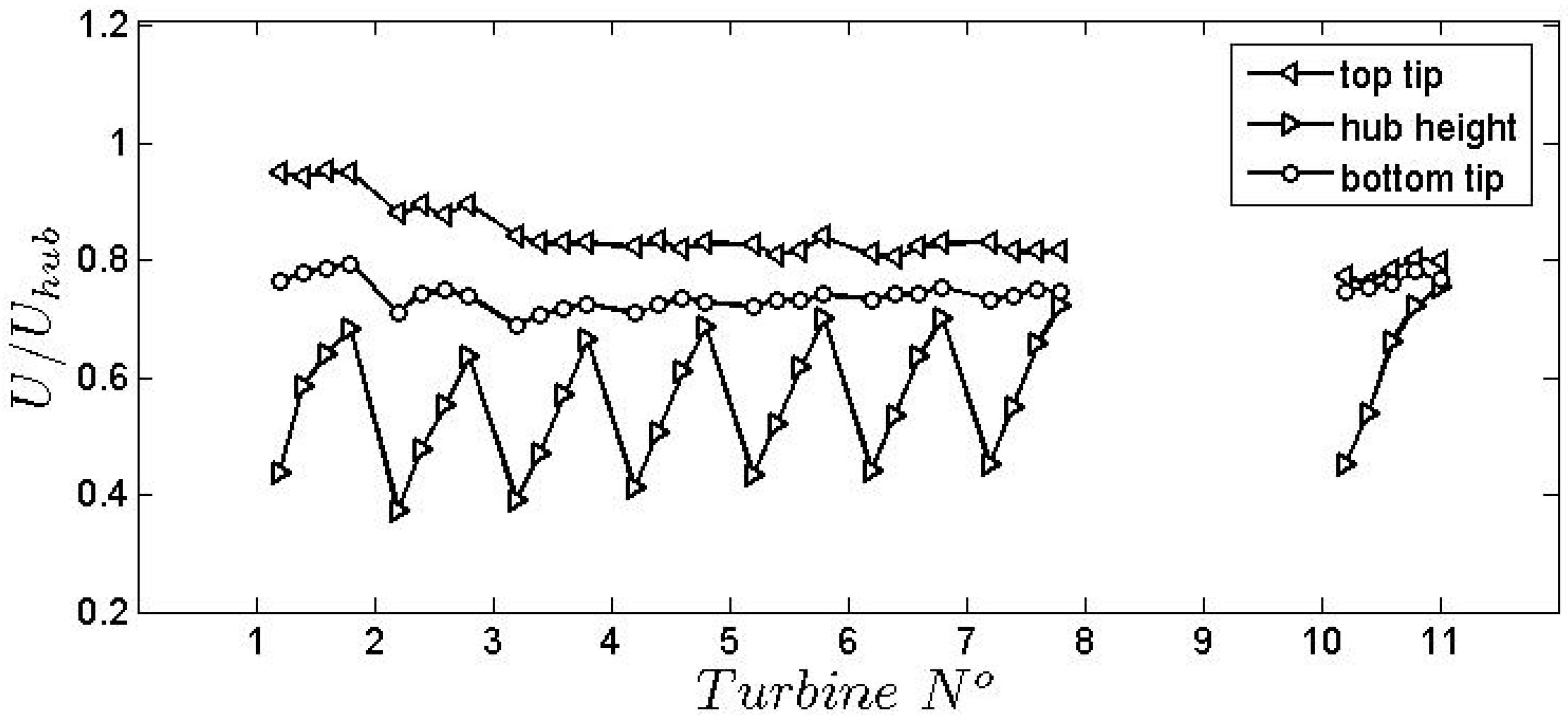
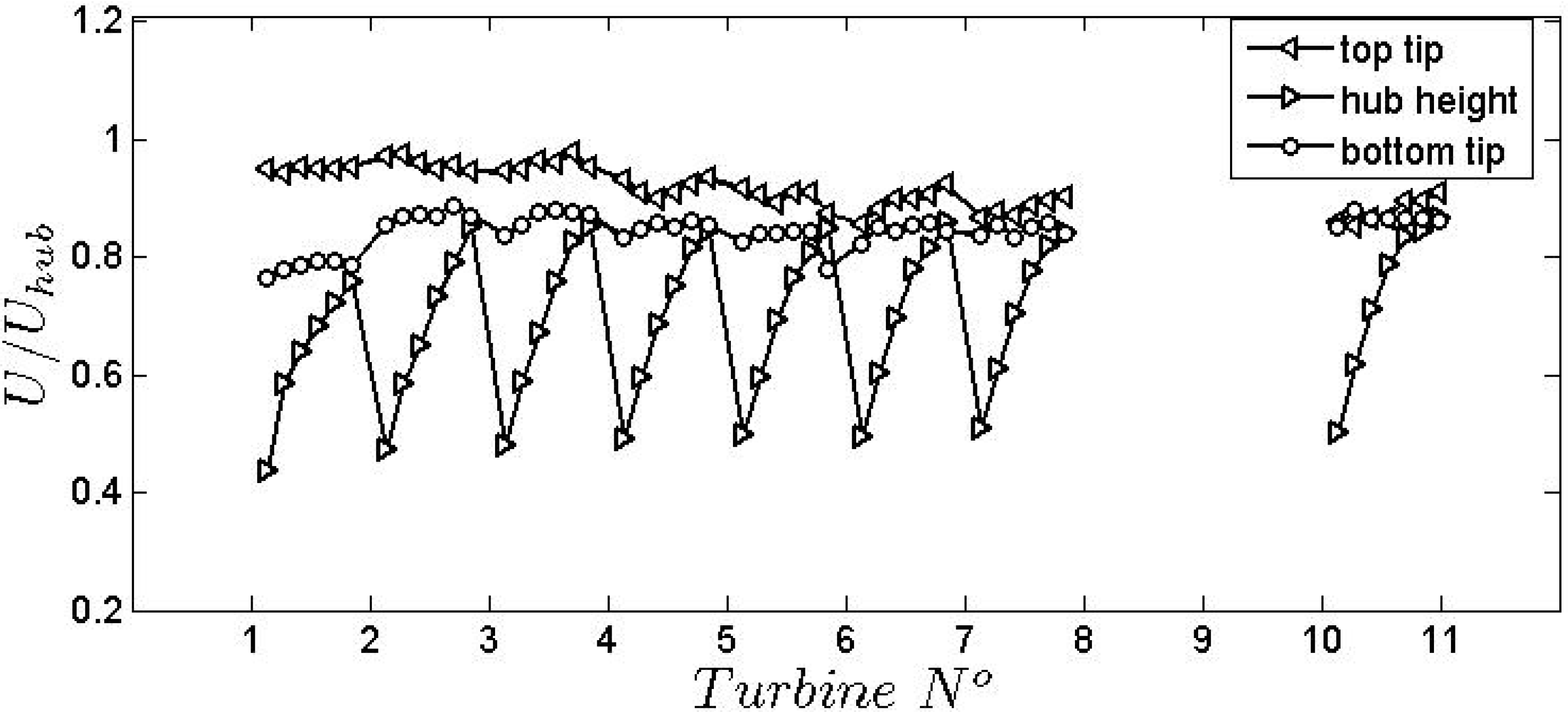
A representative characterization of the mean flow at the bottom tip, hub, and top tip heights in region I throughout the wind farm is given in Figure 5. From that figure it is clear that the momentum recovery between the wind turbines is insufficient, especially in the case of $S_x$ = 5. The velocity at the bottom and at the top tip heights shows much less variation. The mean flow appears to be more uniform directly upstream of each turbine in the case of $S_x$ = 7. Again, this effect remarks the importance of wind farm layout in the overall wind farm performance.

Figure 5. Normalized streamwise velocity component distribution in the wind farm. $S_x=5$ (top) and $S_x=7$ (bottom).

Figure 5. Normalized streamwise velocity component distribution in the wind farm. $S_x=5$ (top) and $S_x=7$ (bottom).

3.2. Turbulence Intensity Distribution

In general, turbulence intensity in the wake of a wind turbine, $I_{wake}$ , comes from two main sources: the background turbulence, $I_0$ , and the wake added turbulence, $I_{+}$ . They are related in the following way:

$$I_{wake}^2=I_0^2+I_{+}^2$$

(2)

Several empirical expressions have been proposed to estimate the added turbulence intensity $I_{+}$ [29,30,31]. Recently, Chamorro and Porté-Agel [24] showed that the use of a single value to represent the wake-averaged added turbulence intensity is not sufficient due to its high spatial variability. In a simple attempt to include the non-axisymmetric effects, Chamorro and Porté-Agel [24] propose to differentiate between a positive change (increase) $I_{+}^{+}$, which occurs at the upper part of the wake, and a negative change (decrease) $I_{+}^{-}$ in the lower part of the wake.

For a wind farm configuration where multiple turbine wakes coexist, Frandsen and Thogersen [32] proposed a model that considers the wind farm layout. It is based on the geostrophic drag law and takes into account the additional surface roughness generated by the turbines:

$$I_{+}=\frac{1}{2}(I_0+\sqrt{I_0^2+I_{++}^2})$$

(3)

where

$$I_{++}=\frac{0.36}{1+0.2\sqrt{(s_{1}s/C_T)}}$$

(4)

Here $C_T$ is the thrust coefficient, $s_1$ and s are the inter-turbine spacings (normalized by the rotor diameter) within a row and between rows, respectively. The Frandsen and Thogersen [32] model applies above the hub height, and has become the European standard.

An alternative model, proposed by Wessel and Lange [33], assumes that the overall turbulence intensity at a particular location in the wind farm is given by:

$$I\left(x\right)=I_0+\sqrt{{\sum }_{i=1}^N{I}_{+i}^2\left(x\right)}$$

(5)

where N is the number of upwind turbines from the location of interest (x) and $I_{+i}$ is the added turbulence intensity contribution of the $i^{th}$ turbine at location x.

Although these models determine a unique representative value for the turbulence intensity in the wind farm, they show fundamental differences. The first approach assumes that turbulence levels do not change with the number of turbines in the wind farm, while the second approach assumes a monotonic increase with the downwind distance in the wind farm. The structural differences given by these approaches point out that, to date, there is no consensus model for the prediction of turbulence intensity inside wind farms [5].

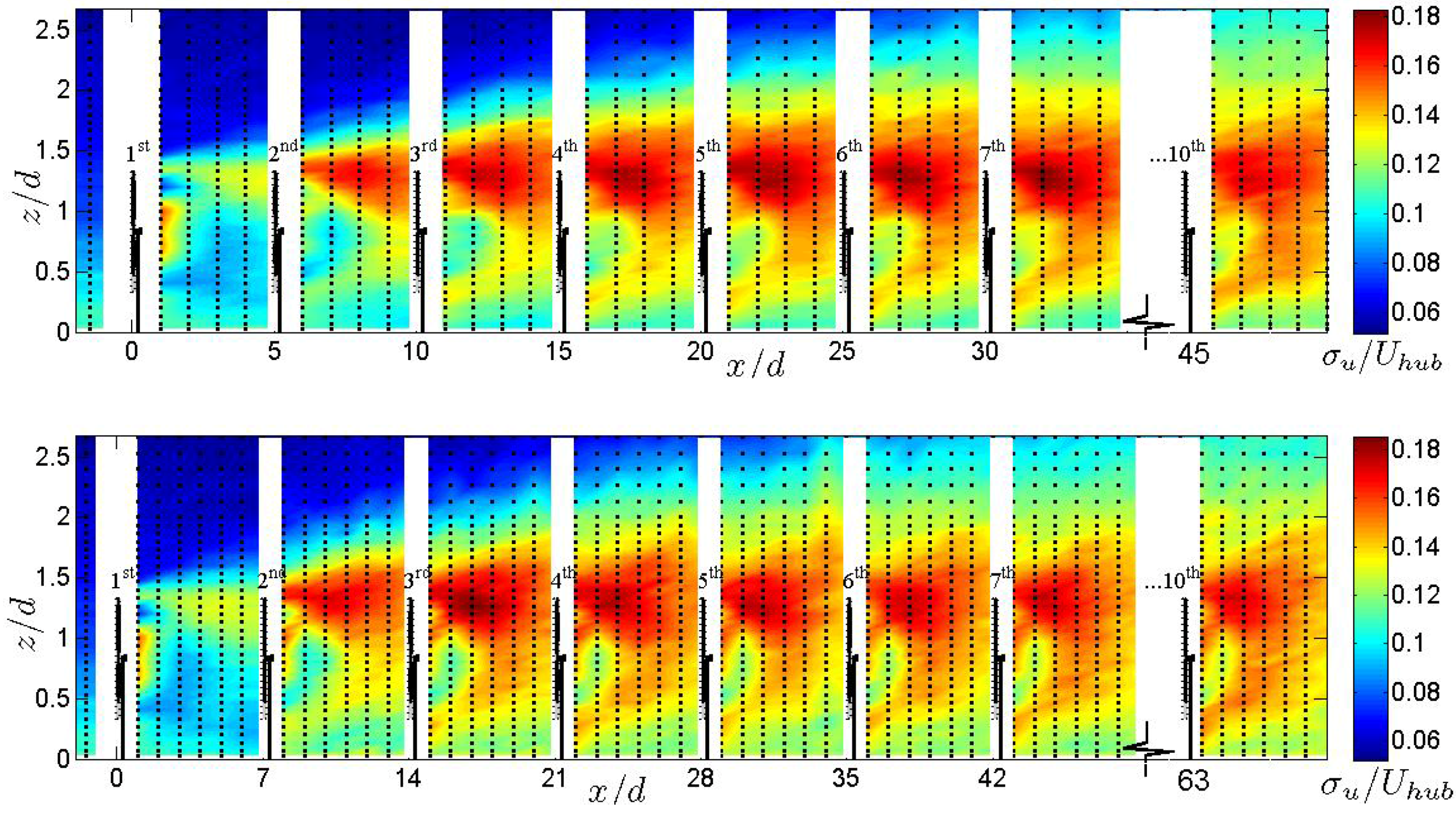
Our results (Figure 6) show that turbulence intensity significantly increases in the first three-four rows of wind turbines and, after the fifth row, it appears to reach a plateau, which differs from the Wessel and Lange [33] model (monotonically positive growth).

Figure 6. Turbulence intensity distribution around the wind farm. $S_x$ = 5 (top) and $S_x$ = 7 (bottom). Dots indicate measurement locations.

Figure 6. Turbulence intensity distribution around the wind farm. $S_x$ = 5 (top) and $S_x$ = 7 (bottom). Dots indicate measurement locations.

Significant differences in the spatial distribution of the turbulence intensity are observed behind a single wind turbine and far inside the wind farm. For instance, from Figure 6 an enhancement of roughly 50% in turbulence intensity is observed between these two situations. Also, an increase of the turbulence levels at the bottom tip height is clearly observed inside the wind farm.

Figure 6 also shows that, after the second row of wind turbines, the peak of turbulence intensity is consistently located near the top tip height at roughly three rotor diameters downwind of each turbine ($x/d$≈ 3). This peak is closer than that observed in a single wind turbine. Wind tunnel experiments performed by Chamorro and Porté-Agel [25] and corresponding large-eddy simulations by Wu and Porté-Agel [34] have shown that maximum values of turbulence intensity in the wake of a single wind turbine are located at a distance of 4 to 5.5 rotor diameters under neutral stratification. Other recent LESs of field turbine wakes show a similar turbulence intensity enhancement at the top tip level, with a maximum value at a downwind distance of about 2–3 rotor diameters [35].

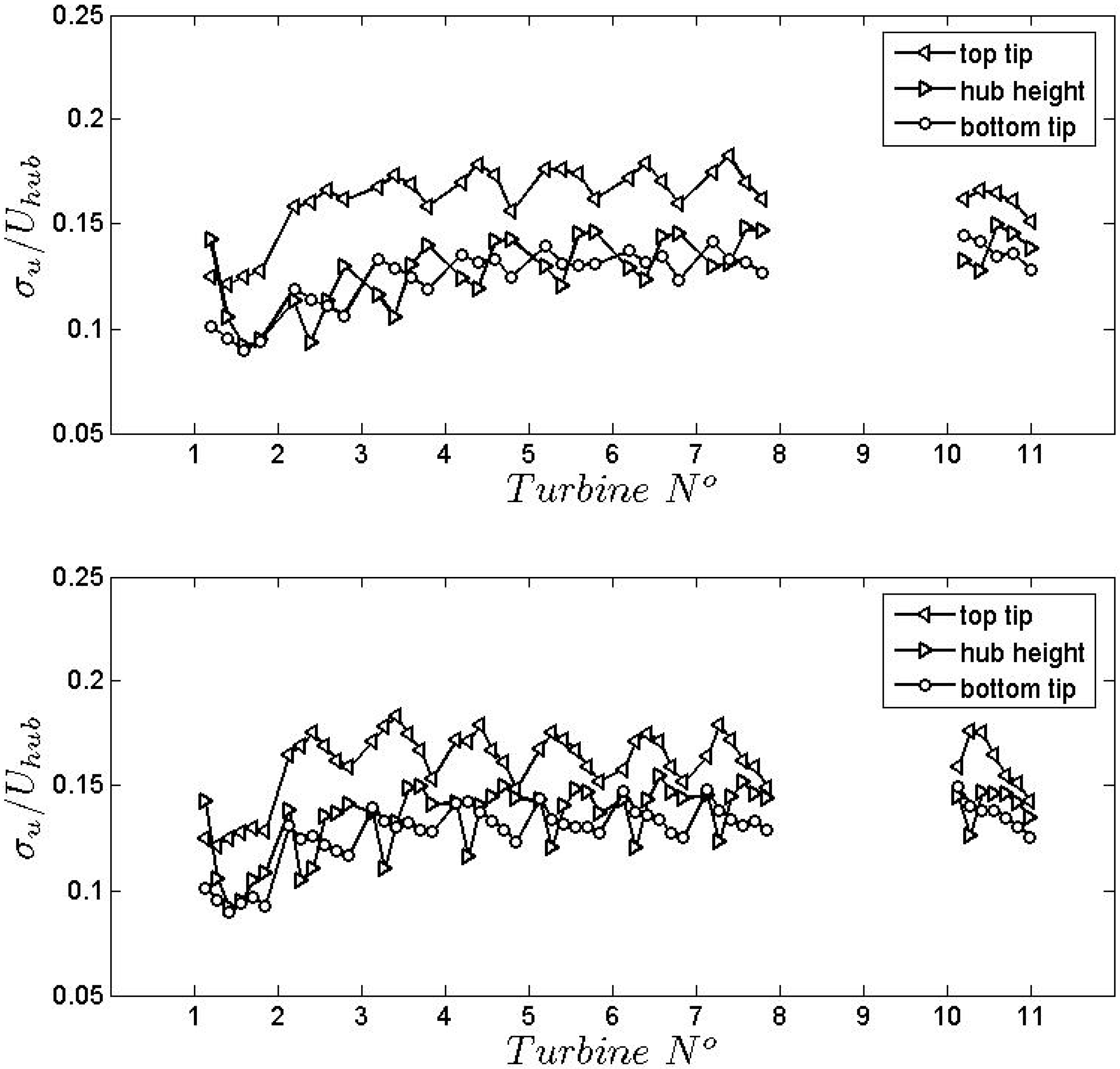
The comparison of the two layouts ($S_x$ = 5 and $S_x$ = 7) reveals that the distribution of turbulence intensity in the vicinity of each wind turbine depends also on the separation between turbines ($S_x$). Figure 7 shows the turbulence intensity at the bottom tip, hub, and top tip heights. It is clearly observed that in both cases the local maximum of turbulence intensity is located around top tip with a peak at a normalized distance of $x/d$ ≈ 3.

Figure 7. Turbulence intensity distribution in the wind farm at bottom, hub and top tip heights. $S_x$ = 5 (top) and $S_x$ = 7 (bottom).

Figure 7. Turbulence intensity distribution in the wind farm at bottom, hub and top tip heights. $S_x$ = 5 (top) and $S_x$ = 7 (bottom).

The gradual adjustment of the mean velocity observed in region II (see Figure 2) is also evident in the case of the turbulence intensity distribution depicted in Figure 6. There, the turbulence intensity gradually transitions to higher levels with downwind distance, forming a clear layer with enhanced turbulence. This is expected since the wake expansion, above the top tip level, and the superposition of multiples wakes produce higher velocity fluctuations.

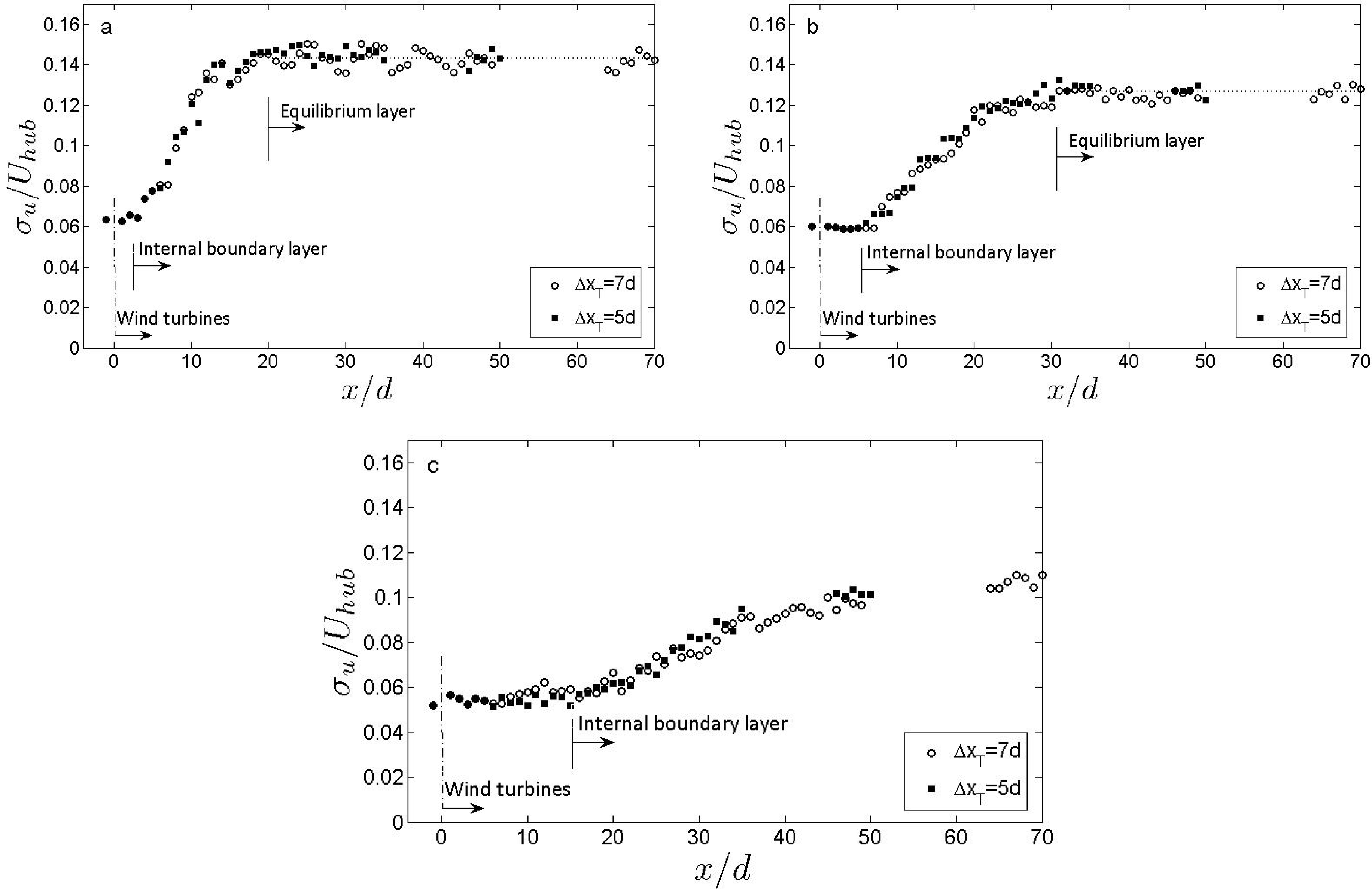
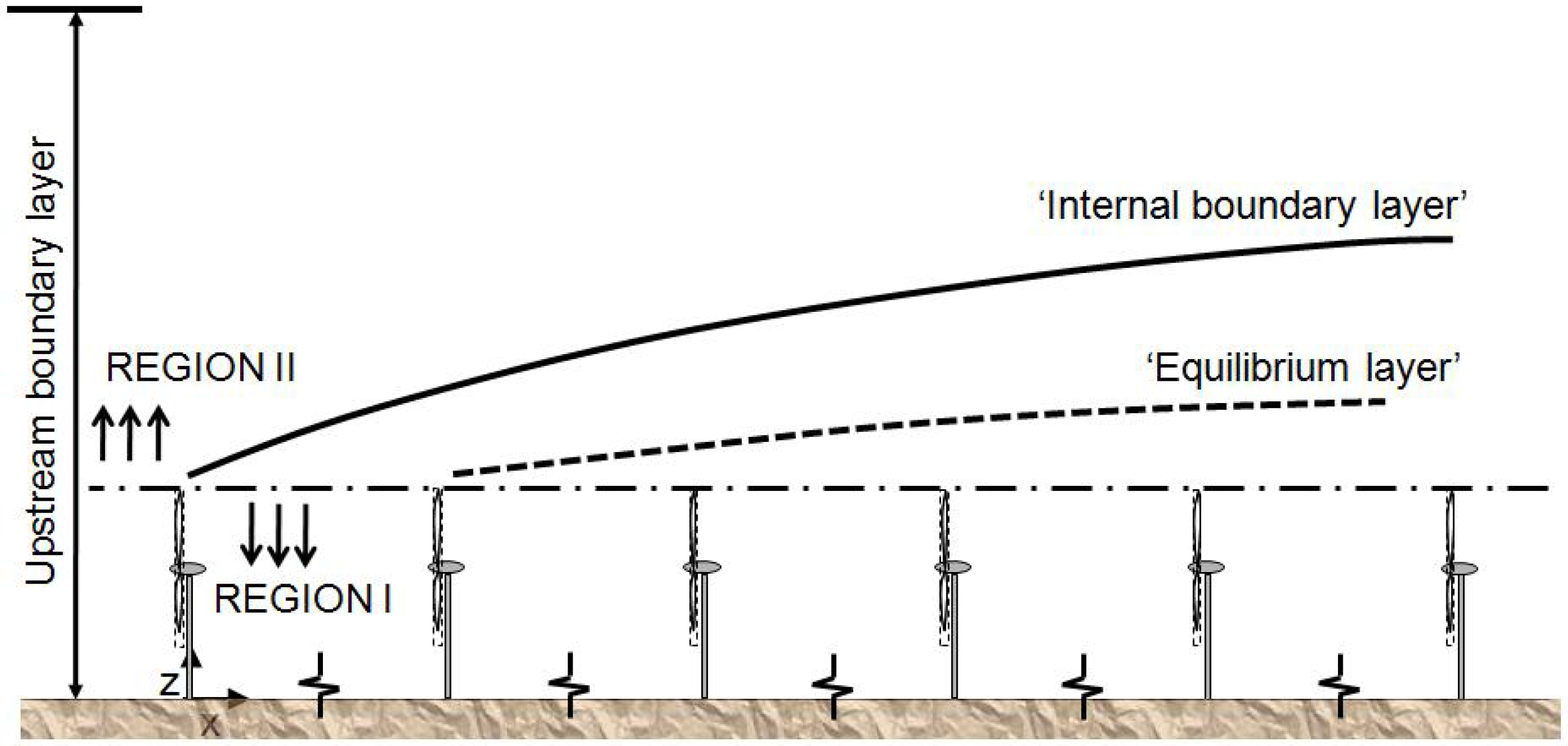
In order to appreciate the relative location of this layer, turbulence intensity is plotted in Figure 8 at several heights (1.25 H; 1.5 H and 2 H, where H is the turbine height) for the two layouts. From that figure, two distinct layers can be distinguished. One layer, an internal boundary layer, is modulated by the interaction between the wind farm and the incoming boundary layer flow. Within the other layer, an equilibrium layer, flow statistics are adjusted to the new conditions imposed by the wind turbines. A schematic of these layers is depicted in Figure 9.

Figure 8. Turbulence intensity distribution at different heights above the wind farm. (a) z = 1.25 H; (b) z = 1.5 H; (c) z = 2 H. H = turbine height.

Figure 8. Turbulence intensity distribution at different heights above the wind farm. (a) z = 1.25 H; (b) z = 1.5 H; (c) z = 2 H. H = turbine height.

Figure 9. Conceptual description of the different regions and layers in a wind farm.

Figure 9. Conceptual description of the different regions and layers in a wind farm.

These characteristic layers are always present in the atmospheric boundary layer after a surface roughness transition. Because velocity and turbulent fluxes are highly modified after a surface transition, accurate parameterizations are of special relevance in large-scale atmospheric models (e.g., weather prediction models). The clear existence of these two layers above the wind farm suggests that, from a large-scale perspective, a finite-size wind farm can be treated as a special case of roughness transition.

3.3. Other Flow Statistics

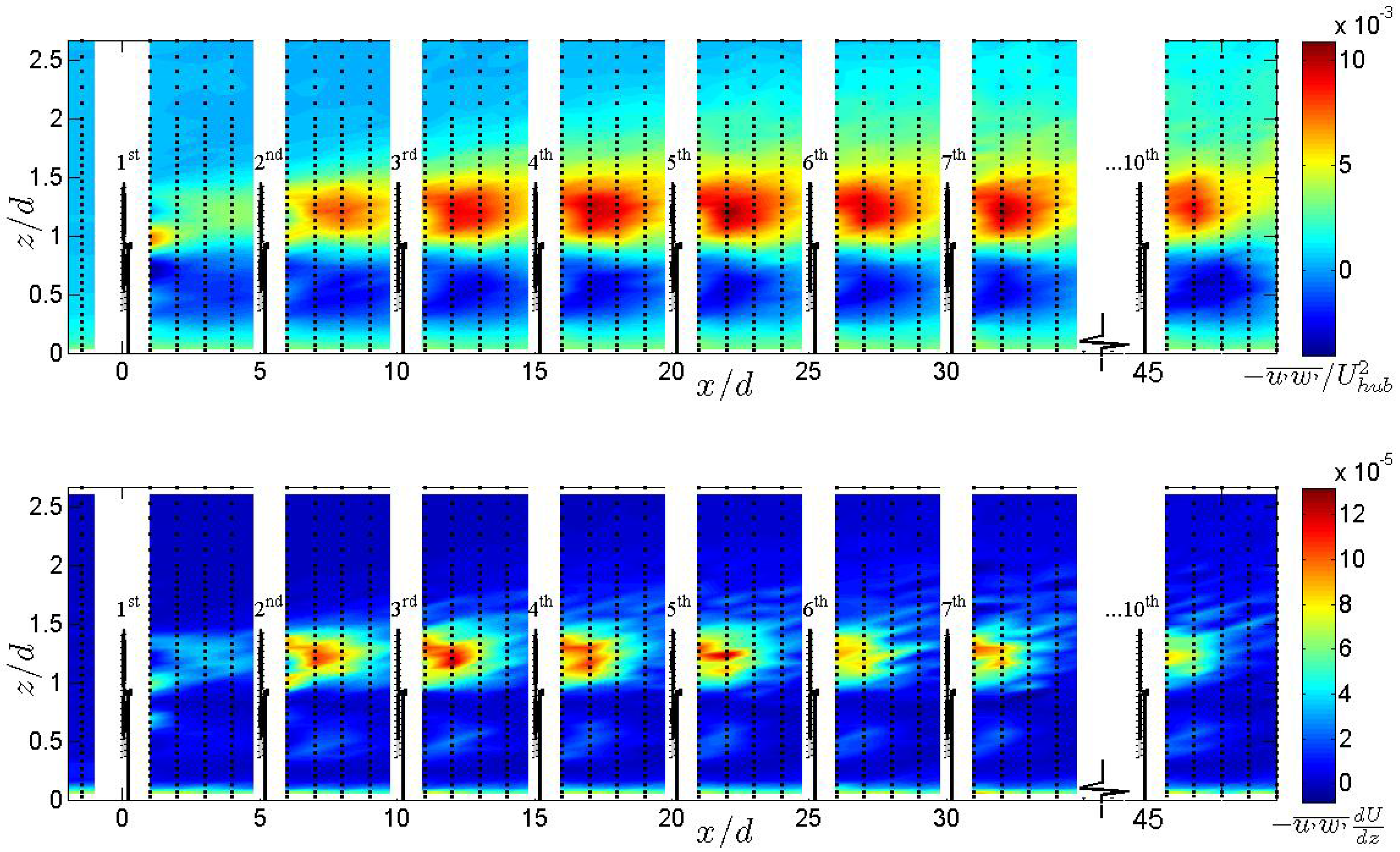
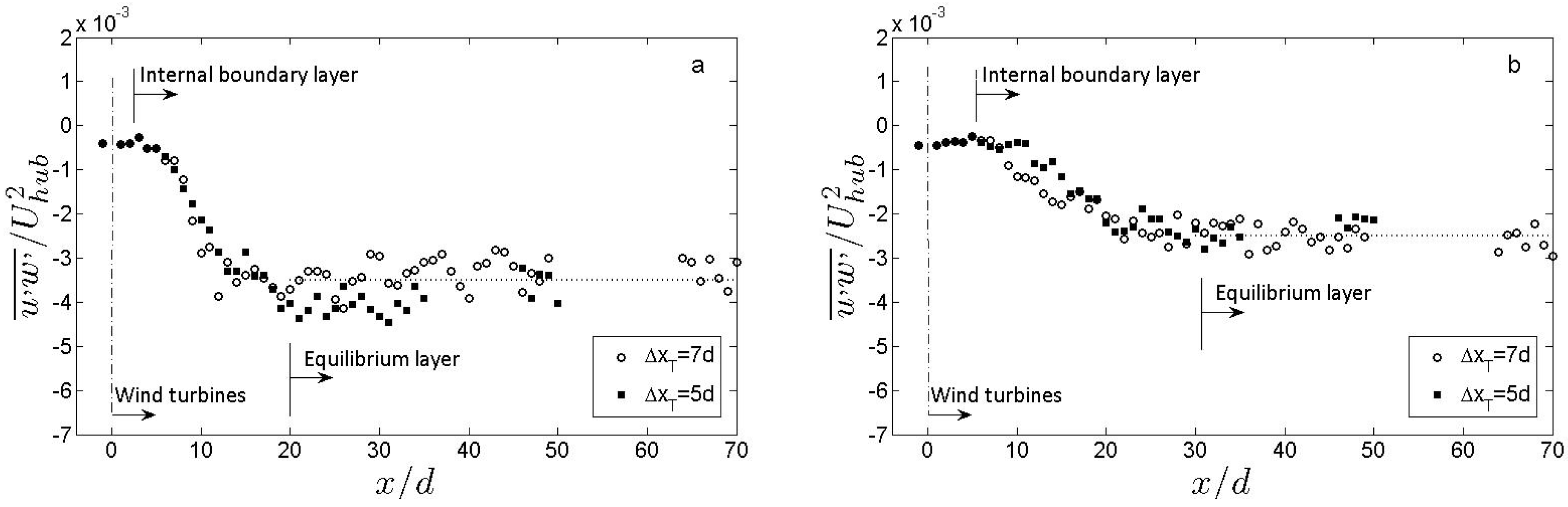
Spatial distribution of normalized kinematic shear stress, $-\overline{u^{\prime }{w}^{\prime }}/U_{hub}^2$, is shown in Figure 10 for the case $S_x$ = 5. An important enhancement of the turbulent stresses is observed up to roughly the fourth row of wind turbines. The enhancement of turbulent stresses is higher with respect to the case of a single turbine scenario (as observed between the first and second wind turbine). Similar to the case of the mean velocity and turbulence intensity, both an internal and equilibrium layer are observed in region II.

Figure 10. Non-dimensional distributions of kinematic shear stress (top) and turbulent kinetic energy production (bottom) inside and above a 10-turbines wind farm ($S_x$ = 5).

Figure 10. Non-dimensional distributions of kinematic shear stress (top) and turbulent kinetic energy production (bottom) inside and above a 10-turbines wind farm ($S_x$ = 5).

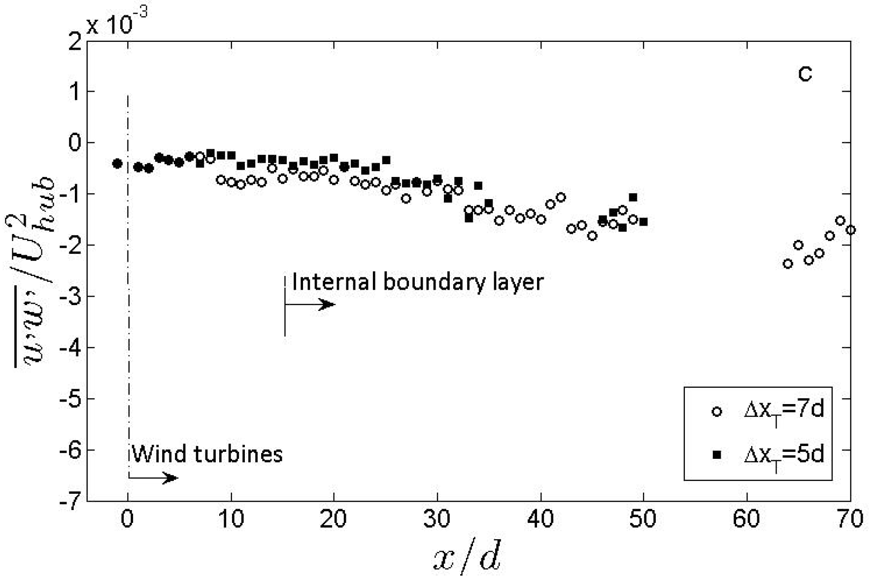
Similar to the case of turbulence intensity (Figure 8), Figure 11 shows the adjustment of the kinematic shear stress in region II with distance at different heights. Both an internal boundary layer and an equilibrium layer are clearly observed. Their specific locations, at a given height, agree with those observed for the turbulence intensity. As expected, high levels of kinematic shear stress are observed closer to the wind turbines.

Figure 11. Non-dimensional distribution of kinematic shear stress at different heights above the wind farm. (a) z = 1.25 H; (b) z = 1.5 H; (c) z = 2 H. H = turbine height.

Figure 11. Non-dimensional distribution of kinematic shear stress at different heights above the wind farm. (a) z = 1.25 H; (b) z = 1.5 H; (c) z = 2 H. H = turbine height.

Areas of greater turbulence energy production ($-\overline{u^{\prime }{w}^{\prime }}\partial U/\partial z$ component) through the wind farm, shown in Figure 10, are consistent with the enhanced levels of turbulence intensity observed above the hub height. Its maximum values are located between one and three rotor diameters downwind of each turbine.

It is important to notice that the highest levels of turbulent kinetic energy production and turbulence intensity do not coincide with the location of the different wind turbines (which normally are 5 to 7 rotor diameters apart). An enhancement of the turbulence energy production is observed also at the bottom tip height for the different wind turbines.

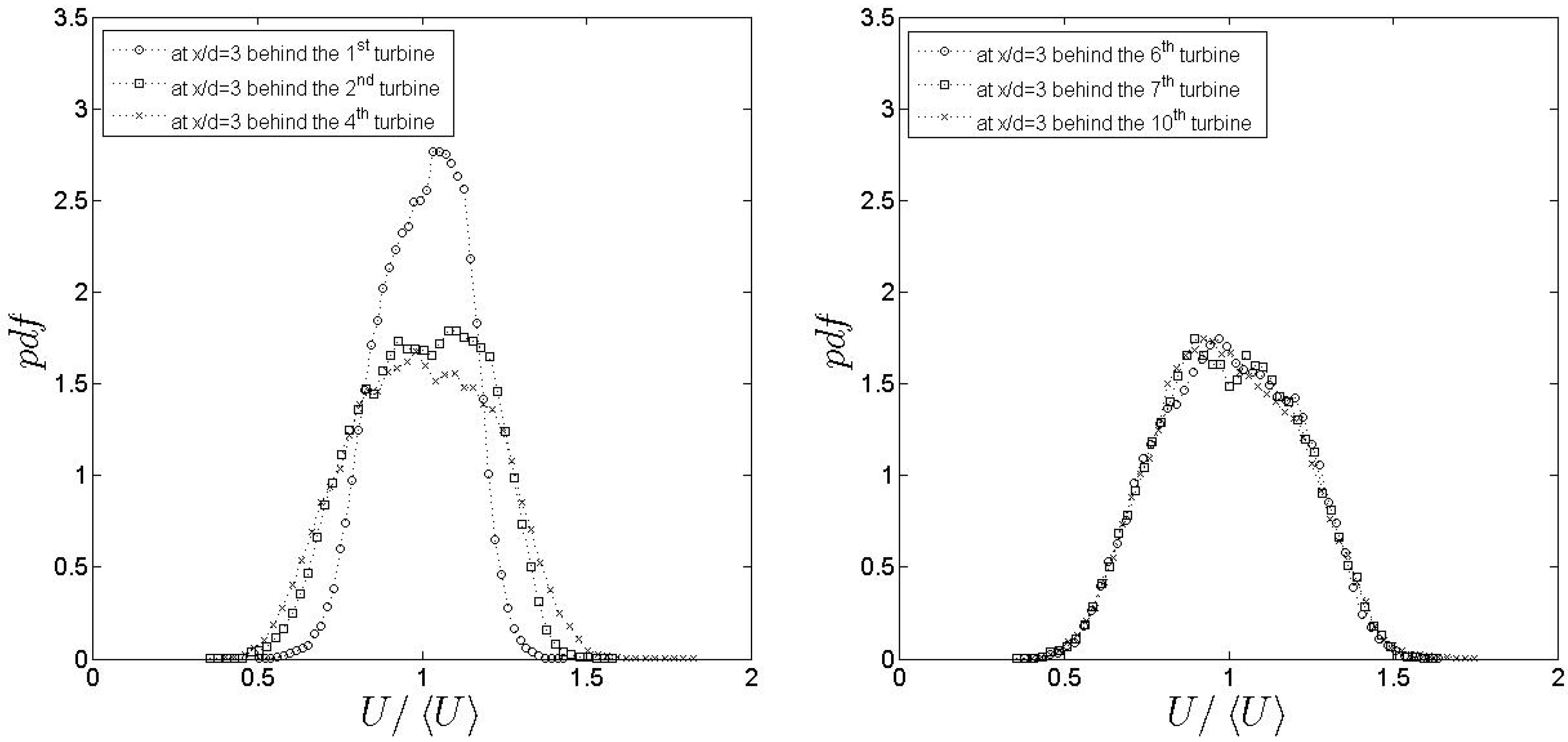
In general, turbulence characteristics at the turbine top tip height are of special relevance. They give insights on the interaction between regions I and II. In particular, from the pdf of the streamwise velocity component at a relative distance $x/d$ = 3 (Figure 12) it is possible to see the adjustment of the flow. It is noted that for the first four wind turbines the velocity distribution is clearly not adjusted.

Figure 12. P.d.f. of streamwise velocity component at top tip height inside the wind farm ($S_x=5$).

Figure 12. P.d.f. of streamwise velocity component at top tip height inside the wind farm ($S_x=5$).

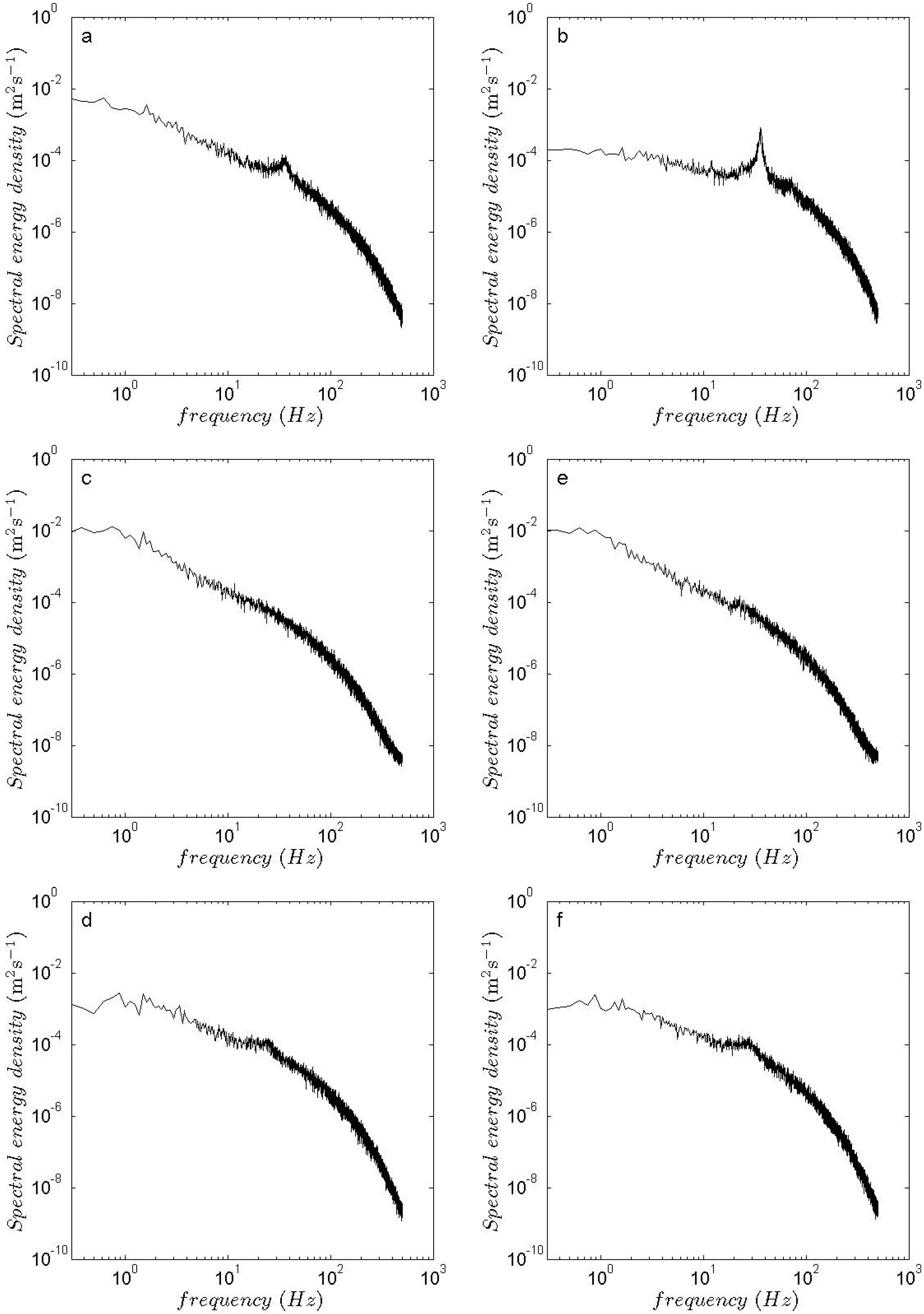
Power spectra of the streamwise and vertical velocity components reveal important effects of the flow turbulence on the helicoidal tip vortices (see Figure 13). In particular, it is observed that behind the first wind turbine, where the background turbulence is relatively low, tip vortices induce a strong signature on the spectrum at a frequency coincident with that of the consecutive blades. Velocity spectrum of the vertical velocity component shows a stronger signature of the tip vortices compared with the streamwise velocity spectrum (see also [27]).

Figure 13. Power spectrum of the streamwise (u) and vertical (w) velocity components at top tip height inside the wind farm. (a) u-component at $x/d$ = 1 behind the 1^st turbine ($S_x$ = 5); (b) w-component at $x/d$ = 1 behind the 1^st turbine; (c) u-component at $x/d$ = 1 behind the 10^th turbine ($S_x$ = 5); (d) w-component at $x/d$ = 1 behind the 10^th turbine ($S_x$ = 5); (e) u-component at $x/d$ = 1 behind the 10^th turbine ($S_x$ = 7); (f) w-component at $x/d$ = 1 behind the 10^th turbine ($S_x$ = 7).

Figure 13. Power spectrum of the streamwise (u) and vertical (w) velocity components at top tip height inside the wind farm. (a) u-component at $x/d$ = 1 behind the 1^st turbine ($S_x$ = 5); (b) w-component at $x/d$ = 1 behind the 1^st turbine; (c) u-component at $x/d$ = 1 behind the 10^th turbine ($S_x$ = 5); (d) w-component at $x/d$ = 1 behind the 10^th turbine ($S_x$ = 5); (e) u-component at $x/d$ = 1 behind the 10^th turbine ($S_x$ = 7); (f) w-component at $x/d$ = 1 behind the 10^th turbine ($S_x$ = 7).

Far inside the wind farm, at a relative distance of $x_{10}/d$ = 1 (i.e., behind the tenth wind turbine), it is possible to notice that, due to the relatively high levels of velocity fluctuations inside the wind farm (case $S_x$ = 5), tip vortices have negligible effects on the streamwise velocity component and minimum effects on the vertical velocity component. On the other hand, the slightly lower turbulence levels around the turbines in the case of $S_x$ = 7 lead to non-negligible signatures of the tip vortices in the power spectrum of both velocity components.

3.4. Wind Farm Roughness

The idea of representing a large wind farm as an added surface roughness to study local meteorology effects in large-scale atmospheric models has gained attention in the last decade [e.g., 9,36]. From this perspective, and as a first approximation to the problem, wind turbines in a wind farm can be treated as localized roughness elements.

An early formulation to estimate the aerodynamic roughness length induced by evenly spaced obstacles of similar height and shape was proposed by Lettau [37]. It states:

$$z_{0obstacles}=0.5h^{*}\frac{s}{S}$$

(6)

where $h^{*}$ is the average vertical extent (or effective obstacle height), s the area of the obstacle measured in the vertical crosswind-lateral plane and S is the horizontal area per obstacle.

The application of this formulation to the case of a large wind farm requires adjustments of the different terms. The characteristic constant (0.5) represents the average drag coefficient of a characteristic individual obstacle. From the actuator disc momentum theory (see Burton et al. [5]), that constant is $4a(1-a)$, where a is the induction factor. The obstacle (wind turbine) area is $s=\pi d^2/4$ and $S=S_x{S}_y{d}^2$. Then, Lettau’s formula for estimating the wind farm roughness can be written as:

$$z_{0T}=a(1-a)h^{*}\frac{\pi }{S_x{S}_y}$$

(7)

It is important to notice the coherent behaviour of Equation (7). For instance, if the turbines are not in operation (i.e., no motion) their effect on the total roughness should be negligible, which is consistent with Equation (7) by setting a = 0 (no motion) but not with the original formulation. A combined roughness of the ground and a wind farm was proposed by Frandsen [38]. In that model

$$z_{00}=hexp\left(-\frac{k}{\sqrt{c_T+{[k/ln(h/z_0)]}^2}}\right)$$

(8)

where $z_{00}$ is the surface roughness of the area of the wind turbine cluster, h is the turbine hub height, $c_T=\pi C_T/\left(8s_x{s}_y\right)$, where $C_T$ is the thrust coefficient.

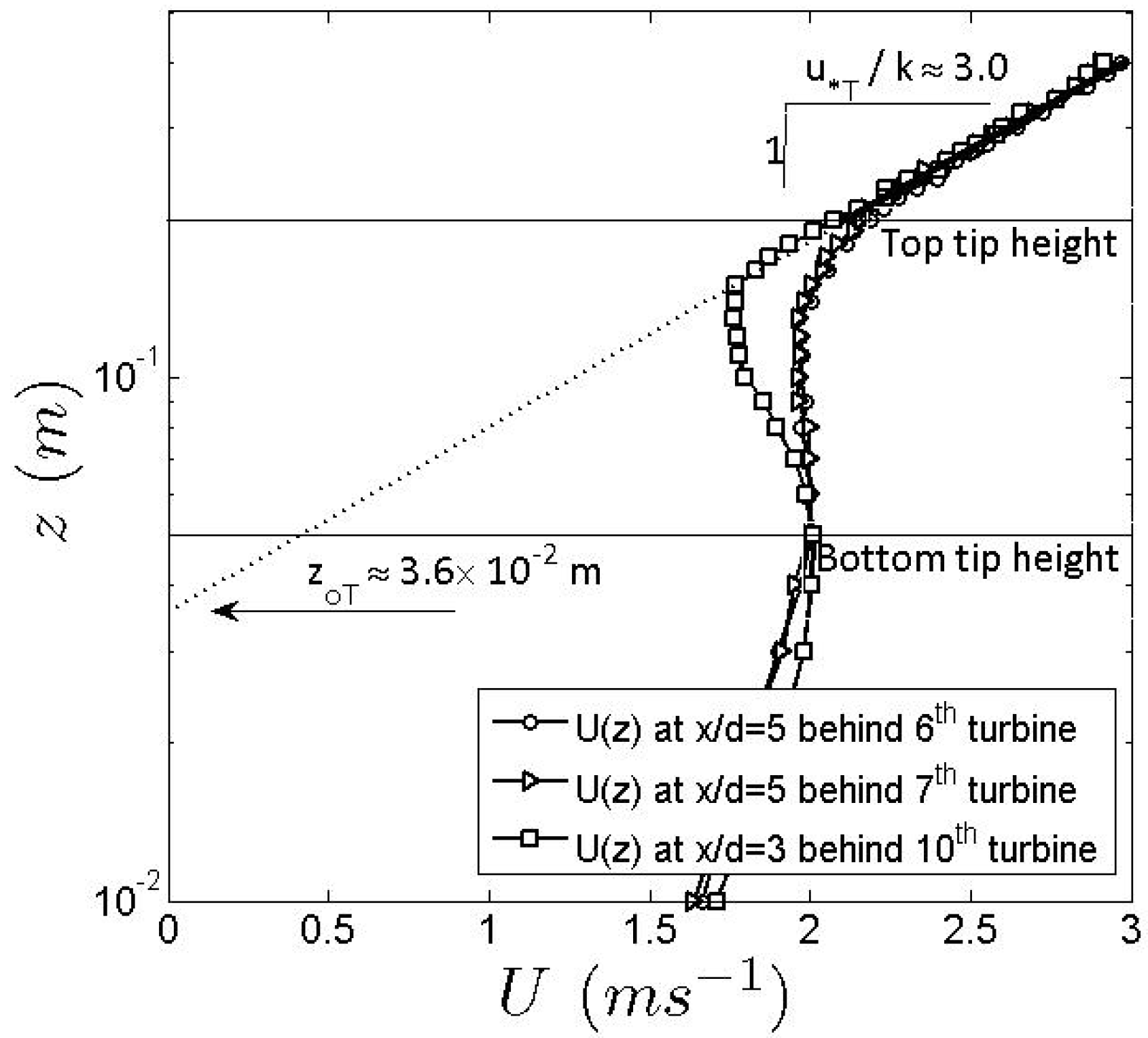
In this experiment, the characteristic surface roughness of the model wind farm was obtained from the adjusted logarithmic region, i.e., starting from the sixth row of wind turbines. A schematic of the calculation is shown in Figure 14. There, a value of $z_0$ = 3.6 × 10${}^{-2}$ m was found for the case $S_x$ = 5, which is roughly four times higher than that predicted by Equations (7) and (8). The departure between the measured and predicted value of the wind farm roughness highlights the intrinsic difficulties of its parameterization. It should also be noted that one factor that could contribute to the overestimation of the wind farm roughness is the fact that it is based on measurements collected only at the center plane (y = 0). Recent large-eddy simulations of the same flow have shown that, for that wind farm configuration, including spanwise variability leads to smaller roughness estimates [35]. Future research will address this issue using both LES and additional wind-tunnel experiments.

Figure 14. Aerodynamic roughness length of the wind farm array for the case $S_x$ = 5.

Figure 14. Aerodynamic roughness length of the wind farm array for the case $S_x$ = 5.

4. Summary

Wind tunnel experiments were performed to study the flow characteristics inside and above a model wind farm composed of 10 by 3 miniature wind turbines placed in a boundary layer flow. Two layouts of aligned wind turbines were considered in this study. They were characterized by inter-turbine separations of 5 and 7 rotor diameters in the streamwise direction by 4 rotor diameters in the spanwise direction. Cross-wire anemometry was used to obtain high resolution measurements of two velocity components (streamwise and vertical), turbulence intensity, and kinematic shear stress at different locations around the wind farm. Velocity spectra, turbulent energy production, and pdf were also calculated at various locations to better understand the structure of the turbulent flow.

Overall results suggest that the turbulent flow can be characterized by two broad regions. The first is located below top tip height of the wind turbines and it has a direct effect on the performance of the turbines. In that region, turbulence statistics appear to reach equilibrium as close as the third to fourth row of wind turbines. In the second region, located directly above the first, flow statistics adjust slowly. In this region, two distinctive layers were found: an internal boundary layer and an equilibrium layer. In the former, both the incoming flow and the wind turbines modulate the turbulence characteristics of the flow, while in the latter, flow statistics are conditioned mainly by the wind farm. The clear presence of these two layers allows, from a large-scale perspective, the treatment of large wind farms as a special case of surface roughness transition. In that characterization, the specification of the representative roughness length and the friction velocity associated with the wind farm is required. The determination of these parameters is not trivial. Indeed, the standard approach for their estimation is through the use of the log-law, which is strictly only valid under homogeneous conditions. Our results show that a well-defined logarithmic velocity profile is reached only after the sixth-seventh row of wind turbines. Upwind of this location, and similar to the case of a surface roughness transition, the flow is still adjusting and the determination of those parameters is more complicated. In this experiment, the representative surface roughness length, obtained in the fully adjusted log region, was found to be greater than predicted by standard formulations.

Similar to the situation of the wake of a single wind turbine in a boundary layer flow, the mean velocity distribution inside the farm is not axisymmetric, although the mean velocity deficit ($\Delta U_x=U-U_{incoming}$) has a roughly symmetric structure between the bottom and top tip heights. This property allows, in principle, to generalize parameterizations of the mean velocity inside wind farms, while accounting for the effects of the incoming boundary layer flow.

Turbulence intensity in region I of the wind farm shows a non-symmetric structure with respect to the turbine axis. Like the case of a single wind turbine ([25,34]), the non-uniformity of the boundary-layer flow is responsible for this effect. A strong enhancement of the turbulence levels around the top tip level was observed with respect to the turbulence generated behind a single wind turbine. The enhancement of the turbulence intensity appears to reach its highest levels behind the fourth turbine. This result contradicts some formulations that assume a monotonic increase of the turbulence levels with downwind distance in the farm. The peak of the velocity fluctuations is localized between one and three rotor diameters behind each turbine.

Power spectra of the streamwise and vertical velocity components show the signature of helicoidal tip vortices on the turbulence structure in the wind farm for an inter-turbine separation of seven rotor diameters ($S_x$ = 7). On the other hand, the higher levels of turbulence present in the case of $S_x$ = 5 preclude a noticeable signature of the tip vortices on the spectrum inside the farm. This is consistent with the stronger signature of the helicoidal tip vortices observed behind the first wind turbine, where the background turbulence is relatively low. In general, the velocity spectrum of the vertical velocity component shows a stronger signature of the tip vortices, compared with the streamwise velocity counterpart.

Future work will include the effect of thermal stratification—with different wind-turbine layouts—on the structure of the turbulent flow inside and above wind farms. Also a comprehensive analysis of the surface roughness estimation will be performed including different turbine layouts (streamwise spacing with aligned turbines, staggered configurations and irregular randomly spaced turbines). The datasets obtained from these experiments will also be used for validation of numerical simulation codes (e.g., LES) as recently done by Wu and Porté-Agel [34] and Porté-Agel et al. [35] for the single turbine case.