Unbalanced Magnetic Pull Calculation in Ironless Axial Flux Motors

Abstract

Axial flux motors have gained widespread attention in the field of electric vehicles. The stator may exert a unilateral axial force on the dual rotors under uneven air gaps. The unbalanced magnetic pull can influence the production and processing of the motor, leading to issues such as vibrations, bearing degradation, reduced lifespan, and torque reduction attributed to the bearings. Accurate evaluation of the unilateral magnetic pull can reduce costs associated with bearing protection. For dual-rotor motors, the axial forces of the rotors act in opposite directions with nearly equal magnitudes, resulting in the catastrophic cancellation of unbalanced magnetic pull calculations. A similar phenomenon may occur between coils, introducing computational errors. To avoid these errors, the stator was selected as the computational target for unilateral axial force calculations. The integration domain was defined to encompass the entire air region containing all windings, rather than summing individual force components. This merged integration approach was mathematically validated through the Maxwell stress tensor method. Finally, the obtained stator axial force closely matched the rotor axial force in magnitude, demonstrating the accuracy of the proposed method.

1. Introduction

Axial flux motors offer a significant benefit in terms of torque density, making them particularly advantageous in scenarios where space and weight constraints, especially in axial length, are critical. This has led to their increasing popularity in the electric vehicle sector [1,2,3]. In order to topologically avoid unbalanced magnetic pull, axial flux motors usually have double-sided air gaps, that is, either a two-rotor, single-stator configuration or a two-stator, single-rotor configuration. However, when the machining accuracy is not ideal, the rotors of the axial flux motor with a double air gap will produce an axial force and exert it on the bearing, affecting the life of the bearing [4,5,6]. Accurate evaluation of the unilateral magnetic pull can reduce costs associated with bearing protection.

Axial flux motors usually include coils, permanent magnets, rotor yokes, and the motor shaft, as shown in Figure 1. The rotors are held together by the motor shaft, as shown in Figure 2. When the production of the motor causes the air gaps on both sides to be unequal, the axial forces on the two rotors are not the same, resulting in an unbalanced magnetic pull on the motor shaft.

The causes of unilateral magnetic pull include non-uniform rotor magnetization [7], winding short circuits [8], magnetic saturation [9], and air-gap non-uniformity. The unilateral magnetic pull caused by non-uniform air gaps is primarily studied in radial flux motors. Rui Zhu [10] and colleagues investigated the unilateral magnetic pull in radial inner-rotor motors under circumferential air-gap non-uniformity. Their study analyzed the following three scenarios: static eccentricity, dynamic eccentricity, and compound eccentricity (a combination of static and dynamic eccentricities). Rafal Piotr Jastrzebski [11] et al. investigated the unilateral magnetic pull caused by circumferential eccentricity in active bearing control systems. Yang Zhou [12] et al. used the finite element method to calculate the unilateral magnetic pull of a squirrel-cage induction motor with an uneven air gap. David G. Dorrell et al. [13]. established an analytical model for squirrel-cage induction motors to study the damping phenomenon of unilateral magnetic pull caused by rotor dynamic eccentricity.

The incorporation of complex geometries and nonlinearities arising from ferromagnetic materials in motor models necessitates the adoption of numerical computation as an established methodology for analyzing unilateral magnetic pull (UMP). Jiwen Zhang et al. conducted a comprehensive finite element analysis (FEA) of unilateral magnetic pull (UMP) in a 1000 MW hydro-generator system, underscoring the criticality of assembly tolerances in electromagnetic alignment [14]. X. Wen et al. leveraged commercial finite element software to compute magnetic field distributions, subsequently conducting a systematic investigation into the impact of the pole-slot configuration on unilateral magnetic pull (UMP) through parametric simulations [15]. Yongxing Song et al. conducted computational investigations of unilateral magnetic pull (UMP) induced by non-uniform loading through finite element analysis (FEA) tools, achieving a quantitative assessment of electromagnetic-structural coupling effects under asymmetric operating conditions [16].

Research on unilateral magnetic pull in axial flux motors is relatively limited. Xiaoting Zhang et al. [17]. established an analytical model for a dual-outer-rotor motor with a central rotor to address the unilateral magnetic pull caused by eccentricity. Seyyed Mehdi Mirimani et al. [18]. used finite element analysis to calculate the unilateral magnetic pull in a single stator-single rotor axial flux motor under inclined eccentricity conditions. Some researchers have conducted studies on eccentricity detection, but did not address the calculation of unilateral magnetic pull [19,20,21].

The calculation of unilateral magnetic pull varies for motors with different topological structures. For dual-rotor motors, the axial forces of the rotors act in opposite directions with nearly equal magnitudes, resulting in the catastrophic cancellation of unbalanced magnetic pull calculations. This phenomenon occurs when using numerical calculation methods such as the finite element method. Therefore, it is essential to select an appropriate calculation method.

The ideal approach is to use numerical calculations to derive a single resultant force only. It is an appropriate choice to calculate the stator axial force to represent the unilateral magnetic pull. According to the Maxwell stress tensor method, the calculation of the stator axial force can be converted into a surface integral over the air domain enclosing all the coils [22,23]. This conclusion can be proved by numerical calculation [24,25,26,27], since the most classical method to derive the tensor involves using the Gauss flux theorem to obtain the tensor on the closed surface [28,29,30,31]. This conclusion has been widely used in the calculation of magnetic force and electromagnetic torque [32,33,34,35].

The main innovation of this paper lies in being the first to identify the catastrophic cancellation caused by large-number subtraction during unilateral magnetic pull calculations in dual outer-rotor axial flux motors, and proposing a novel air-region substitution method surrounding the stator (instead of rotor components) to resolve this computational instability in axial force determinations. The main contributions of this paper are as follows: Section 2 demonstrates the errors in unilateral magnetic pull (UMP) calculations caused by the force superposition method. Section 3 determines the integration region of the Maxwell stress tensor and discusses its merging process. Section 4 calculates the UMP of the motor at full load, with the accuracy of the proposed method being validated through comparative analysis of stator and rotor axial forces. The appendix provides a similar calculation case to verify the effectiveness of the proposed method.

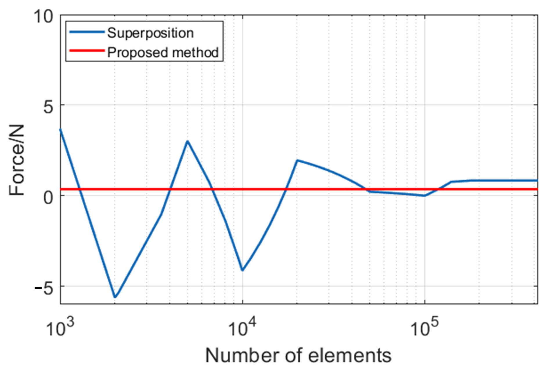
2. Catastrophic Cancellation

To obtain an accurate unilateral magnetic pull, it is necessary to avoid errors caused by “catastrophic cancellation” in numerical calculations. In axial flux motors, the two rotor discs exhibit significant mutual attraction, resulting in opposing axial force components with large magnitudes. The algebraic sum of these two forces (i.e., the unilateral magnetic pull) is highly sensitive to calculation errors in either component.

For instance, we have the following:

True axial forces: 100 N and −99 N ⇒ Actual unilateral pull: 1 N.

With 1% calculation errors: 101 N and −98 N ⇒ Calculated pull: 3 N.

Error magnitude: 200%,

This demonstrates how small relative errors in large opposing forces can lead to catastrophic errors in the net force calculation. This issue may lead to significant calculation errors in the unilateral magnetic pull.

As shown in Figure 3, this is an ironless axial flux motor, which includes coils, main permanent magnets, and auxiliary permanent magnets. The main permanent magnets (PMs) generate axial flux, while the auxiliary PMs generate tangential flux to increase air gap flux and reduce rotor yoke leakage. The axial magnetic field turns tangential at the rotor yokes on both sides, forming a complete magnetic circuit. Under the axial magnetic field, the effective sections of the coils generate tangential forces, which result in torque.

The design requirements of the motor are listed in

Table 1. Design requirements.

Attribute	Parameter
Maximum torque/Nm	500
Maximum speed/rpm	2000
Number of phase	3
Outer radius of PM/mm	120
Inner radius of PM/mm	64

. And the main parameters are shown in

Table 2. Main parameters.

Attribute	Parameter
Rotor topology	Double outer rotor NS topology
Permanent magnet	N48H
Slot-pole combination	10-pole-12-slot
Phase current amplitude/A	720
Turns of coil	24
Air gap thickness/mm	1.75
Axial thickness of coil/mm	24
Main PM thickness/mm	16
Auxiliary PM thickness/mm	16
Main PM pole-arc coefficient	0.75
Rotor yoke thickness/mm	3
Stator axial offset/mm	+0.5

. The double outer rotor NS topology is used to increase torque. For selecting the slot-pole combination, common choices for fractional-slot concentrated windings include 8-pole 9-slot, 10-pole 12-slot, and 8-pole 12-slot configurations.

Based on the winding factor and the suppression of harmonics of the electromagnetic force, the chosen slot-pole combination is 10-pole-12-slot. For the phase current amplitude, a value of 720 A achieves the torque goal listed in Table 1. All axial force computations presented in this study have been obtained under the specified current conditions. Given the inner and outer radii of the PMs, the number of coil turns is set at 24, using 1 mm thick copper wire arranged in two layers. The thickness of the main PMs and the axial thickness of the coils are designed to maximize torque density. The main PM pole-arc coefficient is designed to achieve maximum torque. The rotor yoke thickness is designed with reference to [36].

The principle of virtual work is a widely used method for calculating electromagnetic forces. Its general computational approach involves taking the derivative of electromagnetic energy $W_e$ with respect to displacement x:

$$\mathit{F}=-{\displaystyle \frac{\partial W_e}{\partial x}}$$

(1)

Alternatively, it can be derived through the equilibrium equation:

$$\int {\mathcal{T}}_{virtual}·\delta \mathit{A}dS=\int {\mathcal{T}}_{MST}:\delta ϵdV-\int \mathit{J}·\delta \mathit{A}dV$$

(2)

where ${\mathcal{T}}_{virtual}$ is the sought force density tensor and $\delta \mathit{A}$ represents the virtual displacement. ${\mathcal{T}}_{MST}$ is the Maxwell stress tensor, and $\delta ϵ$ is the virtual strain tensor derived from the virtual displacement. $\mathit{J}$ is the current density.

The stator axial force calculated using the virtual principle and the total axial force of the two rotors are illustrated in Figure 4. The axial force is calculated over one electrical cycle. The blue curve corresponds to the total axial force of the stator, averaging 170 N, while the red curve represents the combined axial force of the two rotors, with an average value of 299 N. The difference between the two calculations is significant, approaching nearly 50%. The inconsistency between the rotor axial force and stator axial force violates mechanical laws, rendering the current computational results unreliable.

As shown in Figure 5, the calculated axial forces for two rotors are presented. The blue curve corresponds to the upper rotor’s axial force with an average value of −2176 N, while the red curve represents the lower rotor’s axial force, averaging 1877 N. The axial forces on both sides of the rotor are in opposite directions. The axial force variation caused by air gap non-uniformity is minimal; therefore, calculating unilateral magnetic pull using only the rotor results in inaccuracies.

However, computational inaccuracies in rotor analysis do not validate the stator’s results. As shown in Figure 6, the axial forces between a Phase A coil and a Phase C coil are illustrated. The blue curve corresponds to the Phase A coil’s axial force with an average value of 5.3 N, while the red curve represents the Phase C coil’s axial force, averaging −3.7 N. Similar calculation errors have also been identified in the stator.

Ideal verification for unilateral magnetic pull simulation should involve comparable electromagnetic force calculations from both rotor and stator sides. However, unexpected errors have been identified in the calculation of both stator and rotor axial forces. Therefore, a viable approach is to adopt force calculation methods that merge rotor force calculation zones, directly deriving the net force rather than summing individual electromagnetic forces from each permanent magnet.

The Maxwell stress tensor method can circumvent this issue. With this approach, the unilateral magnetic pull can be derived through the integration of the magnetic flux density B within a single calculation zone. Notably, the magnetic flux density is obtained by solving differential equations using non-superposition methods rather than superpositionbased approaches. Therefore, these errors can be effectively eliminated by adopting this calculation method.

3. Theoretical Derivation

3.1. Maxwell Stress Tensor

Before deducing the expression of the Maxwell stress tensor, it is necessary to determine whether magnetization current, polarization charge, polarization current, surface charge, and surface current contribute to the total electromagnetic force.

Suppose there is a region of ferromagnetic material and a free current. According to the Lorentz formula, the force density of a free current in a magnetic field is as follows:

$$\mathit{f}={\mathit{J}}_f\times \mathit{B}$$

(3)

According to Maxwell’s equations, we can obtain the following:

$$\nabla \times \mathit{H}={\mathit{J}}_f+{\displaystyle \frac{\partial \mathit{D}}{\partial t}}$$

(4)

Substituting Equation (4) into Equation (3), we can obtain the following:

$$\mathit{f}=(\nabla \times \mathit{H})\times \mathit{B}-{\displaystyle \frac{\partial \mathit{D}}{\partial t}}\times \mathit{B}$$

(5)

$$\begin{array}{cc}\hfill \mathit{f}=& [\nabla \times ({\displaystyle \frac{\mathit{B}}{{\mu }_0}}-\mathit{M})]\times \mathit{B}-\left[{\displaystyle \frac{\partial }{\partial t}}({ϵ}_0\mathit{E}+\mathit{P})\right]\times \mathit{B}\hfill \\ \hfill =& {\displaystyle \frac{1}{{\mu }_0}}(\nabla \times \mathit{B})\times \mathit{B}-(\nabla \times \mathit{M})\times \mathit{B}\hfill \\ \hfill & -{\displaystyle \frac{\partial \mathit{P}}{\partial t}}\times \mathit{B}-{ϵ}_0{\displaystyle \frac{\partial \mathit{E}}{\partial t}}\times \mathit{B}\hfill \\ \hfill =& {\displaystyle \frac{1}{{\mu }_0}}(\nabla \times \mathit{B})\times \mathit{B}-{\mathit{J}}_M\times \mathit{B}-{\mathit{J}}_P\times \mathit{B}-{\mathit{J}}_D\times \mathit{B}\hfill \end{array}$$

(6)

where ${\mathit{J}}_P$ and ${\mathit{J}}_D$ represent the equivalent polarization current and displacement current, respectively.

To comprehend Equation (6), we can apply the idea of reluctance force as discussed in References [28,37]. If there is only one permanent magnet and one piece of iron in space, and they remain relatively static, this means that there is no free current, polarization current, or displacement current. The obvious conclusion is that there is a magnetic force between the two. According to Equation (3), the magnetic force, as calculated by Equation (6), is zero, which is inconsistent with reality. Therefore, in the derivation of this paper, the role of the magnetization current is taken into account, and its mathematical expression is ${\mathit{J}}_M\times \mathit{B}$, which appears in Equation (6). Polarization currents can be handled in the same way, that is, ${\mathit{J}}_P\times \mathit{B}$. It is worth mentioning that the negative sign of the equivalent magnetization current term and the equivalent polarization current term means that the action of these two currents is not considered, while the negative sign of the displacement current term means that its contribution should be subtracted. In fact, the contribution of the displacement current is reflected in the electric component of the Maxwell stress tensor through electromagnetic induction.

In the same way, we can obtain the following:

$$\begin{array}{cc}\hfill \mathit{f}& =[\nabla ·({ϵ}_0\mathit{E}+\mathit{P})]\mathit{E}\hfill \\ \hfill & ={ϵ}_0(\nabla ·\mathit{E})\mathit{E}+(\nabla ·\mathit{P})\mathit{E}\hfill \\ \hfill & ={ϵ}_0(\nabla ·\mathit{E})\mathit{E}-{\rho }_P\mathit{E}\hfill \end{array}$$

(7)

where ${\rho }_P$ is the equivalent polarization charge.

Similar to the treatment of magnetizing current, the contribution of the polarization charge is ${\rho }_P\mathit{E}$.

We should also consider whether the equivalent magnetization current and equivalent polarization current can exist as surface currents. The reasons for the contribution of the equivalent magnetization current and equivalent polarization current to the force have been elucidated. Then the boundary value relationship between the medium and vacuum interface needs to be reconsidered. The contribution of the medium to the magnetic field will be represented by the current, not the permeability or magnetization.

As shown in Figure 7, assuming that there is a smooth interface between a medium and a vacuum, and there is no free current in the region. The magnetic induction intensity $\mathit{B}$ will change when it passes through the interface. A counterclockwise loop with a length of $l_1$ and a width of $l_2$ is taken in the neighborhood of the mutation point. The magnetic induction intensity on the medium side is ${\mathit{B}}_{-}$, and that on the vacuum side is ${\mathit{B}}_{+}$. ${\mathit{e}}_n$ is the unit normal vector pointing from the medium to the vacuum. When the rectangular loop is small enough, the magnetic induction intensity $\mathit{B}$ on the same side can be considered uniform. At this point, the Ampere circuital theorem can be expressed as follows:

$${\displaystyle \frac{1}{{\mu }_0}}\underset{\partial A}{\mathit{\oint }}\mathit{B}·d\mathit{l}=\underset{A}{\mathit{\int }}({\mathit{J}}_f+{\mathit{J}}_M+{\mathit{J}}_P+{\mathit{J}}_D)·d\mathit{S}$$

(8)

where A is a surface and $\partial A$ is its closed boundary. Using the Ampere circuital theorem for the rectangular circuit, the relationship between magnetization current and polarization current, and magnetic induction intensity inside and outside the interface can be obtained:

$${\mathit{e}}_n\times ({\mathit{B}}_{+}-{\mathit{B}}_{-})={\mu }_0({\mathit{K}}_M+{\mathit{K}}_P+{\mathit{K}}_D)$$

(9)

where $B_{t+}$ and $B_{t-}$ are tangential components of magnetic induction intensity inside and outside the interface, respectively. $K_M$, $K_P$, and $K_D$ are the current densities of magnetization current, polarization current, and displacement current, respectively.

Equation (9) shows that the boundary conditions on the interface will be represented by their surface currents when the contributions of magnetization currents, polarization currents, and displacement currents to the forces are acknowledged, which means that for equivalent magnetization currents, polarization currents, and displacement currents, it is necessary to consider their effects as volume currents and surface currents at the same time.

For the free current in a conductor, the current distribution affects the calculation of the total force. The existence of the Hall effect means that the current distribution changes under the action of an external magnetic field, leading to the appearance of surface current. The Hall effect shows that when the free current is perpendicular to the uniform magnetic field, the free charge is deflected by the Lorentz force, generating electric fields perpendicular to the direction of the current and magnetic field. When the electric field force is equal to the Lorentz force, the electric field tends to be stable and produces a fixed potential difference. The intensity of the electric field is proportional to the average velocity of the free charge.

Assuming that the average velocity of free charge per unit volume is the same after equilibrium, the Hall effect produces a uniform electric field in the conductor. When a random cylinder is placed within the conductor, aligned with the direction of the electric field, the Gauss flux theorem applies. Since the electric field remains constant, the overall charge within the cylinder amounts to zero. This means there is no build-up of charge inside the conductor. In fact, the free charge deflected by the Lorentz force is not stationary, but is attached to the conductor surface and moves directionally under the action of the electromotive force of the power source, forming a surface current. Therefore, in the calculation of the total force, the existence of free currents as surface currents is not negligible. Therefore, Equation (9) can be rewritten as follows:

$${\mathit{e}}_n\times ({\mathit{B}}_{+}-{\mathit{B}}_{-})={\mu }_0({\mathit{K}}_f+{\mathit{K}}_M+{\mathit{K}}_P+{\mathit{K}}_D)$$

(10)

where $K_f$ is the free current. The displacement current term is usually considered meaningless because it should approach zero. However, in this paper, it is considered that the displacement current term represents the mutual transformation of electric fields and magnetic fields, so the displacement current is also expressed as the surface current:

$${\mathit{K}}_D=o{ϵ}_0{\displaystyle \frac{\partial {\mathit{E}}_e}{\partial t}}$$

(11)

where o is an infinitesimal in meters and ${\mathit{E}}_e$ is the external electric field.

For free charges, it is generally accepted that they can exist as surface charges. Therefore, we can discuss both free charge and polarization charge at the same time. Then the boundary conditions on the interface between the medium and the vacuum need to be reconsidered. The contribution of the medium to the electric field will be represented by the charge, not by the dielectric constant or the intensity of the polarization.

As shown in Figure 8, it is assumed that there is a medium within a spatial domain $\mathsf{\Omega }$, and the dielectric constant is ${ϵ}_{-}$. There is a smooth interface between the medium and the outside world. The external dielectric constant is ${ϵ}_{+}$. Then the electric field intensity $\mathit{E}$ will change when it passes through the interface. A cylindrical region with a radius of r and a height of h is taken in the neighborhood of the abrupt change point. The electric field intensity on the side of the medium is ${\mathit{E}}_{-}$, and the electric field intensity on the outside is ${\mathit{E}}_{+}$. ${\mathit{e}}_n$ is the unit normal vector pointing from the medium to the outside. When the cylindrical region is small enough, the electric field intensity $\mathit{E}$ on the same side can be considered uniform. At this point, the Gauss flux theorem can be expressed as follows:

$${ϵ}_0\underset{\partial \mathsf{\Omega }}{\oint }\mathit{E}·d\mathit{S}=\underset{\mathsf{\Omega }}{\int }({\rho }_f+{\rho }_P)dV$$

(12)

where ${\rho }_f$ and ${\rho }_P$ are the charge densities of free charges, respectively.

Using the Gauss flux theorem for the cylindrical region, the following equation can be obtained:

$${\mathit{e}}_n·({\mathit{E}}_{+}-{\mathit{E}}_{-})={\displaystyle \frac{1}{{ϵ}_0}}({\sigma }_f+{\sigma }_P)$$

(13)

where $E_{n-}$ and $E_{n+}$ are the normal components of the electric field intensity on the inner and outer surfaces of the interface, respectively.

Equation (13) shows that the boundary conditions on the interface will be represented by their surface charges if the contributions of free and polarization charges to the force are admitted. This means that for both free and polarization charges, it is necessary to consider their effects as both volume charges and surface charges.

As shown in Figure 9, a counterclockwise loop with length $l_1$ and width $l_2$ is taken in the neighborhood of the mutation point on the interface. The electric field intensity on the side of the medium is ${\mathit{E}}_{-}$ and the electric field intensity on the outside is ${\mathit{E}}_{+}$. ${\mathit{e}}_n$ is the unit normal vector pointing outward from the medium. When the rectangular loop is small enough, the electric field intensity $\mathit{E}$ on the same side can be considered uniform. According to Faraday’s law of electromagnetic induction, we have the following:

$$\underset{\partial A}{\mathit{\oint }}\mathit{E}·d\mathit{l}=-{\displaystyle \frac{\partial }{\partial t}}\underset{A}{\mathit{\int }}\mathit{B}·d\mathit{S}$$

(14)

where A is the integral surface and $\partial A$ is the curvilinear closed boundary.

Using the electromagnetic induction law for the rectangular circuit, we can obtain the following:

$${\mathit{e}}_n\times ({\mathit{E}}_{+}-{\mathit{E}}_{-})=-{\displaystyle \frac{1}{2}}o{\displaystyle \frac{\partial }{\partial t}}({\mathit{B}}_{+}+{\mathit{B}}_{-})$$

(15)

where $E_{-}$ and $E_{+}$ are the electric field intensities on the inner and outer surfaces of the interface. $B_{-}$ and $B_{+}$ are the magnetic induction intensities on the inner and outer surfaces of the interface. o is an infinitesimal quantity measured in meters.

Through the above analysis, it can be concluded that the equivalent magnetization current, equivalent polarization current, and equivalent polarization charge can contribute to the electromagnetic force. According to Equations (7) and (6), the equivalent magnetization current, equivalent polarization current, and equivalent polarization charge can be directly calculated as free current and free charge using the Lorentz formula. Therefore, there should be a unified procedure for deriving the expression of the Maxwell stress tensor, which can take into account free current, free charge, polarization of the medium, and magnetization of the medium simultaneously. In this paper, the calculation of Lorentz forces is considered in two cases: surface integrals and volume integrals. The latter can be evaluated using suitable Gaussian surfaces as per the Gauss flux theorem, while the former cannot.

Considering that charges and currents cannot exert forces on themselves, the surface density of forces on surface currents and charges in the electromagnetic field can be expressed as follows:

$${\mathit{f}}_S=({\sigma }_f+{\sigma }_P){\mathit{E}}_e+({\mathit{K}}_f+{\mathit{K}}_P+{\mathit{K}}_M)\times {\mathit{B}}_e$$

(16)

where ${\mathit{E}}_e$ and ${\mathit{B}}_e$ are the external electric field and the external magnetic field at the surface element, respectively.

The electric and magnetic fields at the surface element can be considered as the superposition of the fields generated by the surface element itself and the external electric and magnetic fields. Considering that the electric field and magnetic field generated by the source at the surface element, inside and outside the interface, are in opposite directions and equal in magnitude, the electric field intensity and magnetic induction intensity inside and outside the interface can be expressed as follows:

$$\begin{array}{cc}\hfill {\mathit{E}}_{+}& ={\mathit{E}}_e+{\mathit{E}}_s\hfill \\ \hfill {\mathit{E}}_{-}& ={\mathit{E}}_e-{\mathit{E}}_s\hfill \end{array}$$

(17)

$$\begin{array}{cc}\hfill {\mathit{B}}_{+}& ={\mathit{B}}_e+{\mathit{B}}_s\hfill \\ \hfill {\mathit{B}}_{-}& ={\mathit{B}}_e-{\mathit{B}}_s\hfill \end{array}$$

(18)

where ${\mathit{E}}_s$ and ${\mathit{B}}_s$ are the electric field intensity and magnetic induction intensity generated by the surface element, respectively.

Expressions of the external electric field and magnetic field can be obtained from the following: Equations (17) and (18):

$$\begin{array}{cc}\hfill {\mathit{E}}_e& ={\displaystyle \frac{1}{2}}({\mathit{E}}_{+}+{\mathit{E}}_{-})\hfill \\ \hfill {\mathit{B}}_e& ={\displaystyle \frac{1}{2}}({\mathit{B}}_{+}+{\mathit{B}}_{-})\hfill \end{array}$$

(19)

Substituting Equations (10), (13) and (19) into Equation (16), we can obtain the following:

$$\begin{array}{cc}\hfill {\mathit{f}}_S=& {\displaystyle \frac{1}{2}}{ϵ}_0[{\mathit{e}}_n·({\mathit{E}}_{+}-{\mathit{E}}_{-})]({\mathit{E}}_{+}+{\mathit{E}}_{-})\hfill \\ \hfill & +{\displaystyle \frac{1}{2{\mu }_0}}[{\mathit{e}}_n\times ({\mathit{B}}_{+}-{\mathit{B}}_{-})]\times ({\mathit{B}}_{+}+{\mathit{B}}_{-})\hfill \\ \hfill & -{\displaystyle \frac{1}{2}}{\mathit{K}}_D\times ({\mathit{B}}_{+}+{\mathit{B}}_{-})\hfill \\ \hfill =& {\displaystyle \frac{1}{2}}{ϵ}_0[{\mathit{e}}_n·({\mathit{E}}_{+}-{\mathit{E}}_{-})]({\mathit{E}}_{+}+{\mathit{E}}_{-})\hfill \\ \hfill & +{\displaystyle \frac{1}{2{\mu }_0}}[({\mathit{B}}_{+}+{\mathit{B}}_{-})·{\mathit{e}}_n]({\mathit{B}}_{+}-{\mathit{B}}_{-})\hfill \\ \hfill & -{\displaystyle \frac{1}{2{\mu }_0}}[({\mathit{B}}_{+}+{\mathit{B}}_{-})·({\mathit{B}}_{+}-{\mathit{B}}_{-})]{\mathit{e}}_n\hfill \\ \hfill & -{\displaystyle \frac{1}{2}}{\mathit{K}}_D\times ({\mathit{B}}_{+}+{\mathit{B}}_{-})\hfill \end{array}$$

(20)

The surface density of the force contributed by the surface current and the surface charge in the electromagnetic field can be expressed as a tensor ${\mathcal{T}}_S$:

$${\mathit{f}}_S={\mathcal{T}}_S·{\mathit{e}}_n$$

(21)

$$\begin{array}{cc}\hfill T_{Sij}=& {ϵ}_0(E_{i+}{E}_{j+}-E_{i-}{E}_{j-}-{\displaystyle \frac{1}{2}}{\delta }_{ij}{E}_{+}^2+{\displaystyle \frac{1}{2}}{\delta }_{ij}{E}_{-}^2)\hfill \\ \hfill & +{\displaystyle \frac{1}{{\mu }_0}}(B_{i+}{B}_{j+}-B_{i-}{B}_{j-}-{\displaystyle \frac{1}{2}}{\delta }_{ij}{B}_{+}^2+{\displaystyle \frac{1}{2}}{\delta }_{ij}{B}_{-}^2)\hfill \end{array}$$

(22)

Considering the effects of polarization charge, magnetization current, and polarization current in Equations (6) and (7), the force density of the volume current and volume charge in the electromagnetic field is as follows:

$${\mathit{f}}_V=({\rho }_f+{\rho }_P){\mathit{E}}_e+({\mathit{J}}_f+{\mathit{J}}_M+{\mathit{J}}_P)\times {\mathit{B}}_e$$

(23)

where ${\rho }_f$, ${\rho }_P$, ${\mathit{J}}_f$, ${\mathit{J}}_M$, and ${\mathit{J}}_P$ are the free charge, polarization charge, free current, magnetization current, and polarization current, respectively. ${\mathit{E}}_e$ and ${\mathit{B}}_e$ represent the external electric field and magnetic field, respectively. Similar to other derivations, we can obtain the force density corresponding to the volume current and the volume charge:

$${\mathit{f}}_V=\nabla ·{\mathcal{T}}_V-{ϵ}_0{\mu }_0{\displaystyle \frac{\partial {\mathit{S}}_{-}}{\partial t}}$$

(24)

$$T_{Vij}={ϵ}_0(E_{i-}{E}_{j-}-{\displaystyle \frac{1}{2}}{\delta }_{ij}{E}_{-}^2)+{\displaystyle \frac{1}{{\mu }_0}}(B_{i-}{B}_{j-}-{\displaystyle \frac{1}{2}}{\delta }_{ij}{B}_{-}^2)$$

(25)

$${ϵ}_0{\mu }_0{\displaystyle \frac{\partial {\mathit{S}}_{-}}{\partial t}}={ϵ}_0{\displaystyle \frac{\partial }{\partial t}}({\mathit{E}}_{-}\times {\mathit{B}}_{-})$$

(26)

The expression of the total force can be obtained from Equations (21) and (24):

$$\begin{array}{cc}\hfill \mathit{F}& =\underset{\mathsf{\Omega }}{\mathit{\int }}{\mathit{f}}_{V}dV+\underset{\partial \mathsf{\Omega }}{\mathit{\oint }}{\mathit{f}}_{S}dS\hfill \\ \hfill & =\underset{\partial \mathsf{\Omega }}{\mathit{\oint }}{\mathcal{T}}_t·d\mathit{S}-{ϵ}_0{\mu }_0{\displaystyle \frac{\partial }{\partial t}}\underset{\mathsf{\Omega }}{\mathit{\int }}{\mathit{S}}_{-}dV\hfill \end{array}$$

(27)

where ${\mathcal{T}}_t$ is the total Maxwell stress tensor and can be expressed as follows:

$$T_{tij}={ϵ}_0(E_{i+}{E}_{j+}-{\displaystyle \frac{1}{2}}{\delta }_{ij}{E}_{+}^2)+{\displaystyle \frac{1}{{\mu }_0}}(B_{i+}{B}_{j+}-{\displaystyle \frac{1}{2}}{\delta }_{ij}{B}_{+}^2)$$

(28)

According to Equation (28), the total Maxwell stress tensor is the classical Maxwell stress tensor. In calculating the total force, the integral region can be the outer surface of the interface. Equation (24) shows that the Maxwell stress tensor for any closed region is the classical Maxwell stress tensor.

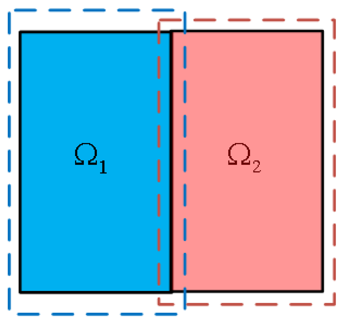
3.2. Determination and Merging of Integral Regions

This part justifies establishing the integration boundary at the interface’s exterior surface domain, particularly focusing on the vanishingly thin transitional layer enveloping the object at material discontinuities. This is because the magnetic induction intensity B will change abruptly when passing through the interface, resulting in different tangential components of the inner and outer surfaces of the interface. According to the above derivation, the total force of the medium in the electromagnetic field can be obtained by the integral of the volume density and surface density of the Lorentz force. So the total force of the medium in the region can be obtained by the integral of the Maxwell stress tensor on the outer surface of the interface. For two objects of different materials with a contact surface, as shown in Figure 10, the regions should be the two dotted boxes rather than the box with the dashed line. And these lines represent the outer surface of the interface. The results of integration on both sides of the interface are different, which means that the integration regions on the interface cannot cancel out. In this case, the resultant force on the objects should be the sum of the two integrals, rather than the sum of the integrals over the separate surfaces. This means that the contributions of the surface current and surface charge at the contact surface need to be considered twice.

The calculation of contact forces also involves a special case, as shown in Figure 11. There are different materials in region ${\mathsf{\Omega }}_1$ and region ${\mathsf{\Omega }}_2$. Region ${\mathsf{\Omega }}_1$ is completely surrounded by region ${\mathsf{\Omega }}_2$. In this case, the force exerted by region ${\mathsf{\Omega }}_1$ in the electromagnetic field can be obtained by integrating the Maxwell stress tensor over the dotted line. Obviously, the resultant force cannot be obtained by integrating the Maxwell stress tensor on the dashed line. In this case, if the material of region ${\mathsf{\Omega }}_2$ is replaced by vacuum, the results still hold, meaning that the integral result of the Maxwell stress tensor method is not independent of the choice of integral path, even if the integral region is in vacuum and contains no charge or current. Thus, it can be concluded that the integral region for the Maxwell stress tensor method must be located on the outer surface of the object interface.

However, in the absence of surface magnetization currents, the magnetic field within can be considered uniform as long as the gap between the two objects is sufficiently small. For engineering calculations, the integration regions involved can be consolidated.

4. Calculation of Unbalanced Magnetic Pull

According to the above analysis, when using the Maxwell stress tensor method, the integration region should be located on the outer surface of the interface of each object. Integration domains may be consolidated when inter-object air gap dimensions fall below critical thresholds and the magnetization current is absent.

The establishment of a simulation model is imperative for validating the accuracy of force computations. As illustrated in Figure 12, this represents a single-stator single-rotor motor configuration. The unilateral retention of the rotor serves to precisely quantify the total axial force acting on the rotor assembly, enabling direct comparison with the stator’s axial force output to validate the computational methodology. The rotor yoke has been omitted for computational acceleration. Integration regions for both stator and rotor components are explicitly delineated in the schematic.

The magnitude of the average axial force obtained using various methodologies is illustrated in Figure 13. In the figure, blue data represent stator-derived axial forces, while red data correspond to rotor-generated axial forces. The superposition method employs the volume force density calculations for individual components, followed by axial force summation. The calculation method of volume force can be expressed as follows:

$${\mathit{F}}_{volume}=\sum _{i=0}^{i=N}{\mathcal{T}}_i·{\mathit{n}}_i{A}_i{V}_i$$

(29)

where ${\mathcal{T}}_i$ is the Maxwell stress tensor, $A_i$ is the area of side i of the element, ${\mathit{n}}_i$ is the normal vector of the corresponding face, $V_i$ is the volume of the element.

The proposed methodology yields axial forces of 76.7 N and 75.4 N in the diagram, compared to 238.2 N/100.8 N via the virtual work principle and 252.8 N/100.8 N using the superposition method. And the simulation results are 170.1 N and 76.6 N. Computational results demonstrate the proposed method’s superior accuracy, with closely aligned axial force values. Both the virtual work principle and superposition method exhibit significant errors (>64% deviation), although their stator-/rotor-specific results show internal consistency, suggesting that force superposition may dominate the virtual work principle’s error propagation. The dataset is comprehensively presented in

Table 3. Axial force data comparison.

Method	Stator	Rotor
Proposed method	76.7 N	75.4 N
Virtual work principle	238.2 N	100.8 N
Superposition method	252.8 N	100.8 N
Simulation	170.1 N	76.6 N

.

For a well-configured simulation model, the numerical solution generally remains stable under given parameters. However, it shows significant dependence on the number of grid cells/mesh density used in discretization. As shown in Figure 14, the relationship between axial force and grid density (number of elements) is illustrated. The horizontal axis represents the total number of elements of the stator and rotor, while the vertical axis denotes the axial force. The blue curve corresponds to stator data, the red solid line indicates rotor data, and the red dashed line represents the magnitude of rotor data.

As can be seen from Figure 14, the force computation results exhibit convergence with increasing grid density. The solution stabilizes and achieves convergence at approximately 100,000 grid cells. Notably, the grid configuration used for the data in Figure 13 contains about 140,000 elements.

The unbalanced magnetic pull (UMP) computational results for the full-parameter dual-rotor single-stator model throughout one electrical cycle are graphically presented in Figure 15. To minimize computational errors, the analysis domain was strictly confined to the motor stator assembly. The unbalanced magnetic pull (UMP) exhibits a peak value of 150 N and an average of 43 N. The waveform demonstrates pronounced periodicity with bilateral symmetry, yet contains a significant DC offset. The force profile repeats twice per electrical cycle, aligning with the characteristic even-order frequency harmonics of electromagnetic forces in electric machines. A comparative analysis with Figure 4 reveals that the unbalanced magnetic pull (UMP) is substantially lower than the 299 N benchmark, indicating reduced bearing protection provisions in the motor design phase.

5. Conclusions

Through theoretical derivation and simulation verification, the calculation of unbalanced magnetic pull (UMP) in coreless axial flux motors yields the following critical conclusions:

(1) In coreless axial flux motors, employing the superposition methods for the unbalanced magnetic pull (UMP) computation may introduce significant computational inaccuracies. Single-object numerical integration of magnetic flux density B (via numerical computation methods rather than superposition) provides superior accuracy in calculating unbalanced magnetic pulls.

(2) For coreless axial flux motors with dual external rotors and a centralized stator, stator-centric evaluation of unbalanced magnetic pull (UMP) yields superior computational accuracy. The integration domain should be defined to encompass the entire air region containing all windings, rather than summing individual force components.

(3) When using the Maxwell stress tensor method to calculate the electromagnetic force, its integration region should be located on the outer surface of each object. Integration domains may be consolidated when inter-object air gap dimensions fall below critical thresholds and magnetization current is absent.

(4) The proposed method demonstrates two key advantages over conventional approaches: (a) It rigorously establishes the mathematical criteria for merging integration domains in Maxwell stress tensor (MST) computations. (b) A targeted strategy is implemented to circumvent catastrophic cancellation caused by the subtraction of large numerical values with comparable magnitudes.

References

1. Wang, H.; Zeng, X.; Eastham, J.F.; Pei, X. Axial Flux Permanent Magnet Motor Topologies Magnetic Performance Comparison. Energies 2024, 17, 401. [Google Scholar] [CrossRef]
2. Wang, X.; Xu, S.; Li, C.; Li, X. Field-Weakening Performance Improvement of the Yokeless and Segmented Armature Axial Flux Motor for Electric Vehicles. Energies 2017, 10, 1492. [Google Scholar] [CrossRef]
3. Yang, Y.P.; Shih, G.Y. Optimal Design of an Axial-Flux Permanent-Magnet Motor for an Electric Vehicle Based on Driving Scenarios. Energies 2016, 9, 285. [Google Scholar] [CrossRef]
4. Wang, G.; Jiang, T.; Han, Q.; Zhu, R.; Wu, B.; Bai, W.; Wang, S. Rotor-bearing system dynamics under dynamic air gap eccentricity. J. Mech. Sci. Technol. 2024, 38, 6461–6470. [Google Scholar] [CrossRef]
5. Xu, Y.; Li, X.; Liu, J.; Liu, J.; Shi, Z. An estimation method of bearing frictional power losses in a propulsion shaft through a tribo-dynamic model. Proc. Inst. Mech. Eng. Part J. Eng. Tribol. 2024, 238, 1495–1511. [Google Scholar] [CrossRef]
6. Liu, Z.; Wang, Q.; Guan, H. Vibration characteristics of a rotating flywheel-flexible coupling system with misalignment fault: Experiment and simulation. Proc. Inst. Mech. Eng. Part J. Mech. Eng. Sci. 2024, 238, 9840–9855. [Google Scholar] [CrossRef]
7. Novak, M.; Kosek, M. Unbalanced magnetic pull induced by the uneven rotor magnetization of permanent magnet synchronous motor. In Proceedings of the 2014 ELEKTRO, Rajecke Teplice, Slovakia, 19–20 May 2014. [Google Scholar]
8. Wu, Y.C.; Li, Y.G.; Feng, W.Z.; Zhang, W.J. Analysis on unbalanced magnetic pull generated by turn-to-turn short circuit of rotor windings within turbine generator. Electr. Mach. Control 2015, 19, 37–44. [Google Scholar]
9. Perers, R.; Lundin, U.; Leijon, M. Saturation Effects on Unbalanced Magnetic Pull in a Hydroelectric Generator With an Eccentric Rotor. IEEE Trans. Magn. 2007, 43, 3884–3890. [Google Scholar] [CrossRef]
10. Zhu, R.; Tong, X.; Han, Q.; He, K.; Wang, X.; Wang, X. Calculation and Analysis of Unbalanced Magnetic Pull of Rotor under Motor Air Gap Eccentricity Fault. Sustainability 2023, 15, 8537. [Google Scholar] [CrossRef]
11. Jastrzebski, R.P.; Pilat, A.K. Analysis of Unbalanced Magnetic Pull of a Solid Rotor Induction Motor in a Waste Heat Recovery Generator. IEEE Trans. Energy Convers. 2022, 38, 1208–1218. [Google Scholar] [CrossRef]
12. Zhou, Y.; Bao, X.; Ma, M.; Wang, C. Calculation and analysis of unbalanced magnetic pulls of different stator winding setups in static eccentric induction motor. Chin. Phys. B 2019, 27, 088401. [Google Scholar] [CrossRef]
13. Dorrell, D.G. Calculation of unbalanced magnetic pull in small cage induction motors with skewed rotors and dynamic rotor eccentricity. IEEE Trans. Energy Convers. 1996, 11, 483–488. [Google Scholar] [CrossRef] [PubMed]
14. Zhang, J.; Huang, X.; Wang, Z. Study of Unsymmetrical Magnetic Pulling Force and Magnetic Moment in 1000 MW Hydrogenerator Based on Finite Element Analysis. Symmetry 2024, 16, 1351. [Google Scholar] [CrossRef]
15. Wen, X.; Fang, H.; Li, R.; Liu, Z.; Zhou, J.; Li, D.; Qu, R. Research on Sensitivity of Slot-Pole Combination to Unbalanced Magnetic Pull Induced by Rotor Eccentricity. IEEE Trans. Ind. Appl. 2024, 60, 6186–6196. [Google Scholar] [CrossRef]
16. Song, Y.; Liu, Z.; Yu, Y.; Liu, J. Research on unbalanced characteristics of axial-varying eccentric rotor based on signal demodulation. Mech. Syst. Signal Process. 2024, 220, 111647. [Google Scholar] [CrossRef]
17. Zhang, X.; Zhang, B. Analysis of Magnetic Forces in Axial-Flux Permanent-Magnet Motors with Rotor Eccentricity. Math. Probl. Eng. 2021, 2021, 7683715. [Google Scholar] [CrossRef]
18. Mirimani, S.M.; Vahedi, A.; Marignetti, F.; De Santis, E. Effect of Inclined Static Eccentricity Fault in Single Stator-Single Rotor Axial Flux Permanent Magnet Machines. IEEE Trans. Magn. 2012, 48, 143–149. [Google Scholar] [CrossRef]
19. Mirimani, S.M.; Vahedi, A.; Marignetti, F.; Di Stefano, R. An online eccentricity fault detection method for Axial Flux machines. In Proceedings of the 2014 International Symposium on Power Electronics, Electrical Drives, Automation and Motion, Ischia, Italy, 18–20 June 2014; pp. 285–289. [Google Scholar]
20. Mirimani, S.M.; Vahedi, A.; Marignetti, F.; De Santis, E. Static Eccentricity Fault Detection in Single-Stator–Single-Rotor Axial-Flux Permanent-Magnet Machines. IEEE Trans. Ind. Appl. 2012, 48, 1838–1845. [Google Scholar] [CrossRef]
21. Park, Y.; Fernandez, D.; Lee, S.B.; Hyun, D.; Jeong, M.; Kommuri, S.K.; Cho, C.; Reigosa, D.; Briz, F. On-line detection of rotor eccentricity for PMSMs based on hall-effect field sensor measurements. In Proceedings of the 2017 IEEE Energy Conversion Congress and Exposition (ECCE), Cincinnati, OH, USA, 1–5 October 2017; pp. 4678–4685. [Google Scholar]
22. Böcker, J. Some reflections on electromagnetic force in matter. In Proceedings of the 2016 International Symposium on Power Electronics, Electrical Drives, Automation and Motion (SPEEDAM), Capri, Italy, 22–24 June 2016; pp. 1433–1440. [Google Scholar]
23. Grandia, R.S.; Galindo, V.A.; Galve, A.U.; Fos, R.V. General Formulation for Magnetic Forces in Linear Materials and Permanent Magnets. IEEE Trans. Magn. 2008, 44, 2134–2140. [Google Scholar] [CrossRef]
24. Adamiak, K.; Mizia, J.; Dawson, G.; Eastham, A. Finite element force calculation in linear induction machines. IEEE Trans. Magn. 1987, 23, 3005–3007. [Google Scholar] [CrossRef]
25. Mizia, J.; Adamiak, K.; Eastham, A.R.; Dawson, G.E. Finite element force calculation: Comparison of methods for electric machines. IEEE Trans. Magn. 1988, 24, 447–450. [Google Scholar] [CrossRef]
26. Ito, M.; Tajima, F.; Kanazawa, H. Evaluation of force calculating methods. IEEE Trans. Magn. 1990, 26, 1035–1038. [Google Scholar] [CrossRef]
27. Sadowski, N.; Lefevre, Y.; Lajoie-Mazenc, M.; Cros, J. Finite element torque calculation in electrical machines while considering the movement. IEEE Trans. Magn. 1992, 28, 1410–1413. [Google Scholar] [CrossRef]
28. Ghosh, M.K.; Gao, Y.; Dozono, H.; Muramatsu, K.; Guan, W.; Yuan, J.; Tian, C.; Chen, B. Proposal of Maxwell Stress Tensor for Local Force Calculation in Magnetic Body. IEEE Trans. Magn. 2018, 54, 7206204. [Google Scholar] [CrossRef]
29. Bermúdez, A.; Rodríguez, A.L.; Villar, I. Extended Formulas to Compute Resultant and Contact Electromagnetic Force and Torque From Maxwell Stress Tensors. IEEE Trans. Magn. 2017, 53, 7200409. [Google Scholar] [CrossRef]
30. Sugai, I. Maxwell stress tensors in isotropic linear media. Proc. IEEE 1965, 53, 1250–1251. [Google Scholar] [CrossRef]
31. Griffiths, D.J. Introduction to Electrodynamics, 3rd ed.; Pearson Education Asia Limited: Singapore, 2006. [Google Scholar]
32. Güemes, J.A.; Iraolagoitia, A.M.; Del Hoyo, J.I.; Fernandez, P. Torque Analysis in Permanent-Magnet Synchronous Motors: A Comparative Study. IEEE Trans. Energy Convers. 2011, 26, 55–63. [Google Scholar] [CrossRef]
33. de Alvarenga, B.P.; de Paula, G.T. On-Load Apparent Inductance Derivative of IPMSM: Assessment Method and Torque Estimation. IEEE Trans. Magn. 2020, 56, 8100610. [Google Scholar]
34. Lee, S.; Lee, J.; Cho, S. Isogeometric Shape Optimization of Ferromagnetic Materials in Magnetic Actuators. IEEE Trans. Magn. 2016, 52, 7200208. [Google Scholar] [CrossRef]
35. Silveyra, J.M.; Garrido, J.M.C. Torque calculation method for axial-flux electrical machines in finite element analysis. Finite Elem. Anal. Des. 2023, 227, 104042. [Google Scholar] [CrossRef]
36. Wang, C.; Han, J.; Zhang, Z.; Hua, Y.; Gao, H. Design and Optimization Analysis of Coreless Stator Axial-Flux Permanent Magnet In-Wheel Motor for Unmanned Ground Vehicle. IEEE Trans. Transp. Electrif. 2022, 8, 1053–1062. [Google Scholar] [CrossRef]
37. Zhu, G.; Hu, H.; Guo, W.; Zhang, K.; Chen, Y.; Chen, X. Magnetic Force Calculation in Reluctance Force Launcher. IEEE Trans. Magn. 2022, 58, 8001409. [Google Scholar] [CrossRef]
Figure 1. Model of the axial flux motor.
Energies 18 02397 g001
Figure 2. Model of the unbalanced magnetic pull.
Energies 18 02397 g002
Figure 3. Motor model.
Energies 18 02397 g003
Figure 4. Axial forces of the stator and rotors.
Energies 18 02397 g004
Figure 5. Axial forces of two rotors.
Energies 18 02397 g005
Figure 6. Axial forces of two coils.
Energies 18 02397 g006
Figure 7. Continuity theorem of flux on the interface.
Energies 18 02397 g007
Figure 8. Gauss flux theorem on the interface.
Energies 18 02397 g008
Figure 9. Electromagnetic induction law on the interface.
Energies 18 02397 g009
Figure 10. Objects with a contact surface.
Energies 18 02397 g010
Figure 11. A completely surrounded object.
Energies 18 02397 g011
Figure 12. Single-stator single-rotor model.
Energies 18 02397 g012
Figure 13. Comparative analysis of axial force computational results.
Energies 18 02397 g013
Figure 14. Relationship between axial force and number of elements.
Energies 18 02397 g014
Figure 15. Computational results of the unbalanced magnetic pull (UMP).
Energies 18 02397 g015