Article

Analysis and Diagnosis of the Stator Turn-to-Turn Short-Circuit Faults in Wound-Rotor Synchronous Generators

1
School of Power and Energy, Northwestern Polytechnical University, Xi’an 710072, China
2
Department of Electrical and Computer Engineering, Concordia University, Montreal, QC H3G 1M8, Canada
*
Authors to whom correspondence should be addressed.
Energies 2025, 18(9), 2395; https://doi.org/10.3390/en18092395
Submission received: 17 March 2025 / Revised: 11 April 2025 / Accepted: 30 April 2025 / Published: 7 May 2025

Abstract

:
In this paper, we introduce a health parameter and estimation algorithm to assess the severity of stator turn-to-turn/inter-turn short-circuit (TTSC) faults in wound-rotor synchronous generators (WRSG). Our methodology establishes criteria for evaluating the severity of stator TTSC faults in WRSG and provides a specific solution for estimating both the severity of these faults and the resultant power loss. Our assessment methodology directly reflects the intrinsic impact of stator TTSC faults on the WRSG, offering enhanced efficiency, accuracy, and resilience to interference compared with traditional methods in estimating and gauging the TTSC severity. First, we demonstrate that it is impossible to determine the two fault parameters of the WRSG stator TTSC faults solely based on the voltage and current measurements. Subsequently, we introduce a novel health parameter for the WRSG stator TTSC faults and show that for a given generator and load, the dynamics of voltage and current during these faults as well as the resulting power loss are determined by this health parameter. We then detail the characteristics of the proposed health parameter and criteria for evaluating the severity of the WRSG stator TTSC faults. Furthermore, we present an estimation algorithm that is capable of accurately estimating the health parameter and power loss, demonstrating its minimal estimation error. Finally, we provide a comprehensive set of simulation results, including Monte Carlo results, to validate our proposed methodology and illustrate that our approach offers significant improvements in terms of the efficiency, accuracy, and robustness of the WRSG stator TTSC fault detection and isolation (FDI) over conventional methods.

1. Introduction

The wound-rotor synchronous generator (WRSG), a crucial device in power systems, delivers electrical energy to consumers. Despite its high reliability, WRSG are not immune to faults, which can disrupt the power supply. Therefore, the reliability of WRSG is a notable concern in power systems, leading to the development of various methods aimed at enhancing system reliability. It is of significant importance in the realm of various engineering systems to establish a fault detection and isolation (FDI) algorithm with both high accuracy and reliability for incipient stage fault detection and estimation objectives [1,2,3,4,5,6,7,8].
In the WRSG, stator winding faults account for a substantial 60% of total faults, and the most common generator fault is the turn-to-turn/inter-turn short-circuit (TTSC) due to coil insulation failure [9,10,11]. Although stator phase-to-phase and phase-to-ground faults are more severe compared with inter-turn winding faults, they are more readily detected by protection relays quite rapidly. Conversely, the identification of stator TTSC faults in their incipient stage presents a greater challenge as they exert a negligible influence on terminal currents. It is widely believed that many phase-to-ground, phase-to-phase, and other severe faults originate as an undetected stator TTSC, which progressively escalate until catastrophic failure ensues [12]. In practice, the stator TTSC that occurs in the winding of the generator induces a significant current flow in the shorted loops, leading to potential winding failures [13]. Consequently, condition monitoring (CM) has become a critical necessity for early-stage stator TTSC fault detection, facilitating timely diagnosis and the prevention of subsequent anomalies, issues, and malfunctions [9,11].
The CM approaches for stator TTSC faults are classified into two categories, namely flux linkage and current/voltage signature [14,15]. The authors in [14] and [16] provided a comprehensive review of these two CM categories. The malfunction of the stator winding results in a reduction in the flux linkage in the vicinity of the fault region, while the stray flux correspondingly experiences an adverse increase. Consequently, flux monitoring has emerged as a potentially effective method for fault diagnosis [17,18]. The authors in [17] employed an array of 24 sensitive tunneling magneto-resistive sensors to measure the distribution of stray magnetic fields for detecting stator TTSC faults in synchronous machines.
In the study conducted by Kim et al. [19], a novel detection coil was introduced, specifically designed to detect fluctuations in flux linkage induced by the TTSC. The authors in [20] utilized dual search coils (SC) to measure the flux linkage across diverse air-gap regions of the generator. This method enables detection of the asymmetric distribution of the rotating magnetic field, which further aids in identification of the TTSC and the pinpointing of the defect-prone area. Despite the flux linkage sensor being predominantly cost-effective, reliable, and sensitive, it is primarily hindered by practical installation limitations.
Due to their accessibility through electrical measuring elements, utilizing the voltage and current characteristics induced by TTSC faults for fault diagnosis is the most prevalent approach in the field [21,22,23]. Contrary to the methods based on flux linkage, those based on current/voltage do not necessitate additional sensors [24]. They are more readily obtainable and reliable, making them the preferred choice in the aviation industry.
The authors in [25] proposed a model-based approach for the detection and diagnosis of stator winding faults in the brushless wound-field synchronous generator (BWFSG) utilized in the aviation industry. The authors in [26] utilized a residual current vector derived from the discrepancy between the measured stator currents and stator currents projected by a state observer for TTSC fault diagnosis. The authors in [27] proposed a robust method for TTSC fault detection that addressed the issue of harmonics in machine currents and voltages being affected by the bandwidths of dual-loop controllers. This interference often leads to failures in the TTSC fault detection methods when based solely on current or voltage signature analysis. The authors in [28] proposed a model-based approach using the extended Kalman filter (EKF) and unscented Kalman filter (UKF) for the FDI of stator inter-turn faults in synchronous generators.
The authors in [29] used a long short-term memory (LSTM) machine learning network along with conventional signal processing tools to detect incipient TTSC faults in an induction generator. Employing the phasor method, the author in [30] illustrated that under linear and steady-state conditions, the two stator TTSC parameters, specifically the short-circuit turn ratio and the short-circuit branch resistance, could not be distinctively determined based on the voltage and current measurements due to their multiple solutions. The author in [30] introduced a TTSC severity index anchored on the generator stator winding resistance and fault circuit winding resistance. This pioneering research delved into the determinants of current and voltage dynamics during stator TTSC faults [10,31]. However, the theory in [30] is limited to linear and steady-state scenarios. Moreover, the stator TTSC severity index proposed includes specific generator parameters, limiting its wide applicability and universality.
Here, we summarize the mainstream method categories for stator TTSC faults, the typical methods in each category as well as their corresponding advantages, disadvantages, and references to relevant research, as shown in Table 1.
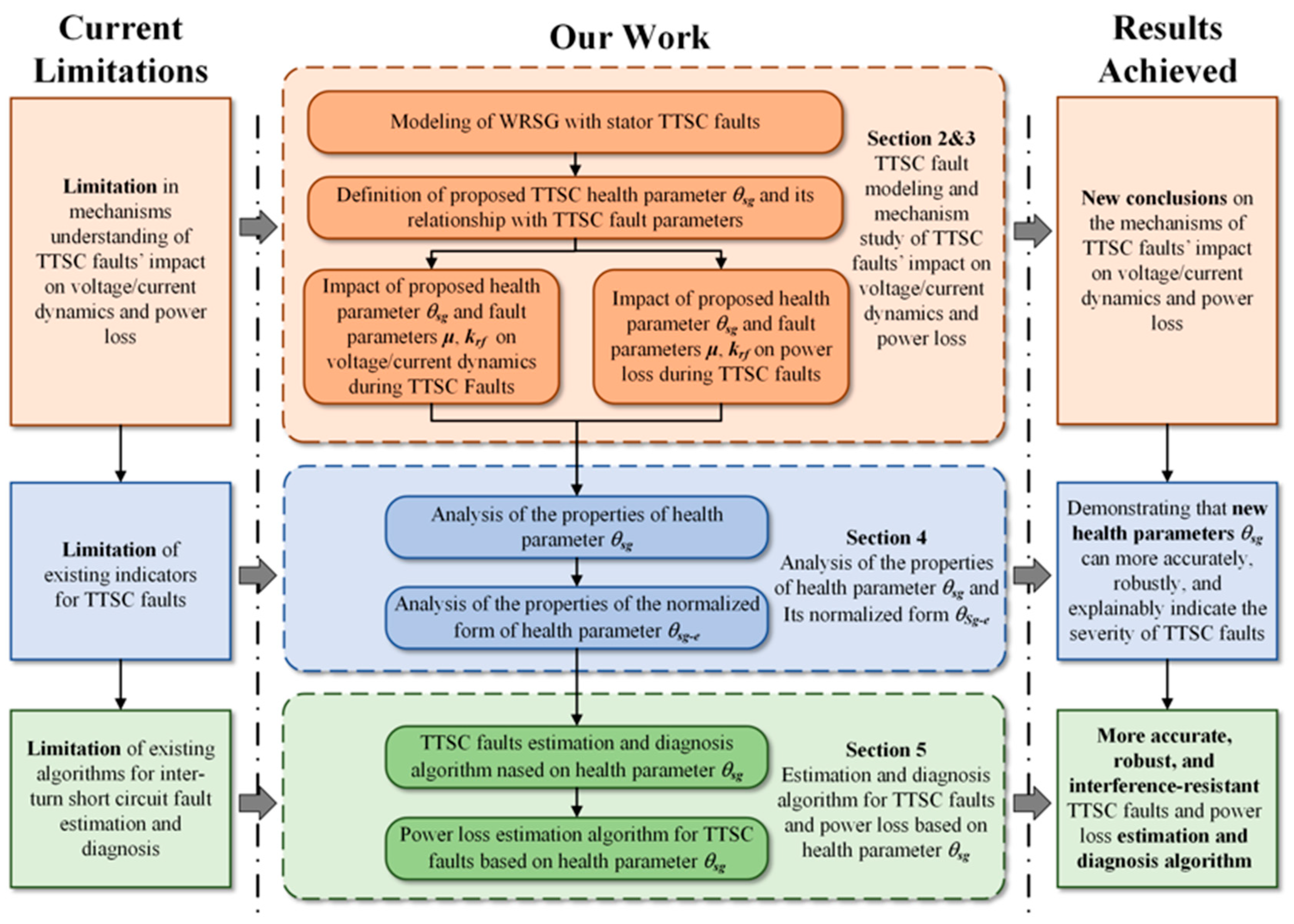
The research framework of this paper is shown in Figure 1, which introduces the main research problems addressed, the work conducted, the innovations implemented, and the achievements obtained in this study. Currently, research on the analysis, estimation, and diagnosis of generator stator TTSC faults has three major limitations. (1) A limited understanding of the TTSC fault mechanisms, manifested as an insufficient comprehension of how fault parameters affect the voltage, current, and the mechanisms of power loss caused by faults. (2) The limitations of existing TTSC fault indicators. Due to the aforementioned insufficient understanding, fault indicator parameters developed based on this cognition (such as zero-sequence voltage, negative-sequence voltage, and second harmonics) are susceptible to external interference and cannot accurately assess the severity of faults. (3) Limitations of the existing TTSC fault estimation and diagnostic algorithms. Since these algorithms are built upon the above-mentioned easily-interfered indicators, they generally suffer from poor accuracy, low stability, and weak anti-interference capabilities.
To address these three limitations, this paper systematically conducted the following three targeted research efforts in sequence, yielding three innovative achievements. First, to resolve the insufficient understanding of fault influence mechanisms, Section 2 and Section 3 deeply analyze the relationship between the fault parameters and fault voltage/current dynamics as well as the relationship between the fault parameters and power loss. We propose a new TTSC fault health parameter and thoroughly explore the correlation between the health parameter and voltage/current dynamics and power loss, thereby gaining new insights into how TTSC faults affect the voltage and current characteristics. Second, regarding the limitations of the existing fault indicators, Section 4 presents an in-depth theoretical analysis of the properties of the proposed health parameter and its normalized forms, demonstrating that the parameters offer greater accuracy, robustness, and interpretability compared with traditional fault indicators. (3) Based on the above research findings, Section 5 focuses on addressing the limitations of the existing fault estimation and diagnostic algorithms. Building upon the proposed health parameters, we designed TTSC fault and power loss estimation and diagnostic algorithms with higher accuracy, stronger robustness, and superior anti-interference capabilities.
These systematic research efforts, along with the resulting new understanding of fault mechanisms, new health parameter, fault evaluation systems, and new fault and power loss estimation and diagnostic algorithms, effectively address the deficiencies and limitations in the current research. Finally, in Section 6, we validate the above conclusions and achievements through extensive Monte Carlo simulations.

2. Model of WRSG with Stator TTSC Faults

In this section, we present a generic model of the WRSG capable of representing stator winding TTSC faults. The structure of the WRSG is shown in Figure 2, consisting of a main generator, load, exciter, and an automatic voltage regulator (AVR). The main generator is responsible for supplying three-phase AC power to the load. The exciter provides excitation voltage to the field winding of the main generator rotor, thereby generating the magnetic field. The AVR acts as a controller to ensure that the output voltage remains within a specified range by controlling the excitation voltage of the exciter. Given that this study focused on stator TTSC faults in the main generator, we did not explicitly specify the structure and type of the AVR and exciter. Instead, the AVR and exciter were considered equivalent to an AC5A excitation voltage controller [4,47,48], and it was assumed that the output excitation voltage could be measured or estimated. We further assumed that the faults were incipient and that the generator possessed a degree of redundancy; consequently, the effects of the magnetic saturation were not taken into consideration [25]. These assumptions simplify the modeling complexity and enhance its generalizability. It is worth noting that due to these assumptions, our approach is primarily applicable for early-stage TTSC detection in generators operating within linear regimes, where nonlinear behaviors remain minimal.
We assumed that the main generator stator had three phases, namely s a , s b , and s c , which were used to output the three-phase alternating voltage/current, as depicted in Figure 2. The TTSC faults were assumed to occur in phase s a of the main generator, where the short-circuit branch had a resistance of R f and a current of I f . The ratio of the number of turns in the short-circuited section to the total number of turns N is denoted by μ . The short-circuited section in phase s a is referred to as s a f , while the healthy section is referred to as s a h . The directions of the respective currents are illustrated in Figure 3. We introduced the parameter k r f , which signifies the ratio of the resistance of the short-circuit branch to that of the short-circuit part of the coil, to compute R f , where R f = k r f μ r s . Consequently, the fault in the TTSC can be characterized by the fault parameters μ and k r f .
The main generator was modeled by using a widely adopted and validated multi-loop theory [25,49,50]. This approach assumes that the TTSC fault results in the formation of a new current path, as depicted in Figure 3, causing a diversion of current, and thus reducing the current flowing through the original turns. During this process, the number of turns in the faulty phase does not decrease. Based on this assumption, the multi-loop theory treats the short-circuit branch formed during a TTSC fault as a fault loop. Subsequently, by computing the coupling effects of the fault current in this loop with other parts of the generator, the operational state of the generator under this fault condition can be deduced. This methodology enables the representation of both normal scenarios (where the short-circuit branch resistance is near-infinite) and faulty scenarios (where the short-circuit branch resistance is relatively low).
Furthermore, the dq0 rotor reference frame was employed to reduce the complexity of the inductance matrix involved in the conversion of flux linkage and current, thus minimizing the utilization of computational resources. Furthermore, the orientation of coordinate axes and the directionality of various quantities are available in the reference to the IEEE standards [51]. In the following, we present the key governing expressions to characterize the dynamics of the generator.
The relationship between the voltage, current, and flux linkage of the armature winding of the main generator can be described by
V s q d 0 = W r λ s q d 0 + d λ s q d 0 d t T R s   T 1 i s q d 0 + T μ r s i f a b c + w 1
where
V s q d 0 = [ V s q , V s d , V s 0 ] T ,   λ s q d 0 = [ λ s q , λ s d , λ s 0 ] T ,   i s q d 0 = [ i s q , i s d , i s 0 ] T ,   i f a b c = [ i f , 0 , 0 ] T
R s = d i a g [ r s , r s , r s ] T ,   W r = 0 w r 0 w r 0 0 0 0 0
V s q , V s d , V s 0 denote the voltage of the stator winding in the dq0 rotating reference frame;
λ s q , λ s d , λ s 0 denote the flux linkage of the stator winding in the dq0 rotating reference frame;
i s q , i s d , i s 0 denote the current of the stator winding in the dq0 rotating reference frame;
T denotes the transformation matrix from the abc frame to the dq0 frame;
r s denotes the stator phase winding resistance;
w r denotes the generator speed;
w 1 denotes the noise indicating uncertainty.
The rotor of the main generator can be classified into two types, namely salient and round. Our research focused on the salient-pole rotor for subsequent investigation. It should be noted that the subsequent theoretical analysis and conclusions also held for the round structure. However, due to space limitations, we do not provide a separate demonstration for the round structure.
The relationship between the voltage, current, and flux linkage of the rotor winding in the generator is described by
V r q d 0 = d λ r q d 0 d t + R r i r q d 0 + w 2
where
λ r q d 0 = [ λ f d , λ k d , λ k q ] T ,   V r q d 0 = [ V f d , V k d , V k q ] T ,   i r q d 0 = [ i f d , i k d , i k q ] T , R r = d i a g [ r f d , r k d , r k q ] T
V f d , V k d , V k q denote the voltage of the rotor field winding, damper bars on the d-axis and q-axis;
λ f d , λ k d , λ k q denote the flux linkage of rotor field winding, damper bars on the d-axis and q-axis;
i f d , i k d , i k q denote the current of rotor field winding, damper bars on the d-axis and q-axis;
r f d , r k d , r k q denote the resistance of rotor field winding, damper bars on the d-axis and q-axis;
w 2 denotes the noise indicating uncertainty.
The relationship between the flux linkage and current in the generator can be expressed by
λ s , r q d 0 = L ( i s , r q d 0 K 1 T ( : , 1 ) μ i f )
where
i s , r q d 0 = [ i s q , i s d , i s 0 , i f d , i k d , i k q ] T
λ s , r q d 0 = [ λ s q , λ s d , λ s 0 , λ f d , λ k d , λ k q ] T
K 1 = 1 0 0 0 0 0 0 1 0 0 0 0 0 0 1 0 0 0 T
T ( : , 1 ) is the first column of the matrix T, and
L = ( L m q + L l s ) 0 0 0 0 L m q 0 ( L m d + L l s ) 0 L m d L m d 0 0 0 L s 0 0 0 0 L m d 0 ( L m d + L l f d ) L m d 0 0 L m d 0 L m d ( L m d + L l k d ) 0 L m q 0 0 0 0 ( L m d + L l k q )
Equations (1)–(3) determine the voltage–current relationship of the generator. It should be noted that as this study focused on the initial stages of the TTSC malfunction, the inductance matrix did not take into account the effects of distortion in the space harmonics and air-gap flux density disturbance, among others that are caused by the TTSC [14,25,52]. However, our theory is applicable to any form of inductance matrix, and hence is capable of being extended. This suggests that, if necessary, more accurate results that consider the effects of distortion and air-gap flux density disturbances can be obtained by integrating other analytical methods, such as the winding function approach (WFA), to refine the inductance matrix [4]. However, while our method has extension potential, this paper specifically focused on the current assumptions, namely ignoring the aforementioned effects and concentrating on early-stage TTSC faults.
Due to presence of stator TTSC faults, the above equations contain parameters that are related to the fault. To investigate the above equation, it is necessary to introduce the following equations to describe the fault circuit, namely
d λ s a f d t μ r s ( i a i f ) = R f i f
where λ s a f denotes the flux linkage of the faulty winding a s f in phase s a .
Equations (1)–(4) determine the current–voltage dynamics of the main generator. Subsequently, to model the voltage–current characteristics of general electrical loads, rather than focusing on specific load structures, a state-space approach was employed here to represent various types of electrical loads and their voltage–current characteristics, as shown in Equation (5) [53,54], where x l o a d represents the load state variables, which may include voltage, current, and other load-specific states depending on the particular load characteristics. The corresponding generator terminal measurements of voltage and current can be expressed by using Equation (6). By simultaneously solving Equations (1)–(6), the voltage–current dynamics and measurements of the entire system can be obtained.
d x l o a d d t i s a b c = f l o a d x l o a d , V s a b c g l o a d ( x l o a d , V s a b c )
i ˜ s a b c V ˜ s a b c , f d = i s a b c V s a b c , f d + v i v v
where
V s a b c , f d = [ V s a , V s b , V s c , V f d ] T , i s a b c = [ i s a , i s b , i s c ] T .
f l o a d , g l o a d , x l o a d is the characteristic equation of the electrical load and its state variables;
V s a , V s b , V s c denote the terminal voltage of the three-phase;
i s a , i s b , i s c denote the terminal current of the three-phase;
v i , v v denote the uncertainty associated with current and voltage measurements, respectively;
~ is the superscript of the measured values.
Equations (1)–(5) provide and define the system, where the solutions to these equations represent the dynamic voltage and current of the system. Equation (6), on the other hand, provides the relationship between the measured values and the true values of the voltage and current. Based on these equations, we constructed a WRSG model in MATLAB/Simulink to solve these equations and simulate the TTSC faults.

3. Impact of the Health Parameter θsg and Fault Parameters μ and krf on the Voltage, Current, and Power Loss During TTSC Faults

The health parameter proposed for WRSG TTSC faults is as follows:
θ s g = k r f + 1 μ
We now analyze how the proposed health parameter θ s g correlates with the dynamics of the current and voltage as well as the power loss during the stator TTSC faults, and also explore the interplay between these electrical characteristics and fault parameters μ and k r f . First, we will show that regardless of the power load type, whether linear or nonlinear, identical current and voltage dynamics can correspond to an infinite number of TTSC faults, each characterized by distinct fault parameters. This implies that the two fault parameters μ and k r f of the stator TTSC cannot be determined solely by measuring the terminal voltage and current. Second, we will show that by keeping all other factors unchanged, the dynamic behavior of the voltage and current during the stator TTSC faults can be determined by the proposed health parameter θ s g . Finally, we will show that the magnitude of the power loss in the stator TTSC is also determined by the proposed health parameter θ s g .

3.1. Impact of Health Parameter θsg and Fault Parameters μ and krf on the Voltage–Current Dynamics During TTSC Faults

In this subsection, we will, on the one hand, show that the value of the proposed health parameter determines the impact of the TTSC faults on the dynamics of the voltage and current within the system. On the other hand, we will present evidence to demonstrate that the two parameters of the TTSC faults μ , k r f cannot be exclusively determined based on the generator’s measured current and voltage. We now state our first main result.
Theorem 1.
For the WRSG system, as defined by Equations (1)–(6), under the assumption that noise is not considered (i.e., w 1 , w 2 , v i , and v v are set to zero), and the health parameter θ s g , the electrical load and other system parameters are the same, with the exception of the fault parameters μ and k r f , then it follows that the solutions for the system voltage and current dynamics V s , r q d 0 , i s , r q d 0 , and the flux linkage λ s , r q d 0 are the same, regardless of the values of fault parameters μ and k r f .
Proof. 
Equations (1) and (2) can be incorporated to obtain
V s , r q d 0 = R i s , r q d 0 + W r λ s , r q d 0 + d λ s , r q d 0 d t + K 1 T ( : , 1 ) μ r s i f + w s , r
where
V s , r q d 0 = [ V s q , V s d , V s 0 , V f d , V k d , V k q ] T ,   i s , r q d 0 = [ i s q , i s d , i s 0 , i f d , i k d , i k q ] T
R = d i a g [ r s , r s , r s , r f d , r k d , r k q ] T ,   W r = K 1 T W r ,   and   w s , r = [ w 1 , w 2 ] T .
Clearly, Equation (7) is equivalent to Equations (1) and (2). This implies that the generator system, constituted by Equations (1)–(6), is equivalent to the system formed by Equations (3)–(7), having the same solutions for V s , r q d 0 , i s , r q d 0 , and λ s , r q d 0 .
By multiplying both sides of Equation (7) by T ( 1 , : ) 1 and combining it with Equation (4), we can derive the following:
T ( 1 , : ) 1 V s q d 0 = T ( 1 , : ) 1 W r λ s q d 0 + T ( 1 , : ) 1 d λ s q d 0 d t T ( 1 , : ) 1 T R s   T 1 i s q d 0 + T ( 1 , : ) 1 T μ r s i f a b c + T ( 1 , : ) 1 w 1 V s a = T ( 1 , : ) 1 W r λ s q d 0 + T ( 1 , : ) 1 ( d T d t λ s , r a b c + T d λ s , r a b c d t ) r s i s a + μ r s i f + T ( 1 , : ) 1 w 1 V s a = T ( 1 , : ) 1 W r λ s q d 0 + T ( 1 , : ) 1 d T d t λ s , r a b c + 1 μ [ R f i f + μ r s ( i a i f ) ] r s i s a + μ r s i f + T ( 1 , : ) 1 w 1
where λ s a represents the flux linkage of the a-phase winding.
After some algebraic manipulations, the following equation can be derived:
μ i f = V s a T ( 1 , : ) 1 W r λ s q d 0 T ( 1 , : ) 1 d T d t λ s , r a b c T ( 1 , : ) 1 w 1 r s ( 1 ( k r f + 1 μ ) )
Given the following equation,
T ( 1 , : ) 1 W r λ s q d 0 T ( 1 , : ) 1 d T d t λ s , r a b c = ( T ( 1 , : ) 1 W r + T ( 1 , : ) 1 d T d t T 1 ) λ s , r q d 0 = 0
Equation (9) can be simplified into the following:
μ i f = V s a T ( 1 , : ) 1 w 1 r s ( 1 θ s g )
Clearly, the solutions for the system of Equations (3)–(7), which represent the system dynamics V s , r q d 0 , i s , r q d 0 , and λ s , r q d 0 , also satisfy the system of Equations (3), (5)–(7), and (11). It can be inferred from Equations (8) to (11) that the converse is also true. Thus, the two systems are equivalent and possess the same solutions.
Observing the system of equations that is composed of Equations (3), (5)–(7), and (11), it follows that when w 1 , w 2 , v i , and v v are set to zero, and given that the health parameter θ s g , electrical load, and other system parameters are the same, with the exception of μ and k r f , the system solutions remain the same. This suggests that under these conditions, the system voltage, current, and flux linkage dynamics remain unchanged. Due to the above equivalence that has been demonstrated, this completes the proof of the theorem. □
Consequently, we have demonstrated that the proposed health parameter θ s g determines the impact of the TTSC faults on the system terminal voltage and current. With the electrical load and other parameters held constant, θ s g dictates the voltage and current dynamics of the system during the stator TTSC faults.
Theorem 2.
For the WRSG system, as defined by Equations (1)–(6), under the assumption that noise is not considered (i.e., w 1 , w 2 , v i , and v v are set to zero), and the health parameter θ s g , the electrical load and other system parameters are the same, with the exception of fault parameters μ and k r f , then it follows that if the system voltage dynamics V s , r q d 0 , the current dynamics i s , r q d 0 are the same, then the fault parameters μ and k r f have infinite sets of solutions.
Proof. 
From Equations (3) to (7) and (11), it follows that for any voltage and current values V s , r q d 0 and i s , r q d 0 , there always exists a θ s g that corresponds to these values. According to the definition, this θ s g corresponds to an infinite number of solutions for μ and k r f . Therefore, the same V s , r q d 0 and i s , r q d 0 correspond to an infinite number of solutions for μ and k r f . This completes the proof of the theorem. □
Consequently, we have demonstrated that the two parameters μ and k r f of the TTSC faults cannot be determined solely based on the current and voltage measurements of the generator. Thus far, we demonstrated that the value of the health parameter θ s g determines the impact of the TTSC faults on the terminal voltage and current of the generator. We have also shown that it is impossible to determine the two fault parameters μ and k r f of the stator TTSC solely based on the voltage and current measurements. This is the case even with different TTSC faults (i.e., different μ and k r f ), where as long as their corresponding health parameter θ s g is the same, the system voltage and current dynamics remain identical.

3.2. Impact of Health Parameter θsg and Fault Parameters μ and krf on Power Loss During TTSC Faults

Our goal was to demonstrate that although one cannot accurately estimate the two fault parameters μ and k r f of the TTSC faults based solely on the measured current and voltage of the generator, one can still estimate the power loss caused by the stator TTSC faults by using the proposed health parameter θ s g and the measured voltage and current signals.
First, we define the power loss caused by the TTSC faults as the sum of the energy loss caused by the short-circuited portion of the circuit and the additional power loss due to the presence of the short-circuit current in the stator winding [30]. The governing expression is as follows:
P l o s s = i f 2 r f + ( i a i f ) 2 r s a f i a 2 r s a f
where r s a f = μ r s represents the resistance value of the faulty portion of the stator winding in the phase s a .
Theorem 3.
For the WRSG system, as defined by Equations (1)–(6), under the assumption that noise is not considered (i.e., w 1 , w 2 , v i , and v v are set to zero), and the health parameter θ s g , the electrical load and other system parameters are the same, with the exception of fault parameters μ and k r f , then it follows that the power loss of the generator caused by the TTSC faults P l o s s remains the same, regardless of the value of fault parameters μ and k r f .
Proof. 
Equation (12) can be rearranged as follows:
P l o s s = i f 2 r f + ( i a i f ) 2 r s a f i a 2 r s a f = i f 2 r f + i f 2 μ r s + i a 2 μ r s 2 i a i f μ r s i a 2 μ r s = r s ( μ i f ) 2 θ s g 2 i a r s μ i f
Therefore, based on Theorem 1, it can be inferred that both i a and μ i f yield identical solutions under the above conditions. Therefore, under these circumstances, the value of P l o s s remains the same. This completes the proof of the theorem. □
By leveraging Theorem 3 and incorporating Equations (5) and (11), one can readily derive the following corollary.
Corollary 1.
For the WRSG system, as defined by Equations (1)–(6), under the assumption that noise is not considered (i.e., w 1 , w 2 , v i , and v v are set to zero), and the value of the healthy parameter θ s g , along with the measured voltage and current V ˜ s a b c , f d , i ˜ s a b c of the generator is known, then it follows that the power loss caused by the stator TTSC faults in the generator can be estimated, even without knowing the exact values of μ and k r f .
Consequently, we have demonstrated that the healthy parameter θ s g determines the power loss in the generator caused by TTSC faults. Even though one cannot accurately determine the parameters μ and k r f , it is still possible to accurately estimate the power loss that is caused by the TTSC faults by using the healthy parameter θ s g .

4. Characteristics and Normalized Form of the Health Parameter θsg

In this section, we describe and present the three beneficial characteristics of the proposed health parameter θ s g . Subsequently, we introduce the normalized form of this parameter and discuss its functionality.

4.1. Characteristics of the Health Parameter θsg

Specificity and Robustness: Under the condition that all other factors remain unchanged, the health parameter value is specific, with each health parameter value corresponding to a determined terminal voltage/current response. There is no identical health parameter that corresponds to different terminal voltage/current dynamics and impacts. Furthermore, the proposed health parameter exhibits robustness and a high degree of resistance to extraneous factors. Furthermore, it reliably indicates the degree of stator TTSC faults across a variety of conditions.
Quantifiability and Monotonicity: The health parameter is quantifiable and monotonic in nature to allow for an objective and quantitative assessment of the system health and performance. This quantification and monotonicity enable an effective comparison between different levels of the fault severity. For instance, as the severity of the fault increases (or decreases), the corresponding value of the health parameter also increases (or decreases).
Universality and Interpretability: The health parameter is universalizable, implying that it can be applied to the WRSG of different sizes or configurations. The health parameter is also easily interpretable, providing information with clear physical significance regarding the condition of the generator, thereby facilitating relevant decision-making processes for health monitoring and diagnosis.
Next, we demonstrate that the proposed health parameter possesses the above characteristics. Based on Theorem 1, one can substantiate that the proposed health parameter θ s g is capable of uniquely determining the terminal current and voltage dynamic responses. Therefore, our health parameter exhibits specificity. Given that the proposed health parameter is derived solely from the fault parameters, its values are not influenced by external factors. Consequently, these parameters provide a consistent and stable indication of the severity of the TTSC fault under various operational conditions, exhibiting exceptional robustness.
In order to substantiate that our health parameter exhibited quantifiability and monotonicity, it was necessary to define the criteria to evaluate the severity of two TTSC faults. We assumed that for two TTSC faults, T f a u l t 1 and T f a u l t 2 , their severity levels were I T f a u l t 1 and I T f a u l t 2 , respectively, and the associated fault parameters were μ 1 , k r f 1 and μ 2 , k r f 2 , respectively. The power losses P l o s s T f a u l t 1 and P l o s s T f a u l t 2 occurred under the same fault output voltage V s a and current i a . Subsequently, we conducted comparisons under four different scenarios.
Scenarios 1: If μ 1 = μ 2 , k r f 1 = k r f 2 , it was assumed that I T f a u l t 1 = I T f a u l t 2 .
Scenarios 2: If μ 1 = μ 2 , k r f 1 k r f 2 , it was assumed that I T f a u l t 1 < I T f a u l t 2 when k r f 1 > k r f 2 . Conversely, when k r f 1 < k r f 2 , then I T f a u l t 1 > I T f a u l t 2 .
Scenarios 3: If μ 1 μ 2 , k r f 1 = k r f 2 , it was assumed that I T f a u l t 1 > I T f a u l t 2 when μ 1 > μ 2 . Conversely, when μ 1 < μ 2 , then I T f a u l t 1 < I T f a u l t 2 .
Scenarios 4: If μ 1 μ 2 , k r f 1 k r f 2 , it was assumed that when P l o s s T f a u l t 1 > P l o s s T f a u l t 2 , then I T f a u l t 1 > I T f a u l t 2 and when P l o s s T f a u l t 1 < P l o s s T f a u l t 2 , then I T f a u l t 1 < I T f a u l t 2 and when P l o s s T f a u l t 1 = P l o s s T f a u l t 2 , then I T f a u l t 1 = I T f a u l t 2 .
The reasons for choosing the above comparison criteria were as follows. In the first three scenarios, we could directly compare them based on our intuitive understanding of the TTSC faults. When the ratio of the short-circuit turns and ratio of the short-circuit branch resistance was the same, the fault parameters were completely identical, resulting in the same severity of the fault. When the ratio of the short-circuit turns was fixed, the fault with a lower ratio of the short-circuit branch resistance was more severe. When the ratio of the short-circuit branch resistance was the same, the fault with a higher ratio of short-circuit turns was more severe. However, in the fourth scenario, where both the short-circuit turns and short-circuit branch resistance were different, a direct comparison was not possible. Therefore, one needs to choose a metric to evaluate, and in this scenario, we chose the power loss caused by the TTSC.
The above reasoning was based on the fact that power loss directly affects the efficiency of the generator, which in turn affects the operation of the system. Additionally, the power loss also leads to extra heat generated by the fault. The significant increase in this heat poses a severe challenge to the safe operation of the generator. Therefore, power loss is an excellent reference value for measuring the impact and severity of the fault [30,55]. It follows that under the same fault voltage and current conditions, a fault with a higher power loss is more severe, while faults with the same power loss have the same severity.
Subsequently, we will demonstrate that the proposed health parameter θ s g satisfied the requirements of quantifiability and monotonicity under the above comparison rules. Upon examining the definition of θ s g , it was evident that the first three scenarios all met the criteria of quantifiability and monotonicity. Therefore, we will now proceed to show that the quantifiability and monotonicity still held for scenario 4.
Upon analysis of the health parameter θ s g , it was observed that it decreased with the increase in the short-circuit range μ , and with the decrease in the short-circuit resistance k r f . This suggests that as the severity of TTSC faults increases, the value of the health parameter consistently declines. The maximum value of the health parameter is achieved when the short-circuit range μ approaches zero and the short-circuit resistance k r f approaches infinity, representing an ideal state of health with a maximum value of + . Conversely, the minimum value of the health parameter occurs when the short-circuit range μ = 1 , indicating a full-phase short circuit, and when the k r f resistance is 0, this represents an ideal state of the maximum fault with a minimum value of 1. Therefore, the health parameter ranges within the interval [ 1 , + ) , where 1 designates an ideal state of a complete short circuit, and + represents an ideal state of the complete health.
Upon substituting Equation (11) into Equation (13), one is able to derive the following expression:
P l o s s = V s a T ( 1 , : ) 1 w 1 ( θ s g 1 ) ( V s a T ( 1 , : ) 1 w 1 r s ( 1 1 θ s g ) 2 i a )
From Equation (14), it follows that under the same voltage V s a and current i a , the power P l o s s progressively increases as the health parameter θ s g decreases from + to 1 . Thus, in conjunction with the above analysis and evaluation criteria, one can conclude that the severity of a fault escalates with the decrease in the health parameter θ s g . As the fault phase progresses from a healthy state to a complete short circuit, indicating an escalating severity, the health parameter θ s g correspondingly decreases from + to 1 . Consequently, we were able to validate that our proposed health parameter θ s g adheres to quantifiability and monotonicity.
Based on the observations and conclusions above, an additional benefit of using the power loss as an assessment metric became evident, namely it aligned with the criteria corresponding to the other three scenarios. Specifically, for higher severe faults occurring within these scenarios, there was a corresponding increase in the power loss.
As demonstrated in Section 2 and Section 3, our proposed health parameter can be applied to various types of loads, exciters, and AVR, thereby exhibiting strong universality. Moreover, an observation of θ s g revealed that this health parameter is independent of any other generator parameter and relies solely on the fault branch resistance ratio k r f and the short-circuit turns ratio μ . These parameters are universal for TTSC faults, hence, θ s g displays a high degree of universality, can be applied in generators with different parameters, and exhibits broad representativeness. An identical health parameter θ s g value corresponds to a similar degree of TTSC faults, which demonstrates its universality. As previously illustrated, θ s g is a value that gradually changes from + to 1 as the fault severity increases, thereby making θ s g have direct physical meanings that are clear and interpretable. Consequently, we validated that θ s g possesses both universality and interpretability.
The above properties endowed our proposed health parameter with superior capabilities for assessing stator TTSC faults in the WRSG compared with traditional fault indication signals such as the zero-sequence voltage [14,39]. These assertions will also be validated in Section 6.

4.2. Normalized Form of the Health Parameter θsg

In the realm of fault diagnosis technology, the aim is to make health parameters more intuitive. Consequently, we proposed a normalized form, denoted by θ s g e , of the health parameter θ s g . Unlike θ s g , θ s g e is a parameter ranging from 0 to 1. The corresponding normalized form for the proposed health parameter is now given as follows:
θ s g e = 1 e ( 1 θ s g ) / k e
where k e denotes a scaling coefficient.
Given that the health parameter θ s g and its normalized counterpart θ g s e have a monotonic and bijective mapping, it can be inferred that the normalized form of the health parameter θ s g e also adheres to all previously identified characteristics pertaining to θ s g .
When θ s g e equals 1, it signifies an healthy state, with no short-circuit occurrence. As θ s g e decreases, the magnitude of the TTSC fault progressively increases. When θ s g e diminishes to 0, it indicates a complete short-circuit fault in the phase (i.e., the short-circuit turns ratio is 1, and the short-circuit branch resistance ratio is 0). Consequently, compared with θ s g , its normalized form θ s g e is more intuitive.
The scaling factor k e in θ s g e is utilized to adjust the sensitivity of θ s g e to incipient faults. A larger k e increases the sensitivity of θ s g e to incipient faults, resulting in a faster decay during early faults. Conversely, a smaller k e reduces the sensitivity of θ s g e to incipient faults, requiring a more significant fault to cause a noticeable decrease in θ s g e . In this study, k e was 10 4 .
In summary, when we aim to express the fault degree more intuitively, θ s g e can replace θ s g . This normalized health parameter can be used to describe TTSC faults in WRSG, offering superior interpretability and intuitiveness.
Here, we would like to provide a more intuitive explanation of the physical meaning behind our health parameters θ s g and θ s g e . θ s g can be understood as an abstract-level short-circuit resistance obtained by weighting the short-circuit branch resistance k r f with the shorted turn ratio μ . The larger this abstract-level short-circuit resistance, the smaller the short-circuit magnitude. When this short-circuit resistance approaches infinity, there is naturally no short circuit; when it equals zero, it indicates a complete short circuit. Meanwhile, θ s g e can be viewed as a normalized form of θ s g , designed for easier practical use. A value of 1 represents complete health, while a value of 0 represents a complete short circuit—the worst health condition. This approach is similar to various health parameters used in the industry, making it more intuitive to understand and implement.

5. Estimation Algorithm for the Health Parameter θsg and Power Loss Ploss

In this section, we present the proposed estimation method based on the Kalman filter (KF) for estimating the proposed health parameter and power loss, followed by an analysis of their associated errors.
Let us express the current–voltage characteristic Equations (1)–(3) of the generator as follows:
d λ s , r q d 0 d t = V s , r q d 0 + R i s , r q d 0 W r λ s , r q d 0 K 1 T ( : , 1 ) μ r s i f w s , r
i s , r q d 0 = L 1 ( λ s , r q d 0 + L K 1 T ( : , 1 ) μ i f )
By treating the measured voltage in Equation (6) as the input and the measured current as the output and substituting them into Equations (15) and (16), with the flux linkage considered as the state variable, the current–voltage characteristic equation of the generator can be expressed in the state-space representation given by Equations (17) and (18) after some algebraic manipulation, as follows:
d λ s , r q d 0 d t = K 2 T 2 V ˜ s a b c , f d + ( R L 1 W r ) λ s , r q d 0 w s , r + K 2 T 2 v v
i ˜ s a b c = T 1 K 1 T L 1 ( λ s , r q d 0 + L K 1 T ( : , 1 ) μ i f ) v i
where K 2 = d i a g ( 1 , 1 , 1 , 1 )         0 4 × 7 T and T 2 = T 0 0 1 .
Upon substituting μ i f in Equation (18) with Equation (11), one can derive the following:
i ˜ s a b c = T 1 K 1 T L 1 λ s , r q d 0 + K 3 V s a T ( 1 , : ) 1 w 1 1 θ s g v i
By considering 1 1 θ s g as an augmented state variable x f , the state-space Equations (17) and (18) can be further expressed in the following form:
d x a u g d t = A x a u g + B V ˜ s a b c , f d + w n
i ˜ s a b c = C x a u g K 3 T ( 1 , : ) 1 x f w 1 v i
where
x a u g = [ λ s , r q d 0 T , x f ] T ,   A = R L 1 W r 0 0 0 ,   B = K 2 T 2 ,   C = T 1 K 1 T L 1 K 3 V s a
w n = [ ( w s , r + K 2 T 2 v v ) T , 0 ] T ,   and   K 3 = [ 1 r s , 0 , 0 ] T .
In the above system, the only nonlinear component is denoted by K 3 T ( 1 , : ) 1 x f w 1 . Given the assumption that the fault was not excessively severe and that the magnetic saturation effects were absent, it was evident that x f << 1. The term w 1 represents noise, which is also a relatively low magnitude quantity. Consequently, the impact of this nonlinear component on the system was considered negligible. For the sake of reducing the computational cost and complexity of proposed algorithms, we opted to disregard this nonlinearity. Hence, the system can be represented in the following linearized form in Equations (22) and (23):
d x a u g d t = A x a u g + B V ˜ s a b c , f d + w n
i ˜ s a b c = C x a u g v i
Subsequently, for a continuous generator system, one can employ a KF to estimate the augmented state, x a u g , of the system. The KF algorithm utilized for estimating x a u g involves the following update Equations (24)–(26) for the covariance matrix, the KF gain, and the state estimate x ^ a u g [56], namely
P ˙ = F P + P F T + Q ( P C T ) R 1 ( P C T ) T
K = ( P C T ) R 1
x ^ ˙ a u g = A x ^ a u g + B V ˜ s a b c , f d + K ( i ˜ s a b c C x ^ a u g )
where Q and R are matrices representing the intensity of noise for w n and v i , respectively, where the superscript ^ denotes the estimated value.
Upon obtaining the estimate of x a u g through the application of the KF, we are then able to derive the estimate of x f . Subsequently, an estimate of the parameter θ s g and the power loss P l o s s can be ascertained by using the following equations.
θ ^ s g = 1 1 x ^ f
P ^ l o s s = V ˜ s a 2 r s ( 1 θ ^ s g ) 2 θ ^ s g ( t ) 2 i ˜ a V ˜ s a ( 1 θ ^ s g )
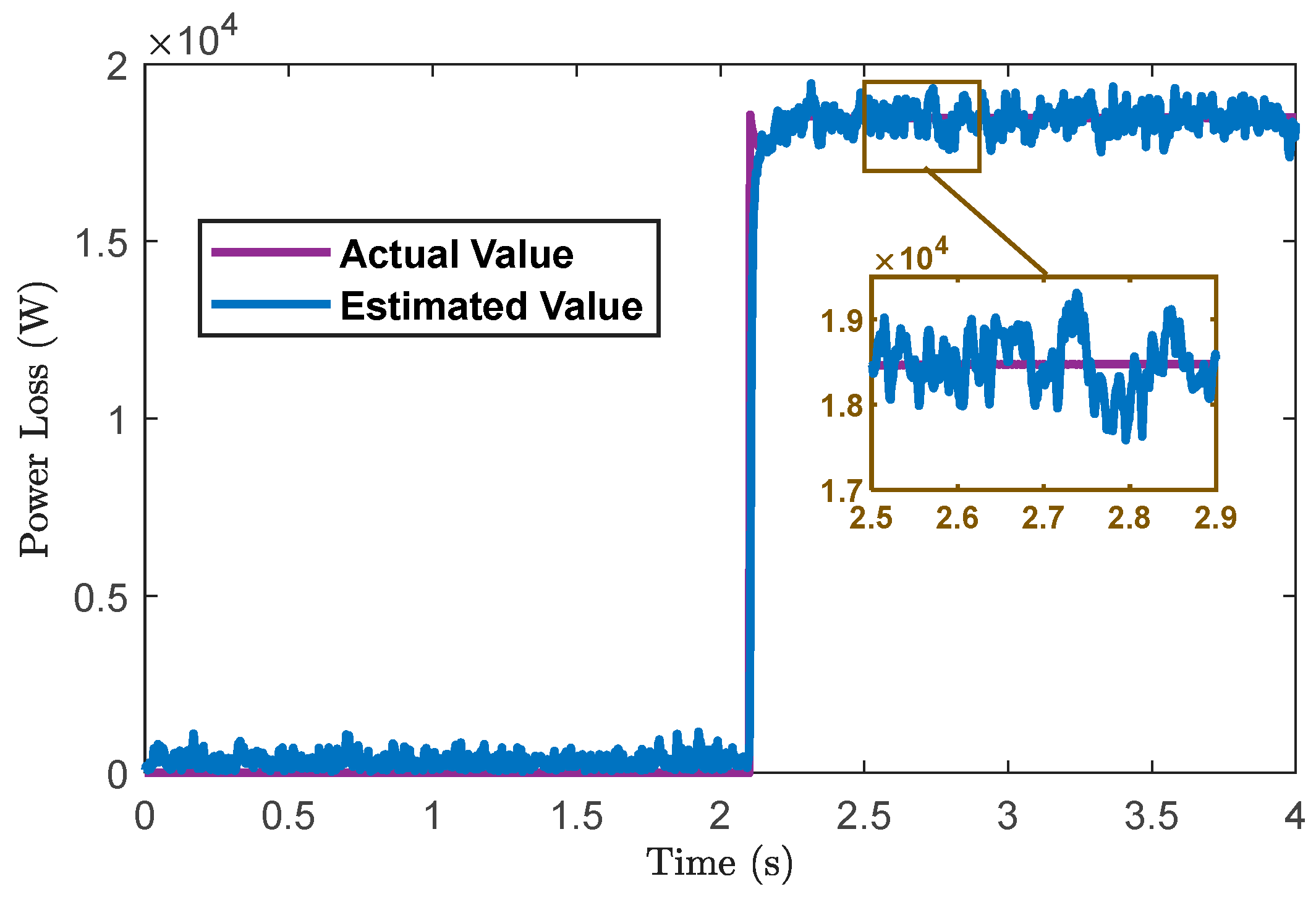
The complete estimation algorithm is outlined in Algorithm, as shown in Figure 4. It must be noted that due to the characteristics of probability distributions, the estimates of θ s g and P l o s s derived from x f using Equations (26) and (27) are not unbiased and are subject to error. However, the simplicity and computational efficiency of the above method for estimating θ s g and the power loss P l o s s from x f make it a viable option, particularly when the estimation error of x f remains small. Consequently, this method was retained for subsequent use in this study. For more precise estimates and to understand the distribution of these estimates, Monte Carlo sampling techniques can be employed to derive more reliable estimates of θ s g and the power loss from x f [57].
It is important to further note that, as mentioned in Section 2, the excellent properties of our proposed health parameters and the algorithm developed for estimating TTSC fault severity and power loss are based on the assumption that the TTSC fault is in its early, low-magnitude stage, and that the generator possesses a degree of redundancy. Consequently, the effects of magnetic saturation were not taken into consideration [25], and we also ignored the space harmonics and air-gap flux density disturbance, among other factors caused by the TTSC [14,25,52]. Therefore, if the TTSC fault becomes more severe, this method cannot be directly applied and would require further research and adjustments.

6. Simulation Results

In this section, we employed MATLAB/Simulink simulations to comprehensively validate our methodology through three detailed case studies and two Monte Carlo simulation evaluations. First, the structure and parameters of our detailed simulation model are presented, and then the case studies. Case Study 1 validated the effectiveness and characteristic properties of the proposed health parameter θsg introduced in previous sections, demonstrating its specificity in determining system dynamics under fault conditions. Case Study 2 evaluated the performance and accuracy of our estimation algorithm in quantifying both the health parameter θsg and power losses Ploss due to TTSC faults under various noise conditions. Case Study 3 further validated the robustness of our approach under dynamic loading/unloading conditions with different load types. Following these case studies, we conducted two Monte Carlo simulations to systematically compare our proposed FDI approach with traditional zero-sequence voltage methods, demonstrating the superior FDI capabilities of our method, particularly under unbalanced conditions and in the presence of disturbances. Specifically, Monte Carlo simulation 1 evaluated the performance under balanced linear load conditions, while Monte Carlo simulation 2 examined the robustness under imbalanced nonlinear loads. Through these extensive simulations, we were able to verify and validate the systematic theoretical framework proposed in this paper and its advantages over traditional approaches.

6.1. Verification and Validation of the Health Parameter θsg Characteristics and Estimation Algorithm

In this subsection, case study simulations were conducted to verify and validate the specificity of our proposed health parameter and the efficacy of our proposed estimation algorithm.
Drawing upon the established theoretical framework, we developed a model for the WRSG stator TTSC faults in the MATLAB/Simulink environment. This model comprises three main components, namely, the WRSG, the electrical load, and the fault estimator. The structure of this model is depicted in Figure 5. The WRSG component includes an excitation system based on the AC5A model, the input/output processing system, the electromagnetic and mechanical computing systems, and the Simscape electrical solver provided by Simulink. The parameters for the WRSG, derived from [52], are listed in Table 2. The electrical load was configured according to varying requirements, which will be detailed subsequently. The fault estimator, constructed by using Algorithm in Figure 4, was designed to estimate the proposed health parameter and the power loss due to TTSC faults.
Subsequently, we verified and validated the specificity of the proposed health parameter based on this model. Moreover, we assessed the accuracy of the newly introduced estimation algorithm that was used to estimate both the proposed health parameter and power loss.
Case Study 1: Initially, we set the noise level within the generator model to zero and connected the generator to a nonlinear, asymmetric, and unbalanced load, as depicted in Figure 6. This load comprises two parts: first, a balanced three-phase resistive load with a rating of 150 kW, operating at the generator’s nominal voltage and frequency, and second, a series connection of a diode and a resistive load, rated at 20 kW, also operating at the nominal voltage and frequency, connected across phases B and C.
Building on this setup, we conducted simulations for two distinct scenarios. In Scenario 1, the initial values of μ and the k r f were set to 0.1 and 5 × 10 6 , respectively. Subsequently, from 2 s to 2.1 s, k r f was rapidly decreased to 75 and maintained at this level until the end of the simulation time. In Scenario 2, the initial values of μ and k r f were set at 0.02 and 5 × 10 6 , respectively. Following this, starting from 2 s, k r f was rapidly decreased to 14 and then consistently maintained throughout the remainder of the simulation time. The changes in the fault parameters μ and k r f in the two scenarios are depicted in Figure 7.
Given that the initial values of k r f for both scenarios were set at 5 × 10⁻⁶—an extremely large number—the simulations initially represented the system’s healthy state prior to the occurrence of TTSC faults. From 2.1 s onward, the simulations reflected two distinct TTSC faults, each characterized by different fault parameters. However, due to our design, the health parameter θ s g for both faults remained identical.
Figure 8 and Figure 9 illustrate the dynamics of the system current, voltage, and power loss under Scenarios 1 and 2, respectively. The graphs revealed that following the fault occurrence, both the system voltage and current experienced a decline due to the fault but returned approximately to their nominal values under the control of the excitation controller. Throughout the simulations, the dynamics of the voltage and current as well as the power losses caused by the faults were nearly identical for both Scenarios 1 and 2.
The root mean square relative error (RMSRE) between the two scenarios is presented in Table 3, which was lower than the relative tolerance threshold of 0.1% established for the simulation solver. Therefore, we confirmed our proposed solution, where the health parameter θ s g is the key determinant of the fault impact and system dynamics. When other the conditions remained constant, consistent system dynamics were observed if the TTSC faults corresponded to an identical health parameter θ s g .
Case Study 2: In subsequent simulations, we varied both the noise associated with the flux linkage expression and the measurement noise of the generator from 0 to 5% of their maximum values under normal operating conditions. Next, we set all of the other parameters the same as in Scenario 1 in Case 1 and employed our proposed estimation algorithm to assess the health parameter θ s g of the generator, its normalized form θ s g e , and the power loss P l o s s attributed to the faults. Figure 10 and Figure 11 illustrate the estimation results, and Table 4 provides the precision of the proposed estimation algorithm. Given the previously stated consistency in system dynamics between Scenario 2 and Scenario 1, we will forego redundant simulations for Scenario 2.
As illustrated in Figure 10a, following the occurrence of the fault, our proposed estimation algorithm successfully estimated the system health parameter θ s g . Prior to the fault occurrence, due to a very high value of k r f , indicating the absence of an inter-turn short circuit fault, the fault current was minimal, resulting in a fault signature that was easily obscured by noise. Consequently, an accurate estimation of θ s g is challenging at this stage. The estimated value of θ s g at this point, which was about 8 × 10 4 , significantly deviated from the actual value of 10 7 , as seen in the figures. However, since the estimated θ s g remained at nearly 10 5 , relatively high, it did not impact our assessment adversely. Therefore, we can still conclude that the system is in a healthy state.
The normalized form of θ s g , denoted by θ s g e , demonstrates its superiority, as illustrated in Figure 10b. In the healthy state, due to the characteristics of θ s g e , the estimated value of θ s g e remained close to 1, despite certain discrepancies between the estimated and actual values of θ s g . This allowed us to readily determine that the system was currently in the healthy state. Upon the occurrence of a fault, the estimated value of θ s g e rapidly declined, signaling the onset of the fault and indicating its severity. Consequently, θ s g e is more intuitive and suitable compared with θ s g in reflecting the system condition.
Figure 11 presents the performance of our estimation algorithm in assessing the power loss due to faults. As can be seen from the figure, prior to the fault occurrence, the estimated power loss was not precisely zero due to noise interference; however, it remained at a low value, indicating the absence of the fault or a minimal fault condition. Following the onset of the fault, our estimation algorithm was capable of estimating the power loss caused by the fault with a high degree of accuracy. Table 4 illustrates the precision of the estimation algorithm for various parameters following the fault occurrence.
Through Case Studies 1 and 2, we were able to substantiate that our proposed health parameter is critical in determining the system dynamics under fault conditions, and that our proposed estimation algorithm can effectively estimate the health parameter and the power loss. This verification validates the specificity of the health parameter introduced in Section 4 as well as the efficacy of the estimation algorithm presented in Section 5.
Case Study 3: In this case study, we aimed to verify and validate the proposed health parameter and estimation algorithm under dynamic conditions and various electrical loads. To achieve this, we incorporated an additional three-phase RC series load rated at 20 kW, accompanied by a corresponding circuit breaker, into the electrical load from Case Study 2, and added a switch to the diode and resistor-based nonlinear, non-symmetric load. The structure of the new load configuration is presented in Figure 12. The dynamic loading sequence was designed as follows: the breaker for the diode and resistor load as initially open at 0 s and closed at 1 s, while the three-phase RC series load’s breaker was in the open position at 0 s, closed at 2 s, and reopened at 4 s. The TTSC fault as injected at 3 s with the same fault parameters as in Case Study 2. This setup was used to simulate various types of dynamic loading and unloading processes before and after a TTSC fault, thereby validating whether our proposed method could adapt to dynamic conditions with different load types being connected and disconnected as well as accurately estimate the system’s fault status and power loss. For comparison, all other parameters remained the same as in Case Study 2. Figure 13 and Figure 14 illustrate the current dynamics and estimation results under these designed dynamic conditions. Table 5 presents the precision performance of the proposed estimation algorithm.
Figure 13 presents the current dynamics under various load types during loading/unloading processes and TTSC fault conditions. Initially, we observed that after the nonlinear asymmetric load composed of diodes and resistors was connected at 1 s, the three-phase currents became unbalanced. It was also observed that there was a significant increase in current at 2 s during the three-phase RC series load connection, and a notable decrease at 4 s during the three-phase RC load disconnection. Furthermore, the magnified view of the current revealed that the current imbalance at 4 s (during unloading) was more severe than at 2 s (during loading). This difference was due to the fact that the current imbalance at 2 s of loading arose solely from the imbalance in the load, specifically the diodes and their corresponding resistors. In contrast, the current imbalance at 4 s of unloading stemmed not only from the load imbalance, but also from a TTSC fault that occurred at 3 s. The occurrence of the TTSC fault, which reduced the current and voltage in phase A, resulted in a more severe three-phase current imbalance.
Figure 14 illustrates the estimation results during the loading/unloading processes of various load types and the TTSC fault conditions. From the magnified views of the estimated values for the health parameter and the power loss, it was evident that our algorithm effectively estimated both the health parameter and the power loss, regardless of whether it was during the loading process that started at 1 s and 2 s before the TTSC fault or during the unloading process that started at 4 s after the fault occurrence. The algorithm was minimally affected by significant changes in the current and voltage during these dynamic processes. Particularly, by observing the changes in the estimated power loss values during the unloading process that started at 4 s, it was clear that our algorithm well tracked the power loss changes caused by power variations, demonstrating a robust performance. Furthermore, by comparing Table 4 and Table 5, it could be seen that although the precision of our algorithm decreased during dynamic processes, it remained usable and could still estimate the degree of TTSC faults and the resulting power loss.

6.2. Performance Evaluation and Comparison of the FDI Based on the Proposed Methodology

In this subsection, we applied the proposed health parameter θ s g and its associated estimation algorithm to the FDI of the stator TTSC fault. By employing Monte Carlo simulations, we compared its diagnostic capabilities with the traditional zero-sequence voltage method [14,39]. The results corroborate that our method exhibits superior accuracy and robustness under varying load conditions, and that the proposed estimation algorithm is capable of accurately estimating the introduced health parameter across a diverse range of scenarios.
Monte Carlo Simulation 1: We continued to utilize the previously established generator and load model in Case Study 2 with the noise level set to 5% of the maximum value. The load consisted of a three-phase balanced resistive load with a rating of 150 kW, similar to that in Case Study 1, but excluding the diode and resistor that introduced asymmetry and imbalance. This implies that the load was a purely resistive, three-phase balanced load. We simulated the four scenarios presented in Table 6 by using the Monte Carlo techniques and diagnosed faults by using both the health parameter and estimation algorithm we proposed as well as the zero-sequence voltage method presented in [14,39].
Due to the excellent properties of the health parameter we proposed, which were directly related to the extent of the fault, there was a clear criterion for selecting a threshold. For each of the four scenarios, we could theoretically compute a range of health parameters corresponding to each fault class. The boundaries of these ranges were then used as thresholds for the purpose of the FDI. Subsequently, a comparison between this threshold and the estimated health parameter could be made to render a judgment. The FDI process based on the proposed health parameter and estimator is presented in Figure 15. In contrast, the zero-sequence voltage method lacks a definitive standard for choosing a threshold due to theoretical limitations. The level of the threshold directly affects the detection rate and the false positive and negative rates, posing a challenge for our fault diagnosis objectives. To balance the detection rate with the false positive and negative rates, we used the average zero-sequence voltage of the four boundary fault conditions as the threshold. Based on this, we conducted 100 Monte Carlo simulation runs, and the FDI results of the two methods are presented in Table 7 and Table 8.
The data presented in the above tables indicate that our proposed method outperformed the zero-sequence current approach presented in [14,39] in diagnosing and isolating healthy states and minor faults. The reason for this is that when a fault is minor, its impact on the zero-sequence voltage is not significant, and the fault signature can easily be obscured by noise. In contrast, our proposed algorithm, through the use of the Kalman filtering technique, makes full use of the prior knowledge of the generator model. Consequently, it can effectively overcome the adverse effects of noise and provide an accurate estimation of the health parameter, thereby achieving enhanced fault diagnosis capabilities.
For medium and severe faults, as shown in Table 7 and Table 8, both methods were capable of accurately diagnosing and isolating the faults, with our proposed method showing a slightly better performance. This is due to the fact that as the severity of the fault increases, its impact on the generator’s zero-sequence voltage becomes more pronounced. Consequently, fault detection methods based on zero-sequence voltage can use clearer fault characteristics, with the abnormal zero-sequence voltage becoming more elevated, thus allowing for effective fault diagnosis.
Monte Carlo Simulation 2: Next, we modified the load by adding the 20 kW resistive load and a diode to phase C, as demonstrated in Case Study 1, to introduce variations in the load power and unbalance. We then conducted 100 Monte Carlo simulation runs under these new conditions, maintaining the same thresholds as before. The resulting confusion matrices are presented in Table 9 and Table 10.
The tables revealed that even after introducing variations in the load power and balance, our proposed method remained effective in diagnosing faults, with the performance remaining almost unchanged. In contrast, the zero-sequence voltage method [14,39] exhibited a higher rate of misdiagnosis, often indicating that the system’s condition was worse than what it actually was. This is due to the fact that the zero-sequence voltage is affected not only by faults, but also by load variations. The added unbalanced nonlinear load causes an increase in the zero-sequence voltage, which can exceed the set thresholds, leading to the incorrect diagnosis of a healthy condition as a fault, or a minor fault as a more severe one.
The fundamental reason for the above deficiency is that traditional methods, due to theoretical limitations, use fault reference signals that, although related to and indicative of the fault severity, are not solely influenced by the fault. This makes them susceptible to other factors, resulting in an inaccurate diagnosis. In contrast, our proposed health parameter, while reflecting the severity of the fault, is exclusively related to the fault itself. Therefore, it can provide accurate diagnostic information without being affected by extraneous disturbances, unlike the zero-sequence voltage method, which is influenced and interfered with by the load.
The comparative results of FDI performance parameters—precision, recall, and F1 score—between the traditional zero-sequence voltage method and our proposed method under two Monte Carlo simulations are shown in Table 11. In Monte Carlo simulation 1, the F1 score of the proposed method was 25.4% higher than the traditional method, while in Monte Carlo simulation 2, it demonstrated a 77.1% improvement, yielding an average increase of 51.3%. Through extensive simulations, we verified and validated the effectiveness of the health parameter and estimation algorithm that we proposed for the TTSC faults. Compared with the traditional zero-sequence voltage method, our approach is better equipped to handle variations in load while maintaining robust estimation capabilities. This confirms the accuracy and robustness of the health parameter introduced in Section 4 as well as the efficacy of the estimator proposed in Section 5.

7. Conclusions

In this study, we established criteria based on the key fault parameters and power loss for assessing the severity of WRSG stator TTSC faults. Subsequently, we introduced a novel health parameter and its normalized form to evaluate these faults. A comprehensive analysis was conducted to elucidate the interplay among the proposed health parameter, fault parameters, system dynamics, and power loss during stator TTSC faults. Our investigation into the characteristics of the health parameter demonstrated its effectiveness in assessing the severity of the stator TTSC faults under the established criteria. Subsequently, an estimation algorithm was developed to estimate both the health parameter and the power loss attributable to the stator TTSC faults. A series of case study simulation results were provided to corroborate the capabilities and advantages of our proposed methodology. A comparative analysis with a conventional approach demonstrated that our proposed health parameter and estimation technique offered a more effective means of evaluating the fault status and power loss in the WRSG caused by stator TTSC faults. In the given Monte Carlo simulations, our proposed methodology achieved an average 51.3% improvement in F1 score, with a better performance under conditions of load imbalance and disturbances, offering superior FDI performance and capabilities.

Author Contributions

Conceptualization, H.M.; Methodology, H.M.; Software, H.M.; Validation, H.M.; Formal analysis, H.M.; Investigation, H.M.; Resources, K.K. and Y.G.; Data curation, H.M.; Writing—original draft preparation, H.M.; Writing—review and editing, K.K. and Y.G.; Visualization, H.M.; Supervision, K.K. and Y.G.; Project administration, K.K. and Y.G.; Funding acquisition, K.K. and Y.G. All authors have read and agreed to the published version of the manuscript.

Funding

This research was funded by the China Scholarship Council under grant 201906290241.

Data Availability Statement

The original contributions presented in the study are included in the article; further inquiries can be directed to the corresponding authors.

Conflicts of Interest

The authors declare no conflicts of interest.

Abbreviations

The following abbreviations are used in this manuscript:
TTSCTurn-to-turn/inter-turn short-circuit
WRSGWound-rotor synchronous generator
FDIFault detection and isolation
CMCondition monitoring
SCSearch coils
EKFExtended Kalman filter
UKFUnscented Kalman filter
BWFSGBrushless wound-field synchronous generator
LSTMLong short-term memory
AVRAutomatic voltage regulator
WFAWinding function approach
KFKalman filter

References

  1. Sobhani-Tehrani, E.; Khorasani, K. Fault Diagnosis of Nonlinear Systems Using a Hybrid Approach; Springer Science & Business Media: New York, NY, USA, 2009. [Google Scholar]
  2. Zhang, S.; Guo, Y.; Lu, J. Research on aircraft engine component-level models based on GasTurb/MATLAB. J. Aerosp. Power 2012, 27, 2850–2856. [Google Scholar]
  3. Zhang, S.G.; Guo, Y.Q.; Chen, X.L. Performance evaluation and simulation validation of fault diagnosis system for aircraft engine. Chin. J. Propuls. Technol. 2013, 34, 1121–1127. [Google Scholar]
  4. Nadarajan, S.; Panda, S.K.; Bhangu, B.; Gupta, A.K. Hybrid model for wound-rotor synchronous generator to detect and diagnose turn-to-turn short-circuit fault in stator windings. IEEE Trans. Ind. Electron. 2014, 62, 1888–1900. [Google Scholar] [CrossRef]
  5. Salomon, C.P.; Ferreira, C.; Sant Ana, W.C.; Lambert-Torres, G.; Borges Da Silva, L.E.; Bonaldi, E.L.; de Oliveira, L.E.; Torres, B.S. A Study of Fault Diagnosis Based on Electrical Signature Analysis for Synchronous Generators Predictive Maintenance in Bulk Electric Systems. Energies 2019, 12, 1506. [Google Scholar] [CrossRef]
  6. Kordestani, M.; Saif, M.; Orchard, M.E.; Razavi-Far, R.; Khorasani, K. Failure Prognosis and Applications—A Survey of Recent Literature. IEEE Trans. Reliab. 2021, 70, 728–748. [Google Scholar] [CrossRef]
  7. Shin, H.; Kwon, D.; Woo, J.; Lee, H.; Choi, J. Prediction of Power Generation Performance of Wound Rotor Synchronous Generator Using Nonlinear Magnetic Equivalent Circuit Method. Energies 2021, 14, 6190. [Google Scholar] [CrossRef]
  8. He, Y.; Jiang, M.; Sun, K.; Qiu, M.; Gerada, D. Analysis on Rotor Vibration Characteristics under Dynamic Rotor Interturn Short Circuit Fault in Synchronous Generators. Energies 2023, 16, 6585. [Google Scholar] [CrossRef]
  9. Hang, J.; Zhang, J.; Xia, M.; Ding, S.; Hua, W. Interturn Fault Diagnosis for Model-Predictive-Controlled-PMSM Based on Cost Function and Wavelet Transform. IEEE Trans. Power Electron. 2020, 35, 6405–6418. [Google Scholar] [CrossRef]
  10. Zhang, J.; Zhan, W.; Ehsani, M. Diagnosis and Fault-Tolerant Control of Permanent Magnet Synchronous Motors with Interturn Short-Circuit Fault. IEEE Trans. Control Syst. Technol. 2023, 31, 1909–1916. [Google Scholar] [CrossRef]
  11. Song, Q.; Wang, M.; Lai, W.; Zhao, S. On Bayesian Optimization-Based Residual CNN for Estimation of Inter-Turn Short Circuit Fault in PMSM. IEEE Trans. Power Electron. 2023, 38, 2456–2468. [Google Scholar] [CrossRef]
  12. Kliman, G.B.; Premerlani, W.J.; Koegl, R.A.; Hoeweler, D. A new approach to on-line turn fault detection in AC motors. In Proceedings of the IEEE Industry Applications Conference Thirty-First IAS Annual Meeting, San Diego, CA, USA, 6–10 October 1996; pp. 687–693. [Google Scholar]
  13. Crawford, D.E. A mechanism of motor failures. In Proceedings of the EIC 12th Electrical/Electronics Insulation Conference, Boston, MA, USA, 11–14 November 1975; pp. 126–129. [Google Scholar]
  14. Mostafaei, M.; Faiz, J. An overview of various faults detection methods in synchronous generators. IET Electr. Power Appl. 2021, 15, 391–404. [Google Scholar] [CrossRef]
  15. Sergakis, A.; Salinas, M.; Gkiolekas, N.; Gyftakis, K.N. A Review of Condition Monitoring of Permanent Magnet Synchronous Machines: Techniques, Challenges and Future Directions. Energies 2025, 18, 1177. [Google Scholar] [CrossRef]
  16. Sadeghi, I.; Ehya, H.; Faiz, J.; Akmal, A.A.S. Online condition monitoring of large synchronous generator under short circuit fault—A review. In Proceedings of the 2018 IEEE International Conference on Industrial Technology (ICIT), Lyon, France, 20–22 February 2018; pp. 1843–1848. [Google Scholar]
  17. Liu, X.; Miao, W.; Xu, Q.; Cao, L.; Liu, C.; Pong, P.W.T. Inter-Turn Short-Circuit Fault Detection Approach for Permanent Magnet Synchronous Machines Through Stray Magnetic Field Sensing. IEEE Sens. J. 2019, 19, 7884–7895. [Google Scholar] [CrossRef]
  18. Irhoumah, M.; Pusca, R.; Lefevre, E.; Mercier, D.; Romary, R. Detection of the Stator Winding Inter-Turn Faults in Asynchronous and Synchronous Machines Through the Correlation Between Harmonics of the Voltage of Two Magnetic Flux Sensors. IEEE Trans. Ind. Appl. 2019, 55, 2682–2689. [Google Scholar] [CrossRef]
  19. Kim, K.; Lee, S.; Hur, J. Diagnosis technique using a detection coil in BLDC motors with interturn faults. IEEE Trans. Magn. 2014, 50, 885–888. [Google Scholar] [CrossRef]
  20. Dehghan, H.; Haghjoo, F.; Cruz, S.E.R.M. A flux-based differential technique for turn-to-turn fault detection and defective region identification in line-connected and inverter-fed induction motors. IEEE Trans. Energy Convers. 2018, 33, 1876–1885. [Google Scholar] [CrossRef]
  21. Mahmoudi, A.; Jlassi, I.; Cardoso, A.J.M.; Yahia, K.; Sahraoui, M. Inter-Turn Short-Circuit Faults Diagnosis in Synchronous Reluctance Machines, Using the Luenberger State Observer and Current’s Second-Order Harmonic. IEEE Trans. Ind. Electron. 2022, 69, 8420–8429. [Google Scholar] [CrossRef]
  22. Moon, S.; Jeong, H.; Lee, H.; Kim, S.W. Interturn Short Fault Diagnosis in a PMSM by Voltage and Current Residual Analysis With the Faulty Winding Model. IEEE Trans. Energy Convers. 2018, 33, 190–198. [Google Scholar] [CrossRef]
  23. Aubert, B.; Régnier, J.; Caux, S.; Alejo, D. Kalman-Filter-Based Indicator for Online Interturn Short Circuits Detection in Permanent-Magnet Synchronous Generators. IEEE Trans. Ind. Electron. 2015, 62, 1921–1930. [Google Scholar] [CrossRef]
  24. Luo, P.; Yin, Z.; Zhang, Z.; Zhang, Y.; Zhang, P.; Liu, J. Diversified Diagnosis Strategy for PMSM Inter-Turn Short-Circuit Fault via Novel Sliding Mode Observer. IEEE Trans. Power Electron. 2024, 39, 4149–4159. [Google Scholar] [CrossRef]
  25. Nadarajan, S.; Panda, S.K.; Bhangu, B.; Gupta, A.K. Online model-based condition monitoring for brushless wound-field synchronous generator to detect and diagnose stator windings turn-to-turn shorts using extended Kalman filter. IEEE Trans. Ind. Electron. 2016, 63, 3228–3241. [Google Scholar] [CrossRef]
  26. Mazzoletti, M.A.; Bossio, G.R.; De Angelo, C.H.; Espinoza-Trejo, D.R. A model-based strategy for interturn short-circuit fault diagnosis in PMSM. IEEE Trans. Ind. Electron. 2017, 64, 7218–7228. [Google Scholar] [CrossRef]
  27. Niu, F.; Feng, W.; Huang, S.; Wu, L.; Zhang, J.; Huang, X.; Fang, Y. Robust Inter-Turn Short-Circuit Fault Detection in PMSGs With Respect to the Bandwidths of Current and Voltage Controllers. IEEE Trans. Power Electron. 2023, 38, 10269–10279. [Google Scholar] [CrossRef]
  28. El Sayed, W.; Abd El Geliel, M.; Lotfy, A. Fault Diagnosis of PMSG Stator Inter-Turn Fault Using Extended Kalman Filter and Unscented Kalman Filter. Energies 2020, 13, 2972. [Google Scholar] [CrossRef]
  29. Alipoor, G.; Mirbagheri, S.J.; Moosavi, S.M.M.; Cruz, S.E.R.M. Incipient detection of stator inter-turn short-circuit faults in a Doubly-Fed Induction Generator using deep learning. IET Electr. Power Appl. 2023, 17, 256–267. [Google Scholar] [CrossRef]
  30. Gu, B. Study of IPMSM interturn faults part II: Online fault parameter estimation. IEEE Trans. Power Electron. 2015, 31, 7214–7223. [Google Scholar] [CrossRef]
  31. Im, S.; Gu, B. Study of induction motor inter-turn fault part II: Online model-based fault diagnosis method. Energies 2022, 15, 977. [Google Scholar] [CrossRef]
  32. Cabanas, M.F.; Melero, M.G.; Pedrayes, F.; Rojas, C.H.; Orcajo, G.A.; Cano, J.M.; Iglesias, J.G.; Nuno, F. A New Online Method Based on Leakage Flux Analysis for the Early Detection and Location of Insulating Failures in Power Transformers: Application to Remote Condition Monitoring. IEEE Trans. Power Deliv. 2007, 22, 1591–1602. [Google Scholar] [CrossRef]
  33. Toni, K.; Slobodan, M.; Aleksandar, B. Detection of Turn to Turn Faults in Stator Winding with Axial Magnetic Flux in Induction Motors. In Proceedings of the 2007 IEEE International Electric Machines & Drives Conference, Antalya, Turkey, 3–5 May 2007; pp. 826–829. [Google Scholar]
  34. Luo, X.; Liao, Y.; Toliyat, H.A.; El-Antably, A.; Lipo, T.A. Multiple coupled circuit modeling of induction machines. IEEE Trans. Ind. Appl. 1995, 31, 311–318. [Google Scholar] [CrossRef]
  35. Yaghobi, H.; Ansari, K.; Mashhadi, H.R. Stator turn-to-turn fault detection of synchronous generator using total harmonic distortion (THD) analyzing of magnetic flux linkage. Iran. J. Sci. Technol. Trans. Electr. Eng. 2013, 37, 161. [Google Scholar]
  36. IEEE Std C37.102-2006; IEEE Guide for AC Generator Protection; Revison of IEEE Std C37.102-1995. IEEE: New York, NY, USA, 2007; pp. 1–177.
  37. Urresty, J.; Riba, J.; Saavedra, H.; Romeral, L. Detection of inter-turns short circuits in permanent magnet synchronous motors operating under transient conditions by means of the zero sequence voltage. In Proceedings of the 2011 14th European Conference on Power Electronics and Applications, Birmingham, UK, 30 August–1 September 2011; pp. 1–9. [Google Scholar]
  38. Urresty, J.; Riba, J.; Romeral, L. Application of the zero-sequence voltage component to detect stator winding inter-turn faults in PMSMs. Electr. Power Syst. Res. 2012, 89, 38–44. [Google Scholar] [CrossRef]
  39. Platero, C.A.; Gyftakis, K.N.; Panagiotou, P.A.; Fernandez, A. Scheme for synchronous machine stator turn-to-turn protection. IET Electr. Power Appl. 2020, 14, 716–722. [Google Scholar] [CrossRef]
  40. Sottile, J.; Trutt, F.C.; Leedy, A.W. Condition Monitoring of Brushless Three-Phase Synchronous Generators With Stator Winding or Rotor Circuit Deterioration. IEEE Trans. Ind. Appl. 2006, 42, 1209–1215. [Google Scholar] [CrossRef]
  41. Cruz, S.M.A.; Cardoso, A.J.M. Stator winding fault diagnosis in three-phase synchronous and asynchronous motors, by the extended Park’s vector approach. IEEE Trans. Ind. Appl. 2001, 37, 1227–1233. [Google Scholar] [CrossRef]
  42. Toliyat, H.A.; Nandi, S.; Choi, S.; Meshgin-Kelk, H. Electric Machines: Modeling, Condition Monitoring, and Fault Diagnosis; CRC Press: Boca Raton, FL, USA, 2012. [Google Scholar]
  43. Rodriguez, P.; Sahoo, S.; Pinto, C.T.; Sulowicz, M. Field current signature analysis for fault detection in synchronous motors. In Proceedings of the 2015 IEEE 10th International Symposium on Diagnostics for Electrical Machines, Power Electronics and Drives (SDEMPED), Guarda, Portugal, 1–4 September 2015; pp. 246–252. [Google Scholar]
  44. Guillén, C.E.G.; de Porras Cosano, A.M.; Tian, P.; Diaz, J.C.; Zarzo, A.; Platero, C.A. Synchronous Machines Field Winding Turn-to-Turn Fault Severity Estimation Through Machine Learning Regression Algorithms. IEEE Trans. Energy Convers. 2022, 37, 2227–2235. [Google Scholar] [CrossRef]
  45. Shih, K.; Hsieh, M.; Chen, B.; Huang, S. Machine Learning for Inter-Turn Short-Circuit Fault Diagnosis in Permanent Magnet Synchronous Motors. IEEE Trans. Magn. 2022, 58, 8204307. [Google Scholar] [CrossRef]
  46. Femia, A.; Sala, G.; Vancini, L.; Rizzoli, G.; Mengoni, M.; Zarri, L.; Tani, A. A Machine-Learning-Based Interturn Short-Circuit Diagnosis for Multi-Three-Phase Brushless Motors. IEEE J. Emerg. Sel. Top. Ind. Electron. 2023, 4, 855–865. [Google Scholar] [CrossRef]
  47. Goswami, U.; Sadhu, P.K.; Chakraborty, S. Enhancement of reliability of process power plant by connecting SVC in generator bus during grid fault. J. Power Technol. 2018, 98, 239. [Google Scholar]
  48. IEEE Std 421.5-2005; IEEE Recommended Practice for Excitation System Models for Power System Stability Studies; Revision of IEEE Std 421.5-1992. IEEE: New York, NY, USA, 2006; pp. 1–93. [CrossRef]
  49. Palavicino, P.C.; Sarlioglu, B. Inter-turn fault modeling in IPMSMs for flux and fault index estimation, and torque compensation. In Proceedings of the IEEE Transportation Electrification Conference and Expo (ITEC), Chicago, IL, USA, 22–24 June 2017; pp. 453–458. [Google Scholar]
  50. Liu, M.; Song, M.; Samba, D.; Wang, H.; Liu, Y. Analysis and detection of turbo-generator stator turn-to-turn fault with multi-loop method. In Proceedings of the IEEE International Conference on Electrical Machines and Systems, Beijing, China, 20–23 August 2011; pp. 1–5. [Google Scholar]
  51. IEEE Std 1110-2002; IEEE Guide for Synchronous Generator Modeling Practices and Applications in Power System Stability Analyses; Revision of IEEE Std 1110-1991. IEEE: New York, NY, USA, 2003; pp. 1–80. [CrossRef]
  52. Sivakumar, N.; Bhangu, B.; Panda, S.K.; Gupta, A.K. Dynamic model of Brushless Synchronous Generator with turn-to-turn short circuit fault for condition monitoring. In Proceedings of the 2013 IEEE ECCE Asia Downunder, Melbourne, VIC, Australia, 3–6 June 2013; pp. 258–263. [Google Scholar]
  53. Yang, D.; Wang, X. Unified Modular State-Space Modeling of Grid-Connected Voltage-Source Converters. IEEE Trans. Power Electron. 2020, 35, 9700–9715. [Google Scholar] [CrossRef]
  54. Cecati, F.; Zhu, R.; Liserre, M.; Wang, X. Nonlinear Modular State-Space Modeling of Power-Electronics-Based Power Systems. IEEE Trans. Power Electron. 2022, 37, 6102–6115. [Google Scholar] [CrossRef]
  55. Im, S.; Gu, B. Interturn fault tolerant drive method by limiting copper loss of interior permanent magnet synchronous motor. IEEE Trans. Ind. Electron. 2019, 67, 7973–7981. [Google Scholar] [CrossRef]
  56. Gelb, A. Applied Optimal Estimation; MIT Press: Cambridge, MA, USA, 1974. [Google Scholar]
  57. Johansen, A.M.; Evers, L.; Whiteley, N. Monte carlo methods. In International Encyclopedia of Education; Elsevier: Amsterdam, The Netherlands, 2010; pp. 296–303. [Google Scholar]
Figure 1. The research problems, work conducted, innovations implemented, and results achieved.
Energies 18 02395 g001
Figure 2. Structure of the WRSG.
Energies 18 02395 g002
Figure 3. WRSG stator windings with a short circuit.
Energies 18 02395 g003
Figure 4. Algorithm for estimating the proposed health parameter θsg and the power loss Ploss.
Energies 18 02395 g004
Figure 5. Structure of the WRSG stator TTSC fault model.
Energies 18 02395 g005
Figure 6. The electrical load configuration diagram.
Energies 18 02395 g006
Figure 7. The fault parameters μ , k r f .
Energies 18 02395 g007
Figure 8. The terminal current (a) and voltage (b) of the generator for Scenario 1 and Scenario 2.
Energies 18 02395 g008
Figure 9. The power loss caused by TTSC faults for Scenario 1 and Scenario 2.
Energies 18 02395 g009
Figure 10. Comparison of the estimated and actual values of θ s g (a) and θ s g e (b).
Energies 18 02395 g010
Figure 11. Comparison of the estimated and actual values of P l o s s .
Energies 18 02395 g011
Figure 12. The electrical load configuration diagram for Case Study 3.
Energies 18 02395 g012
Figure 13. Current dynamics under the loading and unloading processes.
Energies 18 02395 g013
Figure 14. Comparison of the estimated and actual values of θ s g (a) and P l o s s (b) under the loading and unloading processes.
Energies 18 02395 g014
Figure 15. Flowchart for the FDI process based on the proposed health parameter and estimator.
Energies 18 02395 g015
Table 1. Summary of the advantages, disadvantages, and relevant research for mainstream stator TTSC fault FDI methods.
Method CategoryTypical MethodsReferencesAdvantagesDisadvantages
Magnetic flux monitoringStray magnetic flux monitoring[17,18,32,33]Non-invasive. Can be placed near housing. High reliability.Requires additional sensors. Small signal magnitude reducing sensitivity.
Air-gap magnetic flux monitoring[19,20,34,35]Can identify fault location. Can measure the total harmonic distortion of air-gap magnetic flux.Requires additional sensors. Installation challenges.
Current/voltage signatureZero-sequence voltage[14,36,37,38,39]Simple implementation without additional sensors. Easy integration into existing protection systems.Requires careful threshold selection. Less sensitive to incipient faults. Affected by system asymmetry.
Harmonic analysis[27,40,41,42,43]No additional sensors required. Multiple harmonic indicators available. Applicable in both transient and steady-state conditions.Some harmonic indicators lack sufficient sensitivity. Requires complex signal processing algorithms.
Model-based approaches[25,26,28,30]Strong physical interpretability. Good generalization within operational range. Utilizes prior knowledge. Reduced data requirements.Complex model construction, parameter uncertainties, high modeling cost, poor adaptability to system changes, and sensitive to noise.
Machine learning methods[29,44,45,46]Can be combined with conventional signal processing tools. No need for precise mathematical models. Strong adaptability. Suitable for complex nonlinear systems. Reduced reliance on domain expertise.Heavily dependent on training data quality and quantity. High computational resource requirements. Poor physical interpretability. Potential generalization issues. Scarcity of fault data.
Table 2. The set of WRSG parameters.
ParametersValuesDescription
Pn225 kWRated power
Vrms230 VLine voltage
fn400 HzFrequency
Rs0.0044 ΩStator resistance
Lls19.8 μHStator leakage inductance
Lmd0.221 mHStator d-axis magnetizing inductance
Lmq0.162 mHStator q-axis magnetizing inductance
Rf68.9 mΩField resistance
Llf32.8 μHField leakage inductance
Rkd0.0142 Ωd-axis resistance
Llkd34.1 μHd-axis leakage inductance
Rkq0.0031 Ωq-axis resistance
Rlkq0.144 mHq-axis leakage inductance
P2Pole pairs of the generator
Table 3. RMSRE between the two scenarios.
ParametersPhase VoltagePhase CurrentPower Loss
RMSRE between Two Cases3.30 × 10−41.28 × 10−48.08 × 10−6
Table 4. The estimation accuracy for parameters during stator TTSC faults in Case Study 2.
Parameters θ s g θ s g e P l o s s
RMSRE of estimation0.00510.00490.0141
Table 5. The estimation accuracy for parameters during stator TTSC faults in Case Study 3.
Parameters θ s g θ s g e P l o s s
RMSRE of estimation0.00650.00620.0168
Table 6. Fault classification and sample size for Monte Carlo simulations.
HealthyMinorMediumSevere
μ 0–0.0250.025–0.050.05–0.0750.075–0.1
k r f 1000–10,000200–1000100–20050–100
Sample size100100100100
Table 7. Confusion matrix of zero-sequence voltage method under balanced linear load conditions.
Estimated Class
Actual Class HealthyMinorMediumSevere
Healthy0.760.230.010
Minor0.60.370.030
Medium00.080.920
Severe0001
The gray cells in the table represent the correctly estimated instances, same below.
Table 8. Confusion matrix of proposed method under balanced linear load conditions.
Estimated Class
Actual Class HealthyMinorMediumSevere
Healthy0.980.0200
Minor0.150.8500
Medium00.040.960
Severe0001
Table 9. Confusion matrix of zero-sequence voltage method under imbalanced nonlinear load conditions.
Estimated Class
Actual Class HealthyMinorMediumSevere
Healthy0.480.060.460
Minor0.050.110.840
Medium000.70.3
Severe0001
Table 10. Confusion matrix of proposed method under imbalanced nonlinear load conditions.
Estimated Class
Actual Class HealthyMinorMediumSevere
Healthy0.950.040.010
Minor0.120.8800
Medium00.020.980
Severe0001
Table 11. Performance comparison of zero-sequence voltage and proposed methods in FDI metrics.
Simulation CasesMethodsPrecisionRecallF1 Score
Monte Carlo Simulation 1Zero-sequence voltage0.76530.76250.7558
Proposed method0.95030.94750.9475
Monte Carlo Simulation 2Zero-sequence voltage0.66800.57250.5379
Proposed method0.95350.95250.9525
Disclaimer/Publisher’s Note: The statements, opinions and data contained in all publications are solely those of the individual author(s) and contributor(s) and not of MDPI and/or the editor(s). MDPI and/or the editor(s) disclaim responsibility for any injury to people or property resulting from any ideas, methods, instructions or products referred to in the content.

