Abstract
The growing penetration of renewable energy sources into electricity grids, along with the problems linked to the electrification of rural areas, has drawn more attention to the development of microgrids. Their Energy Management Systems (EMSs) can be based on evolutionary optimization algorithms to identify efficient scheduling plans and improve performance. In this paper, a new approach based on evolutionary algorithms (EAs) is designed, implemented, and tested on a real microgrid architecture to evaluate its effectiveness. The proposed approach effectively combines heuristic information with the optimization capabilities of EAs, achieving excellent results with reasonable computational effort. The proposed system is highly flexible, making it applicable to different network architectures and various objective functions. In this work, the optimization algorithm directly manages the microgrid Energy Management System, allowing for a large number of degrees of freedom that can be exploited to achieve highly competitive solutions. This method was compared with a standard scheduling approach, and an average improvement of 11.87% in fuel consumption was achieved. After analyzing the differences between the solutions obtained, the importance of the features introduced with this new approach was demonstrated.
1. Introduction
Microgrids are playing an increasingly important role in modern energy systems, especially in integrating renewable energy sources (RES), batteries, and Electric Vehicles (EVs) [1]. A microgrid is a localized energy system that can operate independently (islanded mode) or in conjunction with the main grid (on-grid mode), and often includes a range of renewable and non-renewable energy sources, energy storage, and loads. Microgrids can address the intermittent nature of RES, such as solar and wind, by facilitating local energy storage and smart distribution, thereby improving grid reliability and resilience [2]. Thus, the presence of batteries is particularly important, ensuring better RES exploitation during periods of low generation or high demand. This ability to store and dynamically deploy energy not only increases the flexibility and efficiency of microgrids but also supports grid stability by reducing reliance on external power during peak periods. In addition, with the rise of electric vehicles placing new demands on energy infrastructure, microgrids with battery storage offer a means to balance and optimize energy flows [3,4]. Microgrids are important for advancing rural electrification in the developing world, where access to centralized power grids is often limited or non-existent. In addition, they reduce reliance on costly and polluting diesel generators, promoting a cleaner and more self-sufficient energy model that empowers communities and supports economic development. As a result, microgrids provide a scalable, flexible, and cost-effective solution for sustainable rural electrification in the developing world [5].
Energy Management Systems (EMSs) are a fundamental component in the operation of microgrids, optimizing the balance between energy generation, storage, and consumption to ensure efficiency and reliability [6]. As microgrids increasingly incorporate renewable energy sources such as solar and wind, they face challenges in managing variable power generation and fluctuating energy demand. An effective EMS is critical in managing this variability, as it dynamically allocates energy resources based on real-time data, forecasting, and demand response strategies [7]. In this way, an EMS minimizes energy waste, prevents overloading, and maximizes the use of locally generated renewable energy while ensuring stability within the microgrid. In addition, an EMS can intelligently control energy storage systems to store excess energy during off-peak periods and release it during peak periods, improving overall resilience and economic performance [8].
The application of Computational Intelligence (CI) in Energy Management Systems (EMSs) for microgrids has become increasingly important, providing advanced methods for optimizing energy distribution, storage, and demand response [9]. CI techniques, including machine learning, fuzzy logic, and evolutionary algorithms, enable EMSs to process large amounts of real-time data, predict fluctuations in renewable generation and loads [10,11], and adjust to fluctuating demand with high accuracy [12,13], thereby improving economic performance [14].
Focusing on evolutionary optimization algorithms, their landscape is extremely varied and wide, in terms of both implementations and applications. In the engineering field, the most frequently employed algorithms are Particle Swarm Optimization (PSO) and Genetic Algorithms (GAs), which currently represent the traditional benchmarks in the development and comparison of more innovative EAs [15,16]. On the other hand, although the Differential Evolution (DE) algorithm is less frequently employed, it usually outperforms GAs and PSO in engineering applications [17,18]. Finally, Biogeography-Based Optimization (BBO) and Social Network Optimization (SNO) represent two noteworthy EAs that have been developed more recently and shown promising performance in the field [19,20].
Generally, evolutionary algorithms are applied to microgrid EMSs with intermediate layers, such as fuzzy inference systems. These methods effectively reduce the number of design variables; however, they can lead to suboptimal solutions. The direct application of EAs to control microgrid EMSs is generally not used in industrial practice because the high number of design variables and constraints often makes these algorithms slow and unreliable.
Aiming to address these issues, in this paper, a new design variable coding technique is developed to reduce problem complexity without affecting the capability of the algorithm to find optimal and competitive solutions. The proposed approach exploits the power balance constraint and provides the possibility of deterministically defining the optimal setpoint of the dispatchable generators to reduce the number of design variables. Moreover, among all the possible choices of design variables, the most effective one is selected. The methodology is applied to a real microgrid architecture to evaluate its effectiveness.
This paper makes the following key contributions:
- Proposing a flexible framework that can be integrated into nearly any evolutionary algorithm, facilitating the incorporation of more efficient algorithms into the structure.
- Identifying the minimal set of design variables that strikes a balance between convergence speed, non-linearity, and problem complexity. This formulation is designed to be easily integrated with PLC controllers of microgrids.
- Offering a straightforward problem formulation that can be easily adapted to other microgrids with varying components and constraints.
The application of EAs in microgrid EMSs presents a good solution for real-world deployment. EAs are particularly well suited for such applications since they enable flexible implementation on both PLCs and cloud-based platforms. This versatility supports a wide range of operational scenarios and infrastructure configurations. Moreover, since energy planning is performed on a day-ahead basis, the computational time required by EAs does not pose significant limitations. In contrast, MILP approaches are less suitable in this context due to their substantially higher computational demands, especially when the problem includes non-linear cost functions or constraints. The computational complexity of MILP formulations tends to scale poorly with problem size and non-linearity, making them less practical for real-time or resource-constrained environments.
The remainder of this paper is structured as follows. In Section 2, the state of the art in microgrid EMSs is reviewed, and the differences with the proposed approach are highlighted. In Section 3, the microgrid optimization problem is described, focusing on the free parameters, performance metrics, and constraints that should be taken into account in the optimization process. In Section 4, the proposed method is described, the free optimization variables are analyzed, and the cost function is defined. In Section 6, the developed methodology is applied to a specific test case and compared with a basic optimization process. Finally, in Section 7, the conclusions are drawn.
2. Related Works
It is possible to distinguish three different categories of EMSs for microgrids. The first category consists of deterministic techniques, in which the scheduling of the microgrid is determined using algorithms like non-linear programming, the interior point method, and Mixed-Integer Linear Programming (MILP). For these algorithms, the optimal solution is guaranteed, but the model must conform to the algorithm’s requirements [21].
Rule-based techniques rely on the definition of scheduling rules that can be activated depending on the real-time conditions of the microgrid. These approaches generally do not provide optimal solutions but can easily handle the stochastic nature of load and RES production [22].
MILP is one of the most popular approaches for EMSs found in the literature [23]. In [24], MILP was used to solve the EMS problem for an off-grid microgrid. The MILP is applied for unit commitment, while a second layer manages real-time operations. The use of MILP has several limitations. The first one concerns the linearization of the working curves of the components: to have a good approximation, it is necessary to use many segments, leading to a large number of variables. The rigid structure required by MILP solvers requires a lot of work to implement the EMS for a different microgrid structure. In addition, many MILP solvers are computationally expensive and can hardly be implemented on the control platforms of rural microgrids.
The use of evolutionary algorithms addresses these problems. Indeed, they can handle non-linear problems and are very flexible, since they can be easily integrated with standard control platforms. Furthermore, EAs are often used in the microgrid design process [25].
In some cases, EAs are applied in combination with fuzzy logic to have a complete tool for EMSs. For example, in [26], a Computational Intelligence-based system was proposed for EMSs. In particular, a Hierarchical Genetic Algorithm was used to optimally tune the rule parameters of a fuzzy inference system (FIS). The optimization process aimed both to reduce the complexity of the FIS and to find the optimal set of parameters. This approach was further investigated in [27], in which a Time-of-Use energy pricing policy was considered. The results showed that the optimization process was capable of improving performance with a reduced number of rules. Another improvement of the original system was proposed in [28], in which the FIS controller was evolved into a neuro-fuzzy system, trained using ad hoc clustering algorithms. This approach, compared to other methods optimized by EAs, reduces the training and operating times, resulting in a more flexible system that can be installed on cheaper machines. These approaches are effective in uncertainty management but often provide sub-optimal solutions because the optimization cannot directly manage the EMS.
In the literature, there are some examples of direct applications of EAs to EMSs. In [29], a modified Particle Swarm Optimization (PSO) technique was proposed for scheduling the production of renewable energy sources in the case of load uncertainty. Similarly, in [30], a Moth Flame Optimization technique was used for managing EMSs in a multi-objective context. With respect to the proposed method, in both of these methods, all the generators were considered independent variables, leading to a very large optimization problem.
Despite advances in EMS development for microgrids, key challenges remain. Deterministic methods like MILP and non-linear programming offer optimal solutions but require strict solver constraints and extensive customization for different configurations. In addition, the necessary model linearization increases both complexity and computational load, posing practical limitations. In contrast, rule-based and fuzzy logic methods manage uncertainty well but often fall short of achieving optimal performance, especially when optimization relies on indirect rule tuning. Finally, while evolutionary algorithms have been explored for EMS scheduling under uncertainty, these methods commonly treat each generator or system component as an independent variable. This leads to an exponential increase in the search space, significantly reducing computational efficiency.
3. Problem Formulation
This section describes the microgrid analyzed, highlighting the free management parameters, the performance metrics, and the constraints to be taken into account in the optimization process.
3.1. Microgrid Single-Node Model
A microgrid is an electrical grid that can operate islanded from (off-grid) or connected to (on-grid) the main grid. It generally comprises dispatchable thermal generators, non-programmable renewable energy sources such as photovoltaics and wind, and one or more loads with different absorption profiles. Finally, it can be equipped with an energy storage system [31].
In case the distances between all the network components are relatively small, a single-node representation of the microgrid can be used, disregarding power-flow constraints [32]. Figure 1 shows the power contributions accounted for in the considered microgrid energy model. This model captures a wide range of possible operating conditions, ensuring adaptability during optimization. This flexibility is required due to the relevant stochastic component in evolutionary algorithms, which randomly generates candidate dispatch solutions both at the beginning and during the entire optimization process.
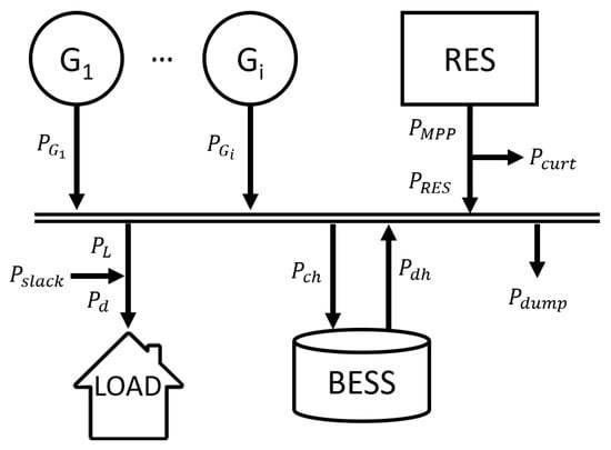
Figure 1.
Power flows in a microgrid. The designed procedure can be applied with an arbitrary number of dispatchable generators and is not affected by the nominal size of the components.
The power balance on the common bus of the single-node network, enforced at all the considered time instants, is shown in Equation (1).
The first power contribution to the microgrid () is due to the presence of an arbitrary number of dispatchable generators: their power setpoint can be fully controlled by the EMS, within their technical limits. The operating conditions of these units are defined by their minimum and maximum power and their efficiency curves, linking power production to fuel consumption in a non-linear way.
The contribution of non-programmable RES is determined starting from the forecasted generation potential profiles, i.e., the power produced at the maximum power point (). The microgrid EMS can then curtail the production from renewable sources to obtain the net power fed into the grid , as reported in Equation (2):
All the loads present in the network are modeled as a single power absorption point, characterized by an expected load profile (). The energy model used, as displayed in Equation (3), accounts for the possibility that part of the load is not covered by production. This case (which is discarded in the optimization process) is modeled using a virtual power generation , i.e., the required power from loads that is not covered by production.
The storage system can draw () energy and inject () energy into the network, based on the decisions of the EMS. Finally, the model admits the possibility of having excess power generation not absorbed by the loads (). This term is also characteristic of non-optimal solutions.
The energy storage system is defined by its nominal capacity (), its minimum and maximum states of charge (SoC) that can be achieved ( and ), and its maximum absorbable and deliverable power ( and , respectively) [33].
Finally, the battery is characterized by a charging and discharging efficiency. The operation of the battery energy storage system (BESS) is described in Equations (4) and (5) [34].
where and are the state-of-charge variations in charging and discharging, respectively, is the considered time discretization expressed in hours, and and are the charging and discharging efficiencies.
Given this microgrid model, it is possible to analyze the management variables, performance parameters, and constraints that should be taken into account in the optimization process.
3.2. Microgrid Independent Variables
The microgrid independent variables are the degrees of freedom that can be exploited by the EMS to optimize the microgrid’s operating schedule. In particular, for the presented model, they are the power produced by the dispatchable generators, the power absorbed (), and the power delivered () by the BESS.
The other powers (curtailment, slack, and dump) can be obtained from the free variables identified using the following set of rules. Specifically, they depend on the residual power between production and consumption. The expression for the net power is given by Equation (6), which shows the different terms and contributions employed for its evaluation:
If is negative, it means that the network is not able to satisfy all the demands of the loads and, consequently, there will be a slack power, as shown in Equation (7):
Conversely, if is positive, production exceeds demand. In this case, renewable generation must be curtailed or surplus energy dumped. As shown in Equations (8) and (9), in the application under analysis, the curtailment is performed first, followed by the dump:
This excess power management choice does not affect the optimization process, as the decision to perform curtailment or generation dumping does not have a substantial effect on system performance.
3.3. Constraints
Following the identification of the independent variables, the constraints considered in this study can be systematically analyzed. Notably, the power balance (Equation (1)) is intrinsically maintained through the selection of free variables and the corresponding computation of the power dissipation or slack load.
The constraints of the problem arise from both the operational requirements of the microgrid and the technical limitations of its components.
To avoid trivial solutions where all the power of the loads is slack, it is necessary to impose the first constraint. As shown in Equation (10), the slack is set to zero:
In the case that the size of dispatchable generators is adequate to cover all the loads, it is possible to always satisfy this constraint.
At this point, it is necessary to consider the constraints related to the technical limits of the microgrid components. Starting from dispatchable generators, it is possible to write the constraints on the minimum and maximum power, as shown in Equation (11):
where is the on/off status of the i-th dispatchable generator, which is given by Equation (12):
In the case of BESSs, it is necessary to consider both the constraints on the minimum and maximum states of charge and the constraints on the maximum absorbed or supplied power [34]. The set of constraints taken into account is shown in Equation (13):
The last constraint considered in this paper is the spinning reserve requirement, which requires always having an upward generation margin to compensate for potential stochastic fluctuations in loads and non-dispatchable generation [24]. Equation (14) gives the expression for the spinning reserve (). This must be provided by the dispatchable units of the microgrid (e.g., the diesel generators) and the BESS.
where is the discharging efficiency of the BESS and is the on/off status of the i-th dispatchable generator.
The required spinning reserve can be computed, based on [24], as shown in Equation (15).
where and quantify the maximum expected sudden demand increase and the PV output decrease, respectively, with respect to the forecasted values.
The formulation of the spinning reserve constraint is given by Equation (16):
All the presented constraints must be enforced at all time intervals considered; consequently, it can be seen that the optimization problem is highly constrained.
3.4. Performance Parameters
The main goal in the optimization of the microgrid EMS is to reduce operating costs. This can be achieved by minimizing the total fuel consumption. At each time step, the fuel consumption can be calculated as shown in Equation (17):
where is the power generated by the dispatchable units, is the generation efficiency at that power level, and is the on/off status of the generators.
By analyzing this equation, it can be seen that there are two ways to improve system performance: first, by reducing the power contribution from the dispatchable generators, and second, by operating them at load levels with higher efficiency. In general, both of these objectives can be achieved by efficiently managing renewable energy sources and the battery storage system.
4. Method
In this section, the proposed customization method for the evolutionary algorithm-based EMS is described. This method aims to be flexible in terms of both the microgrid model and the selected EAs. Moreover, it should provide effective results. It is based on the proper choice of optimization variables and the exploitation of heuristic constraints to reduce the problem dimensionality. Moreover, the cost function is defined to help the algorithm converge using a proper penalty for infeasible and sub-optimal solutions.
This section is structured as follows. First, the general framework of the method is proposed, and then each step is detailed.
4.1. Optimization Framework
The proposed method is designed, taking into account the selection of optimization variables, the calculation of the physical free problem variables from the optimization variables, and the cost calculation.
Through its specific operators, the optimization algorithm generates a set of candidate solutions (blue blocks in Figure 2). Each candidate solution represents a possible trajectory of the battery energy storage system (BESS) within the microgrid. Based on this information and by utilizing the microgrid model, all relevant power flows are computed, including the power exchanges of the BESS, the setpoints for the dispatchable generators, and the overall system balancing (purple blocks in Figure 2). The balancing process depends on the specific operating scenario considered (green blocks in Figure 2).
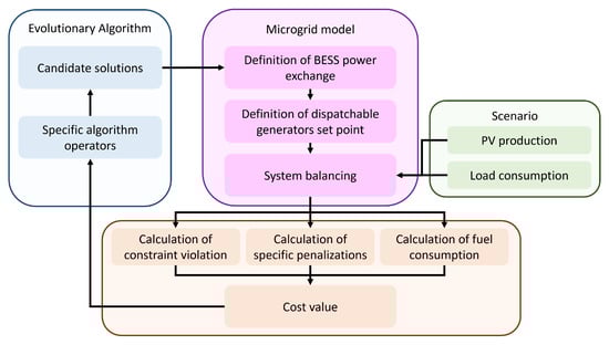
Figure 2.
Flowchart of the proposed method. The algorithm uses its operators to create candidate solutions that represent the trajectory of the BESS. The microgrid model computes the power flows that are used in the cost function to close the loop.
The computed power flows are subsequently used by the cost function module (orange blocks in Figure 2) to evaluate constraint violations, apply penalty terms, and estimate fuel consumption. The total cost value is then calculated according to Equation (32). This cost value is fed back into the optimization algorithm, which proceeds to the next iteration, based on the updated evaluations.
The proposed approach differs from the standard methodology in two main aspects. First, it involves the specific selection of optimization variables and a corresponding redefinition of the steps required to compute the power contributions within the system. These steps are designed to minimize the infeasible regions in the search space and reduce the number of optimization variables. Second, a dedicated penalty strategy is introduced to enhance the convergence of the optimization process.
4.2. Decodification of Optimization Variables
The first step in the proposed methodology is transforming the optimization variables into the power contributions to the microgrid.
The optimization variables are defined as the BESS state-of-charge values at each time step (). This value should be limited by the minimum and maximum allowable states of charge, as stated in inequality (18):
The corresponding power exchanges are derived by calculating the SoC variation, as shown in Equation (19):
The power exchanged is then constrained to remain within the BESS operational power limits, i.e., the maximum charging and discharging powers. The corresponding calculations are shown in Equations (20) and (21):
These steps are shown in Figure 3. Figure 3a shows a sample profile of the (the blue line); this is defined by the optimizer, and it naturally takes into account the minimum and maximum allowed SoCs (black horizontal lines) from the allowed ranges of the optimization variables. From the computed SoC variations, the BESS power exchanges are then calculated, as shown in Figure 3b; the power limits (black lines) are embedded in this power calculation in order to reduce the constraints that should be considered in the optimization process.

Figure 3.
Steps for defining the from the optimization variables: (a) The optimizer defines the time profile of the state of charge. (b) From the variation, the power exchanged by the BESS can be computed, also considering the power constraints.
The power exchanged by the BESS and the scenario information can be used to compute the total power required by the dispatchable generators and, consequently, the power output of each one. The calculation of the required power is performed by exploiting the power balance (Equation (1)), assuming that the slack, dumped, and curtailed power are zero. The formulation used is displayed in Equation (22):
where .
Given , the dispatchable generator outputs are determined by solving a simplified optimization problem that minimizes fuel consumption while respecting generator constraints. The definition of the optimization problem is shown in Equation (23):
In this minimization problem, the technical limits of the generators are considered. In addition, potential ramp-up and ramp-down limits can be added by properly adjusting the minimum and maximum operating powers of each generator at each time instant, based on its operating load determined in the previous timestep.
If dynamic constraints are not present, this load allocation can be precomputed and excluded from the main EMS optimization loop, reducing overall computational cost. This approach allows the proposed method to minimize the specific consumption at each time step, improving optimization convergence.
The solution of the lower-level minimization problem for the identification of the power contribution of each dispatchable generator can introduce some undesired power contributions (curtailed, dumped, and slack power). These can be calculated using Equations (6)–(9).
The final output of the algorithm is the definition of all the power terms within the microgrid. The last steps required to fully define the optimization method involve managing the constraints and defining the cost function.
4.3. Managing the Constraints and Defining the Cost Function
The proposed selection of the optimization variables allows for a drastic reduction in the number of constraints that must be considered in the optimization process. This is possible because the physical component limits are inherently satisfied.
The two constraints that must be checked are related to the slack power and the spinning reserve. Both are included in the optimization problem using a penalty approach, thus solving an unconstrained problem in which infeasible solutions incur additional cost components.
The main cost component is the total fuel consumption over the analyzed time horizon. In addition to these three cost components, two other penalties for dumped and curtailed power are introduced to improve the algorithm’s convergence.
As shown in Equation (24), the resulting cost value comprises five components:
The fuel-related cost is detailed in Equation (25):
The violation of the slack power constraint is taken into account with the cost component, as shown in Equation (26):
where is a penalty value and is the Heaviside function defined in Equation (27):
This definition of the constraint violation cost is introduced because with a proper selection of the value of (1.5 × 10³ in the analyzed problem), all infeasible solutions have a cost higher than the feasible ones. Moreover, the second penalty term (proportional to the entity of the violation) helps the algorithm converge toward solutions with a lower constraint violation.
The violation of the spinning reserve is considered using a similar approach. The missing spinning reserve can be defined as a function of the difference between the required and available ones, as shown in Equation (28):
Thus, the cost component is formulated in Equation (29):
The curtailment penalty employed, as shown in Equation (30), helps the optimization move toward the optimal solution because it reinforces the benefit of exploiting RES production:
In this cost component, the step penalty is not introduced because it prevents the correct convergence of the optimization. Moreover, the optimal value is very low ( in the analyzed test case).
Finally, the dump power penalty is managed similarly to the curtailment penalty, and its expression is shown in Equation (31):
In order to achieve proper algorithm convergence, the value should be lower than the value. In particular, in this work, it is set to using a sensitivity analysis.
Once the different terms have been defined, it is possible to present the final and comprehensive formulation of the cost function, as shown in Equation (32). In this way, the different contributions and physical properties that play a role in the objective function can be inferred.
5. Case Study
The proposed methodology was numerically tested on a case study based on the data collected from a real off-grid hybrid microgrid. The required inputs for the simulations are the load consumption profile and the PV-generation potential profile. All the data employed in the study have hourly time resolution.
The microgrid studied can be modeled as detailed in the problem formulation and is composed of two 550 kW peak diesel engines, a 1000 kWp photovoltaic system, a battery energy storage system (BESS) with a maximum capacity of 1440 kWh, and a variable non-programmable load with a maximum power absorption of 928.3 kW. The microgrid is not connected to the main electrical grid. The microgrid scheme is shown in Figure 4.
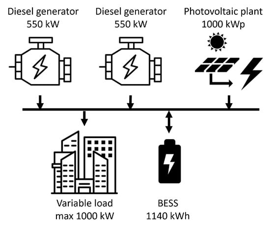
Figure 4.
Scheme of the analyzed microgrid.
Some examples of the PV power production profiles and the demand for a sample week in the year are shown in Figure 5.
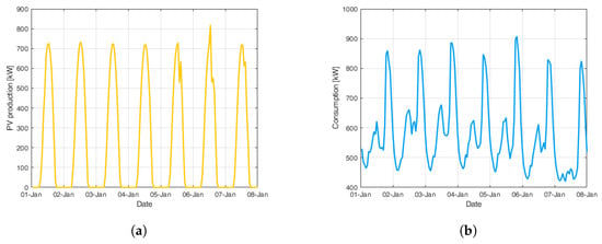
Figure 5.
Examples of (a) renewable power production and (b) load profile. These values were measured in a real microgrid.
The microgrid energy storage system has a nominal capacity () of 1440 kWh; however, a minimum state of charge (SoC) and a maximum value (1% and 90%, respectively) are considered. In terms of power, the BESS is characterized by maximum deliverable power ( kW) and absorbable power ( kW). In the case under analysis, it can be seen that these values do not constitute a particular constraint; however, they are taken into account in the design of the optimization system to ensure maximum flexibility.
The two diesel engines have a maximum power of 550 kW and a minimum power of 110 kW. Below this threshold, the engine is off ( W). Figure 6 shows the details of the consumption curves of the two generators, indicated as and in the figure. The left axis shows the consumption as a function of the produced power; the efficiency of the engines is not constant, resulting in a quadratic consumption curve. The right axis shows the specific consumption of the two engines; the reduction in the fuel consumption with the produced power shows that it is convenient to avoid using the engines with low required power.
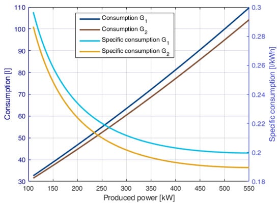
Figure 6.
Characteristics of the two engines in the microgrid: the left axis represents the consumption, and the right axis represents the specific consumption.
The optimal power breakdown between the two generators can be calculated a priori by solving the minimization problem in Equation (23). The results of the breakdown as a function of the total required power are shown in Figure 7. Figure 7a shows the power produced by each generator ( in blue and in orange). Due to the lower specific consumption of , this generator is preferentially used; in particular, if the power production is below its maximum limit, only this engine is activated. Figure 7b shows the total specific consumption of the combination of the two engines (left axis) and the best breakdown value obtained in the minimization problem (right axis). The curve of the specific consumption shows a step corresponding to the ignition of the second engine, which has a lower generation efficiency.
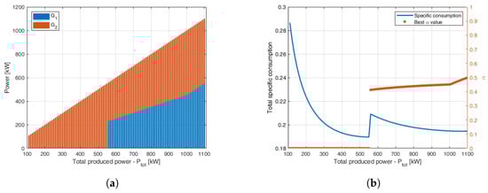
Figure 7.
Optimal power breakdown between the two dispatchable generators: (a) the proportion of power produced by the two generators as a function of the total required power; (b) the total specific consumption and the breakdown value.
6. Results
The proposed method was validated on the described case study, and this section discusses the results of the assessment.
This section is divided into three parts. In the first one, different EAs are applied with the proposed method for optimization on a sample scenario extracted from the described test case. Then, the optimal solution of the best-performing algorithm is analyzed. Finally, the proposed method is compared with a standard optimization procedure on a set of scenarios to assess the robustness of the methodology.
All the analyses were performed on an Intel(R) Core(TM) i9-10900KF 3.70 GHz. The number of objective function calls was used as the termination criterion, as it correlates with total optimization time. It also enables fair comparisons across algorithms with different population sizes. In order to ensure the statistical reliability of the results, several independent trials were performed in all the tests.
Table 1 shows an overview of the tests performed in this section, highlighting the number of cost function calls, the number of independent trials, and the number of scenarios tested.

Table 1.
Overview of the tests performed in this section.
6.1. Algorithm and Parameter Selection
To identify the most suitable evolutionary algorithm for the proposed application, a comparative analysis was conducted among five different algorithms: Social Network Optimization (SNO) [35], Differential Evolution (DE) [36], Biogeography-Based Optimization (BBO) [37], Particle Swarm Optimization (PSO), and a Genetic Algorithm (GA) [38].
Table 2 summarizes the working parameters of the algorithms employed. They represent the population size in addition to algorithm-specific parameters, such as the mutation rate for the GA and the inertia for PSO.
Table 2.
Parameters of the four tested evolutionary algorithms: (a) Social Network Optimization, (b) Genetic Algorithm, (c) Biogeography-Based Optimization, (d) Particle Swarm Optimization, and (e) the Differential Evolution.
Figure 8 presents the average convergence curves, computed over 100 independent trials, for the evaluated optimization algorithms. The results are displayed on a logarithmic scale to highlight differences in convergence behavior. PSO and the GA exhibited a very rapid initial convergence; however, their progress slowed earlier compared to the other algorithms. In terms of final performance, SNO, DE, BBO, and the GA achieved comparable results. Notably, SNO demonstrated particularly competitive behavior, maintaining superior performance over the majority of the optimization process.
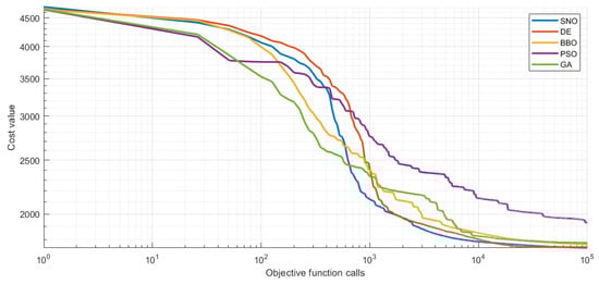
Figure 8.
Average convergence curves of all the tested algorithms.
An additional critical aspect in selecting the most appropriate algorithm for EMS applications is the robustness of the optimization process. Figure 9 shows box plots of the results obtained from 100 independent trials for each algorithm. This analysis highlights the strong performance of SNO and DE, which demonstrated not only excellent convergence capabilities but also high consistency across trials, indicating the greater reliability of the solutions produced.
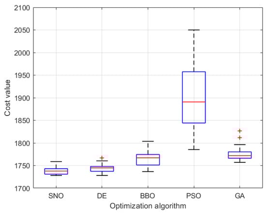
Figure 9.
Box plot for statistical assessment of the tested algorithms. The red plus signs represent the outliers.
Finally, since in operation, computational time is very important, Table 3 shows the average computational time required by each of the tested algorithms. Performance was comparable across all the algorithms, and the optimization times were compatible with the specific EMS application. In fact, due to the changing conditions of the loads and weather, it was often necessary to run the optimization several times.
Table 3.
Computational time required for the optimization in seconds.
From the comparison, the superior performance of the DE and SNO algorithms emerged compared to PSO, the GA, and BBO. Particularly notable was their much higher reliability, inferable from the considerably lower standard deviation values achieved. Therefore, for the application analyzed here, they have more robust optimization capabilities compared to the other three methods. Focusing on the SNO and DE algorithms, Figure 9 shows that SNO achieved both a slightly lower mean value and standard deviation. Therefore, to optimize the current problem, the Social Network Optimization algorithm was selected, and its optimization process and working principles are briefly reported in the next section.
The cost function presented in Equation (32) includes scalarization parameters. Their values were selected based on a sensitivity analysis conducted using the SNO algorithm. The results of this analysis are shown in Figure 10. While the introduction of these parameters led to a slight improvement in the overall performance of the algorithm, the most significant effect was a noticeable reduction in the dispersion of the results, thereby enhancing the robustness of the optimization process.
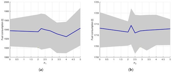
Figure 10.
Sensitivity analysis of the penalty coefficients and , respectively in (a) and (b): the blue line represents the average fuel consumption, while the gray bands show the dispersion of the results.
6.2. Analysis of SNO Optimization Process
The SNO algorithm is a population-based evolutionary algorithm. It is inspired by the dynamics of social media platforms and the way information circulates within them. In this algorithm, the pool of potential solutions represents users in a virtual social network, imitating how individuals communicate, exchange ideas, and engage with one another online. Given its superior performance, it was selected for the optimization study, and its optimization process was analyzed in more detail.
Figure 11 shows the convergence curves of 50 independent trials of SNO; each trial is represented by a thin gray line, and the thick blue line represents the average convergence. Due to the wide variation in cost values in the optimization, an insert zooms in on the lower cost values. Finally, the histogram on the right of the figure shows the distribution of the final values of each trial.

Figure 11.
Convergence curves of 50 independent trials of SNO on an optimization scenario. Each gray line represents one trial, while the thick line represents the average convergence. The insert zooms in on lower cost values, while the histogram on the right shows the distribution of the final values.
Analyzing the convergence, a sharp drop can be seen in the early stages of the process, which corresponds to the fulfillment of the constraints, particularly the spinning reserve requirement. Then, the convergence rate decreases because the optimization process enters the exploitation phase to improve the solution quality.
The distribution of the final values is concentrated on low costs, even if some trials do not properly converge. This is due to the intrinsic stochastic nature of evolutionary algorithms. However, the low dispersion indicates good algorithm reliability; thus, only a few independent trials are required in real applications of this approach.
Figure 12 shows the optimal solution found by SNO for the analyzed scenario. Figure 12a represents the power flows in the microgrid; the red line represents the total demand, while the bars represent all the power contributions. The EMS utilizes the first part of the day to charge the battery, drawing energy from both the dispatchable generators and the photovoltaic production. This evolution is evident in Figure 12b, which shows the evolution over time of the state of charge; each scenario analyzed starts with the BESS at its minimum value. Since the remaining energy content in the storage is not in the cost function, the final SoC in the optimal solution is the minimum allowed.
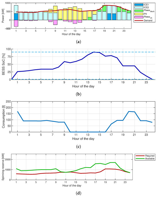
Figure 12.
Optimal solution found by SNO: (a) Energy flow in each hour of the day; (b) Evolution of the BESS SoC; (c) Consumption in each hour; (d) Spinning reserve.
Figure 12c shows the total consumption of the two dispatchable generators. The main cost component minimized is the integral of this curve.
Finally, Figure 12d shows the available and required spinning reserves, where the red line represents the required reserve and the green line represents the actual reserve. Analyzing these curves, it is clear that this constraint affects the optimal solution because the algorithm cannot turn off the ICEs earlier; otherwise, the available spinning reserve would become too low.
In the next subsection, the proposed approach is compared with a standard optimization method across several scenarios.
6.3. Comparison with Standard Approach
After analyzing the optimization process using the proposed problem codification and SNO method, the method was compared with a standard approach. Using the standard approach, an optimization process is considered here in which all the free problem variables (power production of dispatchable generators and SoC trajectory of the BESS) are directly managed by the optimizer. This standard approach is referred to in the following as full optimization.
The comparison was conducted across 28 different scenarios, optimizing with SNO and performing 50 independent trials. Using diverse scenarios demonstrates the approach’s robustness to variations in loads and RES production.
Figure 13 shows a comparison in terms of the consumption of the final solution. Each bar represents the average value, and the 5th and the 95th percentiles are represented by the black whiskers. The green bars represent the analyzed methodology, and the orange ones represent full optimization. The figure shows the superiority of the proposed approach in terms of both the average value and standard deviation across all the analyzed scenarios in absolute terms. In this way, the actual advantages in terms of fuel consumption when the microgrid is managed with the optimization method proposed are highlighted. In addition, it is possible to compare the two methods also in relative terms. On average, compared to a standard scheduling approach, our optimization methodology leads to an improvement of 11.87%. Therefore, the proposed approach shows a significant reduction in fuel consumption in both absolute and relative terms.
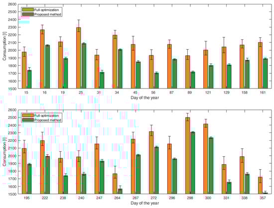
Figure 13.
Comparison between full optimization and the proposed approach across 28 different scenarios. The bars represent the average values of 50 independent trials, and the black whiskers represent the 5th and the 95th percentiles.
The advantages of the proposed method can also be analyzed using the convergence curves for one of the sample scenarios, as shown in Figure 14, which highlights that both the final value and reliability improved with the proposed approach. Indeed, in this case, the average value obtained by the 50 independent trials is lower, and the confidence band is thinner.
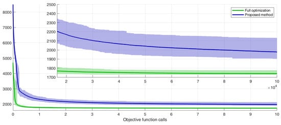
Figure 14.
Comparison of the convergence curves of the proposed method (in green) and full optimization (in purple). The thick lines represent the average value of 50 independent trials, and the shaded area represents the 98% confidence band.
In order to identify where the improvement in performance is introduced and the proposed approach’s reliability lies, the cost contributions were analyzed for all the scenarios, as shown in Figure 15. In particular, the figure shows how the variation in the final fuel consumption was obtained; all the bars are positive because the consumptions obtained by the proposed method were lower than those found by the standard approach. Each bar is divided into two parts: blue represents the amount of fuel saved by reducing the power production of the diesel engine, and brown represents the fuel saved using a better selection of the working point of the generators at the same value of power output.
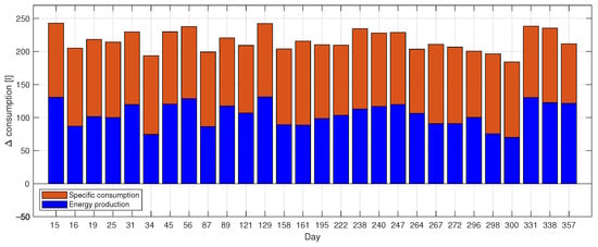
Figure 15.
Components of the variation in fuel consumption between the proposed method and full optimization: blue represents the fuel saved by the proposed approach due to lower energy consumption, while brown represents the fuel saved due to better specific consumption.
These results show that the improvement is, on average, driven by lower energy production. This is due to the reduced number of optimization variables and the introduction of the energy balance in the variable decodification process. The remaining improvement is due to better specific consumption, which is due to the separate minimization problem used to define the diesel generators’ power breakdown.
6.4. Improved Storage Energy Management
The implemented Energy Management System improves storage management by addressing two key factors: reducing energy losses in the BESS and minimizing the number of charge-discharge cycles.
The energy losses are primarily determined by the BESS’s efficiency, and the optimization algorithm identifies a solution that operates at the maximum efficiency point. Figure 16 shows this improvement, with the data normalized to the total daily energy demand.
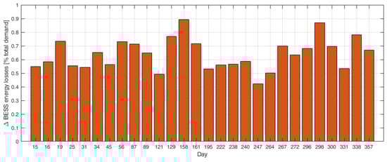
Figure 16.
Difference in energy losses between basic optimization and the proposed method. The data are normalized with respect to the total daily energy demand.
The degradation of the battery can be analyzed by computing the number of cycles performed by the battery on each of the tested days. Figure 17 shows the comparison between the basic optimization and the proposed method on the number of battery cycles. The results take into account 50 independent trials. The bars represent the average values, and the whiskers the 5th and the 95th percentiles.

Figure 17.
Comparison of the number of battery cycles between full optimization and the proposed approach across 28 different scenarios. The bars represent the average values of 50 independent trials, and the black whiskers represent the 5th and the 95th percentiles.
The results show that the proposed method is able to reduce the average number of cycles per day from 1.42 to 0.92, corresponding to an improvement of 35%.
7. Conclusions
In this paper, evolutionary algorithms were applied to optimize scheduling decisions in the Energy Management System of a microgrid. The proposed approach is capable of finding the optimal trade-off between the degrees of freedom of the optimization algorithm and the heuristic information introduced in the optimization process. The proposed approach was tested with different evolutionary algorithms, and Social Network Optimization achieved the best performance. This procedure was compared with a traditional approach in which the optimization algorithm can tune all of the free design variables. The results show that the heuristic information introduced is very important for the quality of the final result. In addition, the proposed method enhances battery management by accounting for both energy losses and battery degradation.
The results obtained in this work can serve as a benchmark for the application of reinforcement learning. These approaches are particularly promising, as they can be implemented in real time and are inherently more robust to the uncertainties associated with loads and weather forecasting. However, their deployment requires a dedicated training phase for each new microgrid configuration, which can be a limiting factor. Furthermore, RL methods are highly data-intensive, necessitating the availability of large and representative datasets to achieve satisfactory performance.
Author Contributions
Conceptualization, A.N., A.G. and S.L.; Data curation, A.N., L.F.B. and S.T.; Formal analysis, R.Z. and S.L.; Investigation, A.N. and S.T.; Methodology, A.G. and R.Z.; Project administration, S.L. and F.G.; Resources, A.N. and F.G.; Software, S.T. and L.F.B.; Supervision, A.G. and S.L.; Validation, L.F.B. and R.Z.; Visualization, A.N. and F.G.; Writing—review and editing, A.N. and S.T. All authors have read and agreed to the published version of the manuscript.
Funding
This study was carried out within MOST (The National Center for Sustainable Mobility) and received funding from the European Union’s Next-GenerationEU (PIANO NAZIONALE DI RIPRESA E RESILIENZA (PNRR)—MISSIONE 4 COMPONENTE 2, INVESTIMENTO 1.4—D.D. 1033 17/06/2022, CN00000023). This manuscript reflects only the authors’ views and opinions; neither the European Union nor the European Commission can be considered responsible for them. This work was supported by the Italian Ministry for Education, University, and Research under the project PRIN2022 “BERENICE - Battery energy management systems for renewable and citizen energy communities”, identified by reference number P2022R3L83, which is part of the National Recovery and Resilience Plan (PNRR).
Data Availability Statement
The data presented in this study are available on request from the corresponding author due to privacy concerns about electricity consumption data.
Conflicts of Interest
The authors declare no conflicts of interest.
Abbreviations
The following abbreviations are used in this manuscript:
| BBO | Biogeography-Based Optimization |
| BESS | Battery Energy Storage System |
| CI | Computational Intelligence |
| DE | Differential Evolution |
| EA | Evolutionary Algorithm |
| EMS | Energy Management System |
| EV | Electric Vehicle |
| FIS | Fuzzy Inference System |
| GA | Genetic Algorithm |
| MILP | Mixed-Integer Linear Programming |
| PSO | Particle Swarm Optimization |
| RES | Renewable Energy Sources |
| SoC | State of Charge |
| SNO | Social Network Optimization |
| List of Symbols | |
| Power production of the i-th dispatchable generator | |
| Maximum power produced by RES | |
| Effective power input from RES | |
| Curtailed power from RES | |
| Total load power absorption | |
| Load slack power | |
| Effective load power absorption | |
| BESS charging power | |
| BESS discharging power | |
| Dumped power | |
| BESS nominal capacity | |
| / | BESS maximum charging/discharging power |
| / | BESS SoC variation in charge/discharge |
| Time discretization interval | |
| / | BESS charging/discharging efficiency |
| Fuel consumption of the i-th dispatchable generator | |
| Efficiency of the i-th dispatchable generator at power | |
| / | Minimum/maximum power of the i-th dispatchable generator |
| BESS minimum state of charge | |
| BESS maximum state of charge | |
| Available spinning reserve | |
| On/off status of the i-th dispatchable generator |
References
- Zidane, T.E.K.; Ab Muis, Z.; Ho, W.S.; Zahraoui, Y.; Aziz, A.S.; Su, C.L.; Mekhilef, S.; Campana, P.E. Power systems and microgrids resilience enhancement strategies: A review. Renew. Sustain. Energy Rev. 2025, 207, 114953. [Google Scholar] [CrossRef]
- Gholami, M.; Muyeen, S.; Mousavi, S.A. Optimal sizing of battery energy storage systems and reliability analysis under diverse regulatory frameworks in microgrids. Energy Strategy Rev. 2024, 51, 101255. [Google Scholar] [CrossRef]
- Bhatia, A.A.; Das, D. Demand response strategy for microgrid energy management integrating electric vehicles, battery energy storage system, and distributed generators considering uncertainties. Sustain. Energy Grids Netw. 2025, 41, 101594. [Google Scholar] [CrossRef]
- Ali, L.; Azim, M.I.; Peters, J.; Bhandari, V.; Menon, A.; Tiwari, V.; Green, J.; Muyeen, S. Application of a community battery-integrated microgrid in a blockchain-based local energy market accommodating P2P trading. IEEE Access 2023, 11, 29635–29649. [Google Scholar] [CrossRef]
- Micallef, A.; Guerrero, J.M.; Vasquez, J.C. New horizons for microgrids: From rural electrification to space applications. Energies 2023, 16, 1966. [Google Scholar] [CrossRef]
- Eyimaya, S.E.; Altin, N. Review of Energy Management Systems in Microgrids. Appl. Sci. 2024, 14, 1249. [Google Scholar] [CrossRef]
- Thirunavukkarasu, G.S.; Seyedmahmoudian, M.; Jamei, E.; Horan, B.; Mekhilef, S.; Stojcevski, A. Role of optimization techniques in microgrid energy management systems—A review. Energy Strategy Rev. 2022, 43, 100899. [Google Scholar] [CrossRef]
- Alghamdi, A.S. Microgrid energy management and scheduling utilizing energy storage and exchange incorporating improved gradient-based optimizer. J. Energy Storage 2024, 97, 112775. [Google Scholar] [CrossRef]
- Bilal, M.; Algethami, A.A.; Hameed, S. Review of computational intelligence approaches for microgrid energy management. IEEE Access 2024, 12, 123294–123321. [Google Scholar] [CrossRef]
- Nespoli, A.; Ogliari, E.; Pretto, S.; Gavazzeni, M.; Vigani, S.; Paccanelli, F. Electrical Load Forecast by Means of LSTM: The Impact of Data Quality. Forecasting 2021, 3, 91–101. [Google Scholar] [CrossRef]
- Niccolai, A.; Dolara, A.; Ogliari, E. Hybrid PV Power Forecasting Methods: A Comparison of Different Approaches. Energies 2021, 14, 451. [Google Scholar] [CrossRef]
- Gharehveran, S.S.; Shirini, K.; Khavar, S.C.; Mousavi, S.H.; Abdolahi, A. Deep learning-based demand response for short-term operation of renewable-based microgrids. J. Supercomput. 2024, 80, 26002–26035. [Google Scholar] [CrossRef]
- Jumani, T.A.; Mustafa, M.W.; Alghamdi, A.S.; Rasid, M.M.; Alamgir, A.; Awan, A.B. Swarm intelligence-based optimization techniques for dynamic response and power quality enhancement of AC microgrids: A comprehensive review. IEEE Access 2020, 8, 75986–76001. [Google Scholar] [CrossRef]
- Ahmad, S.; Shafiullah, M.; Ahmed, C.B.; Alowaifeer, M. A review of microgrid energy management and control strategies. IEEE Access 2023, 11, 21729–21757. [Google Scholar] [CrossRef]
- Papazoglou, G.; Biskas, P. Review and comparison of genetic algorithm and particle swarm optimization in the optimal power flow problem. Energies 2023, 16, 1152. [Google Scholar] [CrossRef]
- Mohapatra, P.; Roy, S.; Das, K.N.; Dutta, S.; Raju, M.S.S. A review of evolutionary algorithms in solving large scale benchmark optimisation problems. Int. J. Math. Oper. Res. 2022, 21, 104–126. [Google Scholar] [CrossRef]
- Piotrowski, A.P.; Napiorkowski, J.J.; Piotrowska, A.E. Particle swarm optimization or differential evolution—A comparison. Eng. Appl. Artif. Intell. 2023, 121, 106008. [Google Scholar] [CrossRef]
- Pradhan, P.C.; Sahu, R.K.; Panda, S. Comparative performance analysis of hybrid differential evolution and pattern search technique for frequency control of the electric power system. J. Electr. Syst. Inf. Technol. 2021, 8, 1–21. [Google Scholar] [CrossRef]
- Moretti, L.; Meraldi, L.; Niccolai, A.; Manzolini, G.; Leva, S. An Innovative Tunable Rule-Based Strategy for the Predictive Management of Hybrid Microgrids. Electronics 2021, 10, 1162. [Google Scholar] [CrossRef]
- Zhang, Q.; Wei, L.; Yang, B. Research on Improved BBO Algorithm and Its Application in Optimal Scheduling of Micro-Grid. Mathematics 2022, 10, 2998. [Google Scholar] [CrossRef]
- Ahmethodžić, L.; Musić, M.; Huseinbegović, S. Microgrid energy management: Classification, review and challenges. CSEE J. Power Energy Syst. 2022, 9, 1425–1438. [Google Scholar]
- Sun, C.; Joos, G.; Ali, S.Q.; Paquin, J.N.; Rangel, C.M.; Al Jajeh, F.; Novickij, I.; Bouffard, F. Design and real-time implementation of a centralized microgrid control system with rule-based dispatch and seamless transition function. IEEE Trans. Ind. Appl. 2020, 56, 3168–3177. [Google Scholar] [CrossRef]
- Kassab, F.A.; Celik, B.; Locment, F.; Sechilariu, M.; Liaquat, S.; Hansen, T.M. Optimal sizing and energy management of a microgrid: A joint MILP approach for minimization of energy cost and carbon emission. Renew. Energy 2024, 224, 120186. [Google Scholar] [CrossRef]
- Moretti, L.; Polimeni, S.; Meraldi, L.; Raboni, P.; Leva, S.; Manzolini, G. Assessing the impact of a two-layer predictive dispatch algorithm on design and operation of off-grid hybrid microgrids. Renew. Energy 2019, 143, 1439–1453. [Google Scholar] [CrossRef]
- Zhu, X.; Ruan, G.; Geng, H.; Liu, H.; Bai, M.; Peng, C. Multi-objective sizing optimization method of microgrid considering cost and carbon emissions. IEEE Trans. Ind. Appl. 2024, 60, 5565–5576. [Google Scholar] [CrossRef]
- Capillo, A.; De Santis, E.; Mascioli, F.M.F.; Rizzi, A. An Online Hierarchical Energy Management System for Energy Communities, Complying with the Current Technical Legislation Framework. arXiv 2024, arXiv:2402.01688. [Google Scholar]
- Leonori, S.; Paschero, M.; Mascioli, F.M.F.; Rizzi, A. Optimization strategies for Microgrid energy management systems by Genetic Algorithms. Appl. Soft Comput. 2020, 86, 105903. [Google Scholar] [CrossRef]
- Leonori, S.; Martino, A.; Mascioli, F.M.F.; Rizzi, A. Microgrid energy management systems design by computational intelligence techniques. Appl. Energy 2020, 277, 115524. [Google Scholar] [CrossRef]
- Gholami, K.; Dehnavi, E. A modified particle swarm optimization algorithm for scheduling renewable generation in a micro-grid under load uncertainty. Appl. Soft Comput. 2019, 78, 496–514. [Google Scholar] [CrossRef]
- Bandopadhyay, J.; Roy, P.K. Application of hybrid multi-objective moth flame optimization technique for optimal performance of hybrid micro-grid system. Appl. Soft Comput. 2020, 95, 106487. [Google Scholar] [CrossRef]
- Mazzola, S.; Vergara, C.; Astolfi, M.; Li, V.; Perez-Arriaga, I.; Macchi, E. Assessing the value of forecast-based dispatch in the operation of off-grid rural microgrids. Renew. Energy 2017, 108, 116–125. [Google Scholar] [CrossRef]
- Moretti, L.; Astolfi, M.; Vergara, C.; Macchi, E.; Pérez-Arriaga, J.I.; Manzolini, G. A design and dispatch optimization algorithm based on mixed integer linear programming for rural electrification. Appl. Energy 2019, 233, 1104–1121. [Google Scholar] [CrossRef]
- Farakhor, A.; Wu, D.; Wang, Y.; Fang, H. A novel modular, reconfigurable battery energy storage system: Design, control, and experimentation. IEEE Trans. Transp. Electrif. 2022, 9, 2878–2890. [Google Scholar] [CrossRef]
- Zheng, N.; Qin, X.; Wu, D.; Murtaugh, G.; Xu, B. Energy storage state-of-charge market model. IEEE Trans. Energy Mark. Policy Regul. 2023, 1, 11–22. [Google Scholar] [CrossRef]
- Niccolai, A.; Grimaccia, F.; Mussetta, M.; Gandelli, A.; Zich, R. Social network optimization for WSN routing: Analysis on problem codification techniques. Mathematics 2020, 8, 583. [Google Scholar] [CrossRef]
- Li, M.; Zhang, D.; Lu, S.; Tang, X.; Phung, T. Differential evolution-based overcurrent protection for DC microgrids. Energies 2021, 14, 5026. [Google Scholar] [CrossRef]
- de Oliveira-Assis, L.; García-Trivino, P.; Soares-Ramos, E.P.; Sarrias-Mena, R.; García-Vázquez, C.A.; Ugalde-Loo, C.E.; Fernández-Ramírez, L.M. Optimal energy management system using biogeography based optimization for grid-connected MVDC microgrid with photovoltaic, hydrogen system, electric vehicles and Z-source converters. Energy Convers. Manag. 2021, 248, 114808. [Google Scholar] [CrossRef]
- Firdouse, F.; Surender Reddy, M. A hybrid energy storage system using GA and PSO for an islanded microgrid applications. Energy Storage 2023, 5, e460. [Google Scholar] [CrossRef]
Disclaimer/Publisher’s Note: The statements, opinions and data contained in all publications are solely those of the individual author(s) and contributor(s) and not of MDPI and/or the editor(s). MDPI and/or the editor(s) disclaim responsibility for any injury to people or property resulting from any ideas, methods, instructions or products referred to in the content. |
© 2025 by the authors. Licensee MDPI, Basel, Switzerland. This article is an open access article distributed under the terms and conditions of the Creative Commons Attribution (CC BY) license (https://creativecommons.org/licenses/by/4.0/).