Improving Transformer Health Index Prediction Performance Using Machine Learning Algorithms with a Synthetic Minority Oversampling Technique

Putra, Muhammad Akmal A.; Suwarno,; Prasojo, Rahman Azis

doi:10.3390/en18092364

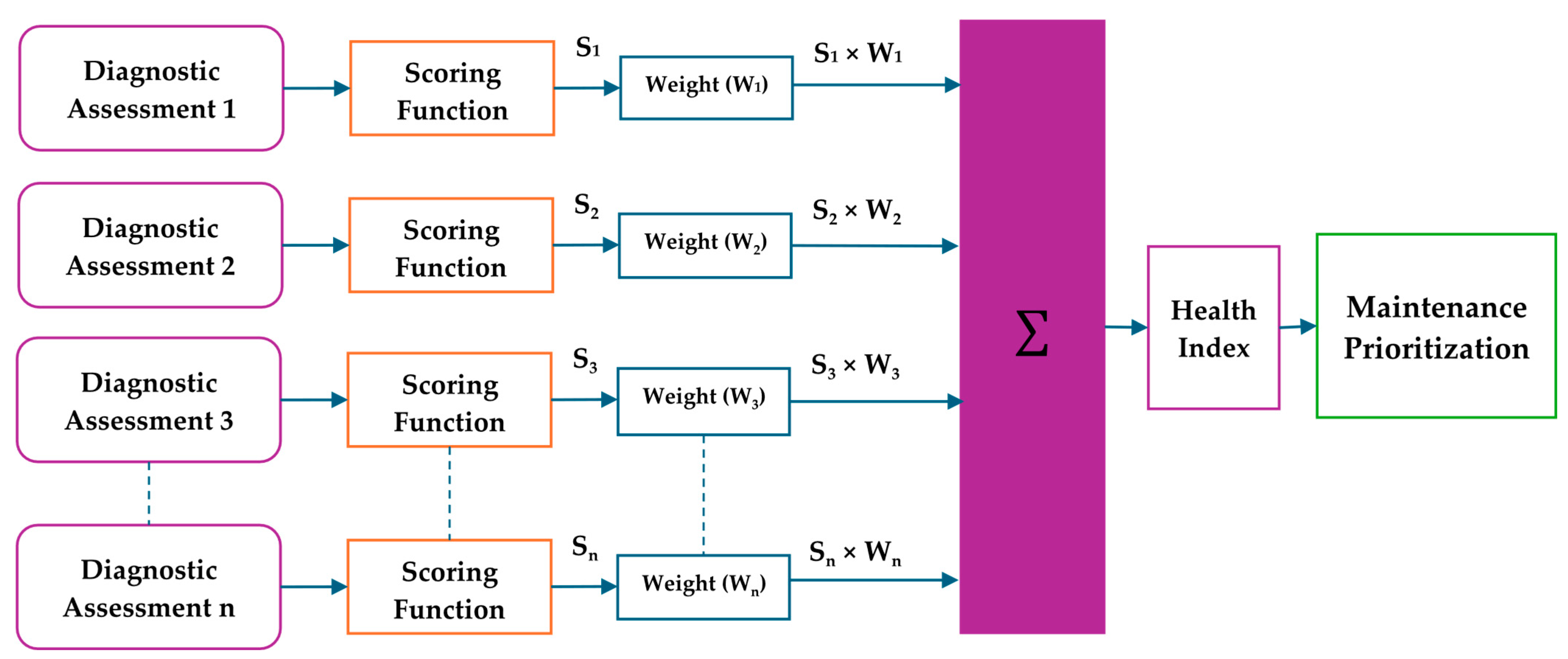
Open AccessArticle

Improving Transformer Health Index Prediction Performance Using Machine Learning Algorithms with a Synthetic Minority Oversampling Technique

by

Muhammad Akmal A. Putra

^1,*

,

Suwarno

¹

and

Rahman Azis Prasojo

²

¹

School of Electrical Engineering and Informatics, Institut Teknologi Bandung, Bandung 40132, Indonesia

²

Department of Electrical Engineering, Politeknik Negeri Malang, Malang 65141, Indonesia

^*

Author to whom correspondence should be addressed.

Energies 2025, 18(9), 2364; https://doi.org/10.3390/en18092364

Submission received: 30 March 2025 / Revised: 22 April 2025 / Accepted: 1 May 2025 / Published: 6 May 2025

(This article belongs to the Special Issue Dielectric Insulation in Medium- and High-Voltage Power Equipment—Degradation and Failure Mechanism, Diagnostics, and Electrical Parameters Improvement: 2nd Edition)

Download

Browse Figures

Versions Notes

Abstract

:

Machine learning (ML) has emerged as a powerful tool in transformer condition assessment, enabling more accurate diagnostics by leveraging historical test data. However, imbalanced datasets, often characterized by limited samples in poor transformer conditions, pose significant challenges to model performance. This study investigates the application of oversampling techniques to enhance ML model accuracy in predicting the Health Index of transformers. A dataset comprising 3850 transformer tests collected from utilities across Indonesia was used. Key parameters, including oil quality, dissolved gas analysis, and paper condition factors, were employed as inputs for ML modeling. To address the class imbalance, various oversampling methods, such as the Synthetic Minority Oversampling Technique (SMOTE), Borderline-SMOTE, SMOTE-Tomek, and SMOTE-ENN, were implemented and compared. This study explores the impact of these techniques on model performance, focusing on classification accuracy, precision, recall, and F1-score. The results reveal that all SMOTE-based methods improved model performance, with SMOTE-ENN yielding the best outcomes. It significantly reduced classification errors, particularly for minority classes, ensuring better predictive reliability. These findings underscore the importance of advanced oversampling techniques in improving transformer diagnostics. By effectively addressing the challenges posed by imbalanced datasets, this research provides a robust framework for applying ML in transformer condition monitoring and other domains with similar data constraints.

Keywords:

transformer diagnostics; Health Index; machine learning; imbalance dataset; condition assessment; Synthetic Minority Oversampling Technique

1. Introduction

High-voltage power transformers are critical and expensive components in electrical transmission lines. Power transformers play a vital role in facilitating power transmission across systems with different voltage levels. To ensure the reliability and safety of the electrical grid, the continuous monitoring and maintenance of power transformers is essential [1,2]. Effective maintenance can be achieved by evaluating specific diagnostic parameters and integrating them into a single index, known as the Health Index (HI) [3,4].

The utilization of the Health Index (HI) for power transformers has proven to be an effective tool for integrating multiple diagnostic parameters into a single comprehensive assessment. These parameters are derived from laboratory tests, which encompass three main tests. The first test is the Dissolved Gas Analysis (DGA), which evaluates seven key gases: hydrogen (H₂), methane (CH₄), acetylene (C₂H₂), ethylene (C₂H₄), ethane (C₂H₆), carbon dioxide (CO₂), and carbon monoxide (CO) [5]. The second test is Oil Quality, which includes six transformer oil factors: Breakdown Voltage (BDV), Interfacial Tension (IFT), color, humidity, Dissipation Factor (DF), and acidity. The third test is the Degree of Polymerization (DP), which involves furan testing. These three tests are combined and analyzed to determine the Health Index (HI) of the power transformer. The HI value serves as a critical input for planning routine maintenance and estimating the service life of power transformers [6,7].

Several studies have been conducted to develop conventional Health Index (HI) methods. Many of these studies utilize the scoring–weighting approach, which relies on expert judgment to determine the weight values used in the calculations. For instance, Ref. [4] employed DGA testing, loading history, power factor, and infrared testing as parameters with the highest weights. Ref. [8] prioritized DGA, oil quality, furan, dielectric loss, absorption ratio, DC resistance, and partial discharge tests, assigning higher weights to these parameters compared to loading factors. Ref. [9] combined 24 parameters with a weighting ratio of 0.4 for the tap changer and 0.6 for transformer testing. Similarly, Ref. [10] incorporated a combination of DGA, oil quality, and paper condition, with the highest weight assigned to furan testing. The scoring–weighting method has become the most widely used conventional approach for HI calculation. However, it is heavily dependent on expert judgment, which can vary significantly between utilities, potentially affecting the consistency and reliability of the results.

To address the subjectivity inherent in expert assessments, many studies have developed methods for predicting the Health Index using machine learning or artificial intelligence algorithms. Studies [11,12,13,14] developed Neural Network-based models for predicting the Health Index. Reference [15] employed a support vector machine to facilitate the computational process of calculating the Health Index, while [16,17] utilized the Random Forest algorithm to predict missing data in transformer testing parameters. Additionally, Ref. [18] developed a model for predicting transformer asset age and condition using fuzzy logic.

The implementation of machine learning can enhance the accuracy of transformer condition predictions. However, incomplete datasets obtained from the field and the limited number of transformers with poor conditions often lead to data imbalance, which reduces the performance of machine learning models [19,20]. To address the issue of imbalanced data, several studies have employed oversampling techniques to balance the dataset. Study [21] utilized the SMOTE (Synthetic Minority Oversampling Technique) method to balance DGA testing datasets and improve transformer failure diagnosis performance using MLP (Multi-Layer Perceptron). Reference [22] implemented SMOTE in a Random Forest model based on the Duval Pentagon. Additionally, References [23,24] demonstrated significant improvements in machine learning model performance when developed using SMOTE datasets.

Previous studies have demonstrated that SMOTE can enhance the performance of machine learning (ML) models. However, its application to datasets used for Health Index (HI) calculations remains underexplored, particularly for transformers in poor condition. While existing studies have shown improvements in model performance, several critical gaps persist. Firstly, previous research has often overlooked the introduction of noise caused by synthetic data generation, which can lead to the decreased reliability of predictions. Secondly, the risk of overfitting, especially when using large volumes of synthetic data, has not been adequately addressed, limiting the generalizability of these models. Thirdly, the effect of significant changes in dataset composition due to oversampling on overall model performance has not been thoroughly investigated. These challenges hinder the practical application of oversampling methods in real-world scenarios. This study aims to fill these gaps by systematically evaluating the performance of ML algorithms for predicting the Health Index while incorporating advanced oversampling techniques, such as SMOTE, Borderline-SMOTE, SMOTE-Tomek, and SMOTE-ENN. Using a dataset comprising 3850 transformer test samples collected from electrical utilities in Indonesia, this research offers a comprehensive analysis of the trade-offs between improved model accuracy and potential drawbacks, such as noise and overfitting, thereby providing valuable insights for transformer diagnostics and other domains facing similar data challenges.

2. Health Index Predictions

2.1. Transformer Data

This section presents the datasets utilized for assessing the Health Index (HI) of power transformers. The data are categorized into three main factors, namely the Oil Quality Factor, Fault Factor, and Paper Condition Factor, which collectively encompass a comprehensive set of diagnostic parameters. These datasets form the foundation for understanding transformer conditions and predicting their health categories.

The Oil Quality Factor consists of parameters derived from various oil quality tests. These include the following:

Breakdown Voltage (BDV): Breakdown voltage is a measure of the dielectric strength of transformer oil or its resistance to electrical stress. Contaminants such as water and sediment can reduce the breakdown voltage. The BDV test is conducted according to IEC standards with a 2.5 mm electrode gap.
Water content: The water content in oil influences the breakdown voltage and the aging process of both the oil and the paper insulation within the power transformer.
Acidity (Acid): Acidity, also referred to as the neutralization value, measures the level of acidity or contamination in the oil. Transformer oil acidity is formed by acidic oxidation products.
Interfacial Tension (IFT): The IFT test measures the tension between oil and water to detect the presence of polar contaminants from the degradation process. A declining IFT value indicates aging in the insulating oil. Additionally, IFT can signal problems with the interaction between the oil and other insulating materials or contamination issues during oil handling.
Color scale: The color of transformer oil changes with aging, influenced by impurities such as carbon. The test compares the color of used oil to new oil.

The Fault Factor focuses on the evaluation of dissolved gases using a Dissolved Gas Analysis (DGA). This factor comprises levels of key hydrocarbon gases such as Hydrogen (H₂), Methane (CH₄), Acetylene (C₂H₂), Ethylene (C₂H₄), and Ethane (C₂H₆).

The Paper Condition Factor provides insights into the aging and degradation of paper insulation in transformers. This factor includes the following:

Carbon Monoxide (CO) and Carbon Dioxide (CO₂): The levels of CO and CO₂ dissolved in the oil can correlate with the degree of polymerization and the tensile strength of the paper insulation. However, smaller amounts of CO and CO₂ can also result from the thermal degradation of oil, paint layers, varnishes, and phenolic resins used in transformer components. Additionally, atmospheric contamination can contribute to CO₂ levels, particularly in open configurations that allow for air circulation.
Operational age: The transformer’s operational age is often used as an indicator of the condition of the paper insulation. It is assumed that older transformers experience more operational stress and irreversible degradation.
Degree of Polymerization (DP): Solid cellulose-based insulation not only serves as a dielectric, but also provides mechanical strength, for instance, during short-circuit stress. The mechanical strength of the paper is highly correlated with the cellulose molecular chain length, indicated by the DP value. Over time, cellulose molecules break down through chain scission, reducing the DP value and mechanical strength. For new cellulose material, the DP value is approximately 1200, while for new transformers, the DP value is slightly lower due to high-temperature drying processes.

Table 1 summarizes the statistical data for the parameters collected across a population of transformers, highlighting the sample size (N), mean, minimum, first quartile (Q1), median, third quartile (Q3), and maximum values for each parameter. These statistics provide an overview of the variability and distribution of the diagnostic parameters used in this study.

2.2. Health Index Predictions Using Scoring–Weighting

Several studies have aggregated test parameters into a single Health Index (HI) value. Typically, the HI calculation employs a conventional approach that assigns a score to each parameter and multiplies it by a weight reflecting the parameter’s importance in assessing the transformer’s condition. Table 2 shows several developments in the scoring–weighting method in aggregating test parameters into Health Index values.

Figure 1 illustrates a schematic for the Health Index using the scoring-weighting method. This method normalizes the results of transformer diagnostic tests into scores, which are then multiplied by weights assigned to each test. The resulting of products then aggregated into a single value as the Health Index. The Health Index value is used to determine the maintenance priority for the transformer.

The scoring–weighting method is the most widely used approach by utilities for assessing transformer condition. However, its implementation requires assigning weight values to each parameter, with these weights determined by experts. Since experts at different utilities may assign different values, the inherent subjectivity can affect the accuracy of the transformer condition assessment, representing a significant limitation of this method.

2.3. Non-Conventional Method for Health Index Prediction

In this study, machine learning algorithms are employed to predict the Health Index (HI) of power transformers, leveraging diverse datasets from transformer testing. These methods offer significant advantages over traditional approaches by reducing subjectivity, adapting to new data, and enabling more accurate and comprehensive diagnostics [26,27,28]. The input data used in the model incorporates key transformer testing parameters categorized into three main factors: Oil Quality, Dissolved Gas Analysis (DGA), and Paper Condition [29]. Each factor comprises specific testing parameters, as follows:

Oil Quality factors:

Breakdown Voltage (BDV);
Water content;
Acidity;
Interfacial Tension (IFT);
Color scale.

Dissolved Gas Analysis (DGA):

Concentrations of Hydrogen (H₂), Methane (CH₄), Acetylene (C₂H₂), Ethylene (C₂H₄), and Ethane (C₂H₆).

Paper condition factors:

Age of transformer insulation;
Carbon Monoxide (CO) and Carbon Dioxide (CO₂) Concentrations;
CO₂/CO Ratio;
Degree of Polymerization (DP) estimated from 2-Furaldehyde (2FAL) levels.

Figure 2 illustrates a schematic for Health Index prediction using a non-conventional method. The diagnostic test results are normalized into scores, which are then used as input parameters for the machine learning model. Machine learning algorithms serve as the classification mechanism to determine the condition of the transformer.

Each parameter is processed and scored based on Table 3, which is adopted from several standards and studies [5,10,30,31]. These scores serve as inputs for machine learning algorithms that classify the Health Index into the categories Very Good (VP), Good (G), Caution (C), Poor (P), and Very Poor (VP). This non-conventional method demonstrates the potential of integrating diverse diagnostic data into machine learning models, offering utilities a robust tool for assessing transformer health with greater accuracy and reliability. The combination of various input parameters ensures comprehensive analysis, while the machine learning approach enables effective prediction of transformer conditions, facilitating proactive maintenance and operational decisions.

In this study, a total of 3850 power transformer testing samples were collected from an electrical utility in Indonesia, covering the testing period from 2018 to 2024. The transformers analyzed operate at voltage levels ranging from 70 kV to 500 kV, with oil testing conducted on parameters such as Oil Quality, Dissolved Gas Analysis, and Furan content. Table 4 presents the data distribution and the parameters utilized in this research.

Figure 3 presents histograms of transformer oil quality parameters, including breakdown voltage (BDV), water content, acidity, interfacial tension (IFT), and color scale. These histograms reveal the distribution of values for each parameter, with BDV showing the widest range of distribution, while acidity exhibits the narrowest range. Figure 4 displays histograms of parameters used in determining the fault factor, specifically the five hydrocarbon gases dissolved in insulating oil. Figure 5 depicts histograms of parameters strongly correlated with the condition of paper insulation, including age, carbon gases, and degree of polymerization (DP) calculated from the 2FAL test results.

To evaluate the effectiveness and reliability of the proposed machine learning-based Health Index prediction model, several performance metrics were utilized. These metrics include AUC (Area Under the Receiver Operating Characteristic Curve), Classification Accuracy, Precision, Recall, and F1-score. Each metric provides a unique perspective on the model’s performance and its ability to correctly classify transformer health conditions. Each metric description are described on Table 5.

2.4. Synthetic Minority Oversampling Technique

In previous studies, numerous predictive models for Health Index assessment have been developed using various algorithms such as Neural Networks [11,12], Support Vector Machines (SVM) [15], Random Forest [16], and Fuzzy Logic [18]. The advantages and disadvantages of several algorithms are explain on Table 6.

In machine learning modeling, one of the main challenges is class imbalance in the dataset. This imbalance occurs when the number of samples in one class, such as the minority class, is significantly smaller than in the other classes. Consequently, the model tends to be biased toward the majority class, which may result in poor predictive performance for the minority class. Addressing class imbalance is crucial in applications such as transformer diagnostics [32], where minority classes often represent rare but critical conditions with significant implications.

To mitigate this issue, two common approaches are oversampling and undersampling, as illustrated in Figure 6, Figure 6 illustrates the visualization of dataset modification using oversampling and undersampling. In oversampling, minority class data is increased (represented by dashed lines), while in undersampling, majority class data is reduced (also represented by dashed lines). Oversampling involves increasing the number of samples in the minority class by replicating or synthetically generating new samples. This method helps to balance the dataset without reducing the number of majority class samples, ensuring that valuable data are not lost. Conversely, undersampling involves reducing the number of samples in the majority class to match the size of the minority class. While this approach achieves balance, it may discard useful information from the majority class, potentially leading to a loss of generalization in the model. In addition to these standalone methods, a hybrid approach that combines oversampling and undersampling, as illustrated in Figure 7, can also be used to address class imbalance. The hybrid method first reduces the number of samples in the majority class using undersampling to bring it closer to the size of the minority class while retaining sufficient data for generalization.

The Synthetic Minority Oversampling Technique (SMOTE) is designed to address the issue of class imbalance in datasets. SMOTE generates synthetic data for the minority class by interpolating between existing samples [33]. These synthetic samples are created by randomly selecting two samples from the minority class and generating new points along the line segment connecting them. This approach helps balance the class distribution in the dataset, enabling machine learning models to be trained more accurately and robustly [19,20]. SMOTE helps reduce the bias of machine learning models toward the majority class, improving classification performance for minority classes. It is computationally efficient and widely applicable. SMOTE may introduce noise into the dataset by creating synthetic samples in regions where minority and majority class samples overlap. This can lead to reduced performance in cases with significant overlap or noisy data. Figure 8 shows the flow of SMOTE to generate synthetic data.

In transformer datasets, the application of SMOTE is particularly useful for enhancing the model’s ability to detect rare transformer conditions. By employing SMOTE, the model can avoid bias toward the majority class and improve its accuracy in identifying critical conditions. For instance [22] utilized SMOTE to support transformer fault modeling based on the Duval Pentagon using DGA datasets, while [34] applied oversampling techniques to address minority data, such as poor transformer categories, in Health Index datasets. This study employs Random Under Sampling (RUS), oversampling methods like SMOTE and Borderline-SMOTE, and Hybrid methods like SMOTE-Tomek and SMOTE-ENN (Edited Nearest Neighbor), to handle class imbalance and improve model performance effectively. Figure 9 shows dataset augmentation using the SMOTE method, where dark blue circles represent minority class data, brown triangles represent majority class data, and light blue circles represent synthetic data points.

2.4.1. Borderline-SMOTE

Borderline-SMOTE is an enhancement of SMOTE that focuses on minority class samples located near the boundary between the minority and majority classes. This approach identifies minority samples that are most vulnerable to misclassification and places greater emphasis on these critical areas. By doing so, Borderline-SMOTE enhances the model’s ability to distinguish between classes, particularly in scenarios involving significant data overlap. Several studies have employed the Borderline-SMOTE method to enhance model performance. For instance, Ref. [35] applied Borderline-SMOTE to improve the performance of a Convolutional Neural Network (CNN) model. Similarly, Ref. [36] utilized Borderline-SMOTE for anomaly detection in systems, demonstrating its efficacy in handling imbalanced datasets.

This method is particularly effective in datasets where class overlap occurs, as it reinforces the minority class’s presence in areas where misclassifications are more likely. It helps the model learn better decision boundaries. Borderline-SMOTE may still struggle in datasets with severe class overlap or noise, as synthetic samples near noisy regions can exacerbate misclassifications. It also requires additional computational effort to identify borderline samples. Figure 10 illustrates dataset augmentation using the Borderline-SMOTE method, where synthetic data is added to minority class samples located near the borderline of majority class data.

2.4.2. SMOTE-Tomek

SMOTE-Tomek combines SMOTE with the Tomek Links technique, a Hybrid method. After performing oversampling using SMOTE, overlapping sample pairs (Tomek Links) are removed to enhance the separation between classes. This combination not only addresses data imbalance, but also cleans the dataset by eliminating noise, thereby improving the accuracy and generalization of the model. By refining the dataset and reducing overlap, SMOTE-Tomek provides a balanced and cleaner training set for machine learning models. Additionally, the combination of SMOTE and Tomek links has been highlighted in various studies for its advantages. Refs. [20,37] utilized the SMOTE-Tomek method to address dataset imbalance in fault diagnosis tasks, effectively improving classification outcomes.

This approach addresses both class imbalance and dataset noise. By removing Tomek Links, it reduces overlap between classes, resulting in a cleaner and more balanced dataset. While effective in reducing noise, SMOTE-Tomek can remove informative samples along with noise, potentially discarding valuable data. It may also be less effective in highly complex datasets with significant noise or non-linear boundaries. Figure 11 presents dataset changes with the SMOTE-Tomek method, where synthetic data is added as in SMOTE, followed by removing majority class samples based on Tomek links (red dashed).

2.4.3. SMOTE-ENN (Edited Nearest Neighbors)

SMOTE-ENN is a combination of SMOTE and the undersampling method Edited Nearest Neighbors (ENN). After oversampling SMOTE, ENN removes samples whose labels differ from the majority of their nearest neighbors. This process helps eliminate noise from the dataset and improves data quality, resulting in a more representative distribution and a more accurate predictive model. By combining oversampling and noise reduction, SMOTE-ENN effectively balances the dataset while refining its structure. Moreover, the effectiveness of SMOTE-ENN in enhancing machine learning model performance has been reported. Ref. [23] demonstrated significant improvements in diagnosing transformer failures using the SMOTE-ENN method, showcasing its capability in reducing classification errors and handling imbalanced datasets.

SMOTE-ENN is particularly effective in noisy datasets, as it combines oversampling with data cleaning. By removing inconsistent or noisy samples, it improves model performance and generalization. The cleaning process may remove some informative samples, potentially reducing the diversity of the dataset. Additionally, the computational cost of ENN is higher due to the need to evaluate each sample’s nearest neighbors. Figure 12 demonstrates dataset changes using the SMOTE-ENN method, where synthetic data is added as in SMOTE, and data is reduced based on the updated nearest neighbors.

In the combined SMOTE-ENN method, SMOTE is implemented first to generate synthetic samples for the minority classes. Subsequently, ENN cleans up the noise by removing samples that are inconsistent with the majority class in their neighborhood. For each sample

x_{j}

, the method identifies its

N_{k} (x_{j})

nearest neighbors and calculates the majority class label

y_{m a j o r i t y}

. The sample

x_{j}

is removed if its class label

y_{j}

does not match

y_{m a j o r i t y}

.

y_{m a j o r i t y} = m o d e (\{y| (x, y) \in N_{k} (x_{j})\})

(1)

3. Results and Discussion

3.1. Exploring Machine Learning Algorithm

The successful implementation of machine learning (ML) in power transformer diagnostics relies on the careful selection and evaluation of algorithms that are capable of accurately predicting transformer health conditions. This subsection focuses on exploring the performance of various ML algorithms in classifying the transformer Health Index.

The dataset used in this study consists of 3850 instances representing transformer health conditions categorized into five classes: Very Good (VG), Good (G), Caution (C), Poor (P), and Very Poor (VP). The distribution of these classes, as shown in Figure 13, highlights a significant imbalance. Specifically, the majority of data points belong to the “Good” (1180) and “Caution” (941) classes, while the “Very Poor” class contains only 69 instances. This imbalance presents a considerable challenge for classification models, as it may lead to biased predictions favoring majority classes.

Figure 14 illustrates the degree of dataset imbalance with a Gini coefficient of 0.753. It is evident that the proportion of the “Very Poor (VP)” class constitutes only 1.8%, whereas the “Good (G)” class holds the largest proportion at 30.6%. The data distribution further reveals an Imbalance Ratio (Majority:Minority) of 17.1:1. Based on the original dataset, it is clear that methods to balance class distribution are essential to improve the performance and reliability of the machine learning models.

3.1.1. Comparation Between the Regression and Classification Models

This subsection compares the prediction accuracy of the Health Index using the regression and classification methods. The Health Index dataset is divided into two types of labels: one for regression analysis, and the other for classification analysis. The analysis employs Random Forest algorithms (Random Forest Regressor and Classifier) and Neural Networks. Performance is compared using RMSE for regression and F1-score for classification.

Feature normalization in this study utilizes the scoring standards provided in Table 4, while the target calculation for the regression dataset follows the methodology outlined in [10]. Additionally, the performance of normalization using only the standard scoring method is compared to that using a combination (hybrid normalization) of standard scoring and the Min–Max normalization method. The result of performance using standard scoring has been shown on Figure 15, and hybrid normalization on Figure 16.

Table 7 summarizes the performance of both frameworks, evaluated using domain-specific scoring (Table 4) and hybrid normalization (Table 4 + Min–Max). While regression models, particularly Random Forest, achieve high accuracy in predicting continuous HI scores (RMSE = 4.975, R² = 0.986), classification models demonstrate superior practicality and robustness across all algorithms. For instance, the SVM and Neural Network exhibit significant performance degradation in regression (RMSE = 10.356 and 5.242, respectively) compared to their classification results (F1-score = 0.843 and 0.863).

The results indicate that the Random Forest algorithm demonstrates strong performance in both regression and classification tasks. Other algorithms, such as the Neural Network and SVM, exhibit superior performance in classification tasks, suggesting that classification is more suitable for Health Index prediction modeling. Additionally, the current calculation of the Health Index score relies on the scoring–weighting method, where the weight values depend on expert judgment, potentially leading to variability across utilities. Therefore, employing a classification approach for Health Index prediction is advantageous, as it facilitates direct decision-making for utilities.

3.1.2. Machine Learning Algorithm Exploration and Evaluation

To evaluate the performance of the ML models, the dataset is divided into training and testing sets using an 80:20 ratio. Performance metrics, including Accuracy, Precision, Recall, F1-score, and Area Under the Curve (AUC), were used to assess the models. Additionally, confusion matrices were analyzed to provide deeper insights into the classification ability of each model across all classes.

In this study, parameter optimization was conducted using Cross-Validation with Grid Search (GridSearchCV) for both the Random Forest and Neural Network models. The Random Forest model underwent tuning for the following parameters: n estimators, max depth, min samples split, and min samples leaf. For the Neural Network model, the tuned parameters included hidden layer sizes, activation function, solver, alpha, and learning rate. For the model trained on the original dataset, the optimal parameters for the Random Forest were found to be max depth: 20, min samples leaf: 1, min samples split: 2, and n estimators: 500. Similarly, the Neural Network model achieved optimal performance with the parameters activation: relu, alpha: 0.001, hidden layer sizes: (100, 100), learning rate: constant, and solver: adam.

A 5-fold cross-validation analysis was conducted to evaluate the performance and robustness of different machine learning algorithms on the original dataset for Health Index prediction. The results indicate that the optimized Random Forest achieved the highest performance across all metrics, with an average classification accuracy of 86.46%, a precision of 86.48%, and an F1-score of 86.16%, along with a low standard deviation, demonstrating its stability and effectiveness. The optimized Neural Network closely followed, with a classification accuracy of 86.36% and an F1-score of 86.20%, but with slightly higher variability. Meanwhile, the Support Vector Machine showed reasonable performance, with an average accuracy of 80.13%, albeit with greater variability. In contrast, the Naïve Bayes classifier exhibited the lowest performance, with an average accuracy of 60.68%, reflecting its limitations in handling the complexities of the dataset.

Based on the results depicted in Table 8 and Table 9, the evaluation of the classification performance reveals that the Random Forest (RF), Neural Network (NN), and Support Vector Machine (SVM) demonstrate commendable accuracy, with values exceeding 80% (RF: 87.01%, NN: 87.40%, and SVM: 81.95%). These findings indicate the capability of these models to handle transformer condition classification effectively. However, despite the relatively high overall accuracy, an in-depth examination of the confusion matrices (Table 10, Table 11, Table 12 and Table 13) highlights critical challenges in the classification task.

Furthermore, this study also observes the performance of several deep learning algorithms, such as 1D-CNN and LSTM. The results show that the deep learning algorithms achieved accuracies of 0.8521 (1D-CNN) and 0.8641 (LSTM). These performances are relatively comparable to those of the Random Forest and Neural Network; however, the training process for deep learning models requires significant time and computational resources, making them less suitable for Health Index prediction modeling that demands simpler methods. Additionally, the dataset size in this study is relatively small, rendering it insufficient for effectively training deep learning algorithms.

In the original dataset, the Random Forest model showed a high True Positive Rate (TPR) for majority classes (VG: 100%, G: 89.4%), but performed poorly for the minority “Very Poor (VP)” class (TPR = 28.6%) due to class imbalance. The True Negative Rate (TNR) for VP was only 65%, indicating that many VP samples were misclassified as “Poor (P)”. The Neural Network (NN) and SVM faced similar issues, with TPR for VP ≤ 50%. Naive Bayes (NB) had the lowest TPR (TPR VP = 50%) due to its sensitivity to class distribution. The high False Negative Rate (FNR) for VP (71.4%) across all models highlights the risk of failing to detect critical conditions.

3.2. Modified Dataset

The imbalanced distribution of the original dataset, particularly the significantly underrepresented “Very Poor” (VP) class, necessitated the application of oversampling techniques to enhance the performance of machine learning models. To address this, RUS (Random Undersampling), the Synthetic Minority Oversampling Technique (SMOTE), and its variants Borderline-SMOTE, SMOTE-Tomek, and SMOTE-ENN were employed to balance the dataset by increasing the representation of minority classes while maintaining the integrity of the majority classes.

Figure 17 illustrates the distribution of samples across the five transformer condition classes (VG, G, C, P, and VP) in the original dataset compared to the datasets generated by applying the four oversampling techniques. The original dataset is heavily imbalanced, with the “Very Poor” (VP) class having only 69 samples compared to the “Good” (G) class, which dominates with 1180 samples. This imbalance is substantially corrected by the SMOTE-based techniques:

SMOTE and Borderline-SMOTE: These methods generate 1180 samples for each class, achieving a fully balanced dataset.
SMOTE-Tomek: This technique slightly reduces the majority classes (VG, G, C, and P) due to the Tomek links removal process while increasing the VP class to 1174 samples.
SMOTE-ENN: Unlike the other methods, SMOTE-ENN not only oversamples the minority class, but also removes noisy data points. This results in varying sample sizes across the classes like 1093 for VG and 764 for G while significantly increasing the VP class to 1064 samples.

The SMOTE method demonstrates the capability of these techniques to address class imbalance, particularly the significant improvement in the representation of the VP class.

3.2.1. RUS Dataset

During the development of machine learning models, parameter optimization was performed using GridSearchCV and programming using python 3.11 for both the Random Forest and Neural Network models. The optimized parameters obtained for the models trained on the RUS dataset were as follows: Random Forest: max depth: None, min samples leaf: 1, min samples split: 10, and n estimators: 500. Then, for the Neural Network: activation: tanh, alpha: 0.0001, hidden layer sizes: (100, 100, 50), learning rate: constant, and solver: adam.

Table 14 shows the performance of machine learning models and RUS. A 5-fold cross-validation analysis was also conducted on the Random Undersampling (RUS) dataset to evaluate the performance of machine learning algorithms under balanced class distribution. The optimized Neural Network outperformed other models, achieving the highest classification accuracy of 73.95%, a precision of 74.37%, and an F1-score of 73.20%, albeit with slightly higher variability (standard deviation of 6.52% for accuracy). The Support Vector Machine followed with a moderate performance, showing an accuracy of 68.51% and an F1-score of 66.64%. The optimized Random Forest achieved an accuracy of 68.09% and an F1-score of 66.67%, indicating comparable performance to SVM, but with higher variability. The Naïve Bayes algorithm remained the least effective, with an accuracy of 67.03% and an F1-score of 66.18%. Table 15 shows the results of Cross Validation (5-folds) for RUS dataset. Also, Table 16, Table 17, Table 18 and Table 19 shows the confusion matrix from the model using RUS dataset.

RUS improved the TPR for the “Very Poor (VP)” class to 92.9% in Random Forest and 85.7% in SVM, but at the cost of majority class performance (TPR for “Good (G)” dropped from 89.4% to 69.2%). The TNR for VP significantly increased (from 65% to 92.9%), indicating a reduction in false positives. However, this method led to overfitting for the minority class, as evidenced by a decline in TPR for the “Caution (C)” (57.1%) and “Poor (P)” (71.4%) classes. Naive Bayes remained weak (TPR VP = 64.3%), demonstrating the unsuitability of RUS for probabilistic models.

The results show that the overall model performance, as measured by metrics such as accuracy and F1-Score, exhibited a decline compared to the performance on the original dataset. For instance, while the Random Forest classifier achieved an accuracy of 76.81% with RUS, this was lower than its accuracy on the original dataset. Similarly, the Neural Network’s accuracy decreased to 73.91% under RUS, despite its better handling of minority classes.

3.2.2. SMOTE Dataset

For the models developed using the SMOTE dataset, the parameter optimization results were as follows: Random Forest: max depth: None, min samples leaf: 1, min samples split: 2, and n estimators: 100. Then, for the Neural Network model: activation: relu, alpha: 0.01, hidden layer sizes: (100, 100), learning rate: constant, and solver: adam.

A 5-fold cross-validation analysis was conducted on the SMOTE-modified dataset to assess the performance of various algorithms in handling imbalanced data. The optimized Random Forest achieved the best overall performance, with the highest classification accuracy of 89.19%, precision of 89.12%, and F1-score of 89.08%, coupled with minimal variability (standard deviation of 0.45% for accuracy). The optimized Neural Network closely followed, with a classification accuracy of 88.56% and an F1-score of 88.46%, although it exhibited slightly higher variability (standard deviation of 0.91%). The Support Vector Machine demonstrated moderate performance, achieving an accuracy of 85.40% and an F1-score of 85.12%. The Naïve Bayes algorithm showed the lowest performance, with a classification accuracy of 64.15% and an F1-score of 62.04%. These results indicate that the Random Forest is the most effective algorithm when applied to the SMOTE dataset.

The implementation of the Synthetic Minority Oversampling Technique (SMOTE) has shown a significant improvement in the performance of machine learning models when addressing the class imbalance present in the original dataset. Table 20 and Table 21 highlight the evaluation metrics, including Area Under Curve (AUC), classification accuracy, precision, recall, and F1-score, for different models such as the Random Forest, Neural Network, Support Vector Machine (SVM), and Naïve Bayes after the application of SMOTE. Table 21 shows the results of Cross Validation (5-folds) for SMOTE dataset. Then for confusion matrix analysis Table 22, Table 23, Table 24 and Table 25 has shown the confusion matrix from the model using SMOTE dataset.

The Random Forest model with 200 estimators achieved the highest performance, with an AUC of 0.9736, classification accuracy of 88.90%, precision of 0.8879, recall of 0.8890, and an F1-score of 0.8881. Similarly, Neural Network 3 attained an AUC of 0.9743, reflecting its competitive performance, albeit with slightly lower classification accuracy (88.14%). In comparison, the SVM and Naïve Bayes models demonstrated relatively lower performances, with AUC values of 0.9699 and 0.7833 and classification accuracies of 86.10% and 64.75%, respectively.

From the confusion matrix, SMOTE improved the balance of TPR across classes. In Random Forest, the TPR for the “Very Poor (VP)” class surged to 95.8%, with a TNR of 98.3%, indicating enhanced detection accuracy. However, the “Critical (C)” class remained prone to misclassification as “Good (G)” (TPR C = 81.8%). The Neural Network and SVM showed similar improvements (TPR VP ≈ 92–98%), but Naive Bayes remained limited (TPR VP = 92.8%) due to its reliance on distribution assumptions. SMOTE proved to be effective for ensemble-based models (RF) and NN, but was less optimal for SVM and NB.

3.2.3. Borderline-SMOTE Dataset

For the models developed using the Borderline-SMOTE dataset, the parameter optimization results obtained using GridSearchCV were as follows: Random Forest: max depth: 20, min samples leaf: 1, min samples split: 2, and n estimators: 200. Then, for Neural Network is activation: tanh, alpha: 0.01, hidden layer sizes: (100, 100), learning rate: constant, and solver: adam.

The 5-fold cross-validation results for the Borderline-SMOTE dataset reveal that the optimized Random Forest consistently outperformed other algorithms, achieving the highest classification accuracy of 89.22%, precision of 89.18%, recall of 89.22%, and F1-score of 89.14%, with low variability (standard deviation of approximately 1.0%). The optimized Neural Network exhibited a competitive performance, attaining an accuracy of 88.52% and an F1-score of 88.44%, although with slightly higher variability compared to the Random Forest. The Support Vector Machine also demonstrated satisfactory performance, with an accuracy of 85.44% and an F1-score of 85.14%, showing minimal variability (standard deviation below 0.3%). Meanwhile, the Naïve Bayes algorithm exhibited the weakest performance, with an accuracy of 63.07% and an F1-score of 60.27%.

The implementation of Borderline-SMOTE on the dataset significantly enhanced the overall performance of machine learning models in diagnosing transformer conditions, as summarized in Table 26 and Table 27. Key evaluation metrics, including AUC, classification accuracy, precision, recall, and F1-score, consistently improved compared to models trained on the original dataset. For instance, the Random Forest model with 500 estimators achieved an AUC of 0.9721 and an F1-score of 0.8932, reflecting the model’s ability to balance precision and recall effectively. Table 27 shows the results of Cross Validation (5-folds) for Borderline-SMOTE dataset. Also, Table 28, Table 29, Table 30 and Table 31 shows the confusion matrix from the model using Borderline-SMOTE dataset.

Moreover, the confusion matrix results presented in Table 28, Table 29, Table 30 and Table 31 illustrate the impact of Borderline-SMOTE on class-specific performance, particularly in predicting the minority class, “Very Poor (VP)”. Borderline-SMOTE raising the TPR for the “Very Poor (VP)” class to 98.3% in the Random Forest and 97.9% in Neural Network (NN). The TNR for VP reached 97.9%, indicating a reduction in false positives. However, the “Caution (C)” class still exhibited a low TPR (80.5% in RF) due to feature ambiguity with the “Good (G)” class. In SVM, the TPR for VP reached 98.3%, whereas Naive Bayes achieved only 93.6%, confirming that this method is most effective for complex models.

3.2.4. SMOTE-Tomek Dataset

For the models developed using the SMOTE-Tomek dataset, the parameter optimization results obtained using GridSearchCV were as follows: Random Forest: max depth: None, min samples leaf: 1, min samples split: 2, and n estimators: 500. Then, for Neural Network model: activation: relu, alpha: 0.001, hidden layer sizes: (100, 100, 50), learning rate: constant, and solver: adam.

The 5-fold cross-validation results for the SMOTE-Tomek dataset indicate that the optimized Random Forest model achieved the highest performance among the evaluated algorithms, with a classification accuracy of 89.74%, precision of 89.65%, recall of 89.74%, and an F1-score of 89.63%, coupled with low variability (standard deviation around 1.2%). The optimized Neural Network closely followed, achieving a classification accuracy of 89.54% and an F1-score of 89.44%, demonstrating slightly higher variability than the Random Forest. The Support Vector Machine displayed a moderate performance, with an accuracy of 85.80% and an F1-score of 85.53%, maintaining low standard deviations (around 1.0%). The Naïve Bayes algorithm, in contrast, showed the weakest results, with an accuracy of 64.78% and an F1-score of 62.61%. These findings affirm that the Random Forest model is the most reliable and effective approach for Health Index prediction when leveraging the SMOTE-Tomek dataset.

The application of SMOTE-Tomek to the training dataset significantly enhances the overall performance of machine learning (ML) models. Table 32 and Table 33 demonstrate that combining SMOTE-Tomek with ML algorithms yields higher AUC, classification accuracy, precision, recall, and F1-score compared to the datasets without imbalance handling. As shown in Table 32 and Table 33, the Random Forest and Neural Network algorithms achieve the highest performance, with AUC values approaching 0.98 across all parameter configurations. The Support Vector Machine (SVM) also performs robustly, achieving an accuracy of approximately 88%. Table 33 shows the results of Cross Validation (5-folds) for SMOTE-Tomek dataset. Then, Table 34, Table 35, Table 36 and Table 37 shows the confusion matrix from the model using RUS dataset

The confusion matrices presented in Table 34, Table 35, Table 36 and Table 37 provide strong evidence of SMOTE-Tomek’s effectiveness in improving the accuracy of predictions for minority classes, particularly VP. Produced the highest TPR for the “Very Poor (VP)” class in the Random Forest (97.4%) and Neural Network (97.9%), with TNR VP ≈ 98%. This method reduced noise at class boundaries, lowering VP → P misclassification from 78.6% (original) to 0.9%. However, SVM and Naive Bayes still struggled with the “Caution (C)” class (TPR C = 77.1% in SVM), indicating that hybrid methods are more suitable for tree-based models.

3.2.5. SMOTE-ENN Dataset

For the models developed using the SMOTE-ENN dataset, the parameter optimization results were as follows: Random Forest: max depth: None, min samples leaf: 1, min samples split: 2, and n estimators: 500. Then, for the Neural Network model: activation: tanh, alpha: 0.0001, hidden layer sizes: (100, 100, 50), learning rate: constant, and solver: adam.

The 5-fold cross-validation results for the SMOTE-ENN dataset reveal outstanding performance across the optimized models, particularly the Neural Network and Random Forest. The Neural Network achieved the highest classification accuracy of 98.55%, along with precision, recall, and F1-score all at 98.54%, demonstrating exceptional predictive reliability with minimal variability (standard deviation around 0.46%). The Random Forest closely followed, with a classification accuracy of 98.31%, precision of 98.32%, and an F1-score of 98.30%, exhibiting slightly higher variability (standard deviation around 0.55%). The Support Vector Machine also delivered strong results, achieving a classification accuracy of 96.56% and an F1-score of 96.52%, although notably lower than the optimized Neural Network and Random Forest models. Meanwhile, the Naïve Bayes model lagged behind significantly, achieving a classification accuracy of 74.29% and an F1-score of 73.02%. Overall, the Neural Network optimized with the SMOTE-ENN dataset emerges as the most effective model for Health Index prediction.

The implementation of the SMOTE-ENN technique for data preprocessing in machine learning model development significantly improved the performance across all metrics, as demonstrated in Table 38 and Table 39. Models trained with SMOTE-ENN preprocessed datasets achieved higher accuracy, AUC, precision, recall, and F1-score compared to models trained on other datasets. This indicates the effectiveness of SMOTE-ENN in addressing the class imbalance issue by combining oversampling and noise reduction.

The confusion matrices presented in Table 40 (Random Forest), Table 41 (Neural Network), Table 42 (Random Forest and Neural Network using GridSearchCV) and Table 43 (SVM and Naïve Bayes) further highlight the performance improvements. Notably, models utilizing SMOTE-ENN exhibited an outstanding ability to correctly classify instances of the VP class. TPR VP reached 100% in Random Forest and 90.1% in Neural Network, with TNR VP = 100%. This method removed ambiguous samples near class boundaries, eliminating VP to P misclassification (0%). In SVM, TPR VP achieved 98.3%, while Naive Bayes remained limited (TPR VP = 90.1%) due to its inability to handle synthetic data effectively. SMOTE-ENN proved to be optimal for minority classes, especially in complex models like Random Forest.

3.2.6. Various Oversampling Ratios

This study systematically investigates the sensitivity of machine learning models to oversampling ratio variations in predicting transformer health, employing four resampling methods (SMOTE, Borderline-SMOTE, SMOTE-Tomek, and SMOTE-ENN) across ratios of 1.0, 1.5, and 2.0. The experiment evaluates four classifiers—Random Forest (RF) on Figure 18, Neural Network (NN) on Figure 19, Support Vector Machine (SVM) on Figure 20, and Naive Bayes (NB) on Figure 21—using stratified 5-fold cross-validation to ensure robustness. Performance metrics, including F1-score, precision, recall, and AUC-ROC, were analyzed to assess the trade-offs between synthetic data augmentation and model generalization.

The results demonstrate significant variations in model sensitivity to oversampling ratios. Random Forest achieved near-perfect performance (F1: 0.999, AUC-ROC: 0.999) at a ratio of 2.0 with SMOTE-ENN, underscoring its robustness to synthetic data and noise reduction. Neural Networks exhibited optimal stability at a 1.5 ratio (F1: 0.995, AUC-ROC: 0.995) using SMOTE-ENN, balancing precision (0.892) and recall (0.901) without overfitting. SVM showed remarkable F1-score improvements (0.846 to 0.996) at higher ratios, but suffered recall drops (from 0.871 to 0.656) with SMOTE-Tomek due to noisy undersampling. Naive Bayes, however, displayed minimal sensitivity, peaking at a 1.5 ratio (F1: 0.748) with SMOTE-ENN, constrained by its probabilistic assumptions. Hybrid methods consistently outperformed baseline techniques, with SMOTE-ENN emerging as the most effective for RF, NN, and SVM, while Naive Bayes required conservative ratios.

3.2.7. Comparison of Various Methods

This subsection discusses the impact of dataset modifications using various oversampling methods on machine learning performance. Figure 22, Figure 23, Figure 24, Figure 25 and Figure 26 illustrate the changes in Recall for each class across the different datasets.

The results indicate that the recall rate for the “VG” class remains relatively constant across all datasets, ranging between 0.99 and 1.00. For the “G” class, a significant decrease is observed with the RUS dataset, particularly for the Random Forest (0.69) and SVM models (0.69). Minor decreases are also noted in the SMOTE and B-SMOTE datasets for the Neural Network, SVM, and Naive Bayes models. Recall for the “G” class improves across all models when using the SMOTE-ENN dataset.

For the “C” class, recall decreases across all models except Naive Bayes with the RUS dataset. A relative increase is observed in the SMOTE and SMOTE-Tomek datasets across most models. The SMOTE-ENN dataset shows a notable increase in recall for the “C” class, especially with Random Forest (0.96), Neural Network (0.93), and SVM (0.91).

For the “P” class, recall decreases with the RUS dataset, except for Naive Bayes. The SMOTE-Tomek dataset results in increased recall for all models except Naive Bayes, while the SMOTE-ENN dataset shows significant improvements, particularly in Random Forest, Neural Network, and SVM.

Lastly, for the “VP” class, recall improves with every dataset modification, with the highest increase observed in the SMOTE-ENN dataset. This dataset achieves a recall of 1.00 for the “VP” class using the Random Forest, Neural Network, and SVM models.

Figure 27 illustrates the results of the t-test analysis on the F1-score metrics across various machine learning algorithms and dataset types. The Random Forest model demonstrates significant p-values (<0.05) for all datasets utilized. The Neural Network model shows significant p-values for the RUS, SMOTE-Tomek, and SMOTE-ENN datasets. The SVM model achieves significant p-values for the RUS and SMOTE-ENN datasets. Meanwhile, the Naive Bayes (NB) model exhibits significant p-values (<0.05) for the SMOTE-Tomek and SMOTE-ENN datasets.

Figure 28, Figure 29, Figure 30 and Figure 31 present boxplots comparing the classification accuracy (Figure 28), precision (Figure 29), recall (Figure 30), and F1-score (Figure 31), respectively, of models trained on datasets processed using RUS and various oversampling methods, including SMOTE, Borderline-SMOTE, SMOTE-Tomek, and SMOTE-ENN.

In terms of classification accuracy (Figure 28), the original dataset exhibits the lowest performance, with an accuracy of 85.84%. This value improves to 88.14% when SMOTE is applied. Borderline-SMOTE provides a slight improvement at 88.02%, while SMOTE-Tomek achieves a more notable increase with an accuracy of 90.22%. The highest performance is observed with SMOTE-ENN, achieving 97.56%, indicating its robustness in handling imbalanced datasets.

The precision results (Figure 29) follow a similar trend. The original dataset achieves a precision of 85.46%, which increases to 87.99% with SMOTE. Borderline-SMOTE yields a similar precision of 87.82%, and SMOTE-Tomek enhances this to 90.21%. SMOTE-ENN achieves the best precision at 97.57%, demonstrating its effectiveness in reducing false positives and improving predictive reliability. For recall (Figure 30), the original dataset starts at 85.84%, showing consistent improvements across all methods. SMOTE increases recall to 88.1%, Borderline-SMOTE achieves 88.02%, and SMOTE-Tomek further boosts it to 90.22%. SMOTE-ENN once again outperforms the other techniques, with a recall of 97.56%, showcasing its ability to capture minority class instances more effectively.

Then, the F1-score (Figure 31) exhibits a similar pattern. The original dataset has the lowest F1-score of 85.40%. This metric improves to 87.99% with SMOTE, remains consistent with Borderline-SMOTE at 87.86%, and increases to 90.10% with SMOTE-Tomek. SMOTE-ENN achieves the highest F1-score of 97.54%, highlighting its capability to balance precision and recall effectively.

3.3. Model Validation

In this study, the validation of the predictive performance of Random Forest 1 and Neural Network 3 models was conducted using actual data from ten transformers in Central Java Indonesian utilities. These models were selected due to their superior overall accuracy, as demonstrated in Section 3.2. The validation results, as presented in Table 44, incorporate the use of multiple oversampling techniques, including SMOTE, Borderline-SMOTE, SMOTE-Tomek, and SMOTE-ENN, to address class imbalance in the training dataset.

The predicted transformer conditions from these models were compared against the actual conditions, categorized into five levels: Very Good (VG), Good (G), Caution (C), Poor (P), and Very Poor (VP). The results indicate that the RF1 and NN3 models, when combined with the SMOTE-ENN oversampling technique, achieved the highest alignment with actual transformer conditions across all samples. Specifically, SMOTE-ENN effectively enhanced the classification performance by reducing misclassification in minority classes such as VP. Misclassification in the VP class, as observed in Transformer 10, indicates that, although oversampling methods improve performance, the model still struggles when actual data exhibit parameter distributions that closely resemble the P or C classes.

4. Conclusions

This study investigates the impact of various oversampling techniques on improving the classification performance of machine learning models for power transformer diagnostics. The dataset used in this research was highly imbalanced, which posed challenges in accurately predicting transformer conditions. To address this, oversampling methods, including SMOTE, Borderline-SMOTE, SMOTE-Tomek, and SMOTE-ENN, were applied to balance the dataset. Their effects were evaluated in terms of classification accuracy, precision, recall, and F1-score.

The results demonstrate that all SMOTE-based methods significantly improved model performance compared to the original dataset, with SMOTE-ENN achieving the best results across all evaluation metrics. Specifically, the classification accuracy increased from 85.84% (original dataset) to 97.56% with SMOTE-ENN, while precision improved from 85.46% to 97.57%. Similarly, recall rose from 85.84% to 97.56%, and the F1-score increased from 85.40% to 97.54%. These improvements highlight the effectiveness of SMOTE-ENN in handling imbalanced datasets by reducing false positives and false negatives, particularly for minority classes.

The ability of SMOTE-ENN to significantly enhance model performance, compared to both the original dataset and other oversampling techniques, underscores its critical role in improving diagnostic accuracy for power transformers. These findings provide a robust framework for further research in transformer diagnostics and other applications dealing with imbalanced datasets, offering a pathway to develop more reliable predictive models for transformer assessments. In future research, exploring deep learning algorithms in the modeling process could be considered by incorporating additional transformer testing parameters, such as switching devices or LTCs, to increase case variability in transformer condition assessments.

Author Contributions

Conceptualization, M.A.A.P. and R.A.P.; methodology, R.A.P.; software, M.A.A.P.; investigation, M.A.A.P. and R.A.P.; resources, S.; data curation, M.A.A.P.; writing—original draft preparation, M.A.A.P.; writing—review and editing, S. and R.A.P.; visualization, M.A.A.P.; supervision, S.; funding acquisition, S. All authors have read and agreed to the published version of the manuscript.

Funding

This research was funded by P2MI Institut Teknologi Bandung and “The APC was funded by P2MI Institut Teknologi Bandung”.

Data Availability Statement

The original contributions presented in this study are included in the article; further inquiries can be directed to the corresponding author.

Conflicts of Interest

The author declares no conflicts of interest.

References

Li, S.; Li, J. Condition monitoring and diagnosis of power equipment: Review and prospective. High Volt. 2017, 2, 82–91. [Google Scholar] [CrossRef]
Bustamante, S.; Manana, M.; Arroyo, A.; Martinez, R.; Laso, A. A methodology for the calculation of typical gas concentration values and sampling intervals in the power transformers of a distribution system operator. Energies 2020, 13, 5891. [Google Scholar] [CrossRef]
Jaiswal, G.C.; Ballal, M.S.; Tutakne, D.R. Health index based condition monitoring of distribution transformer. In Proceedings of the IEEE International Conference on Power Electronics, Drives and Energy Systems, PEDES 2016, Trivandrum, India, 14–17 December 2016; pp. 1–5. [Google Scholar] [CrossRef]
Li, S.; Li, X.; Cui, Y.; Li, H. Review of Transformer Health Index from the Perspective of Survivability and Condition Assessment. Electronics 2023, 12, 2407. [Google Scholar] [CrossRef]
IEEE Std C57.104-2019; Guide for the Interpretation of Gases Generated in Mineral Oil-Immersed Transformers. IEEE: Piscataway, NJ, USA, 2019.
Azmi, A.; Jasni, J.; Azis, N.; Kadir, M.Z.A.A. Evolution of Transformer Health Index in the Form of Mathematical Equation; Elsevier Ltd.: Amsterdam, The Netherlands, 2017. [Google Scholar] [CrossRef]
Scatiggio, F.; Pompili, M.; Calacara, L. Transformers Fleet Management Through the Use of an Advanced Health Index. In Proceedings of the 2018 IEEE Electrical Insulation Conference (EIC), San Antonio, TX, USA, 17–20 June 2018; IEEE: Piscataway, NJ, USA, 2018; pp. 395–397. [Google Scholar]
Guo, H.; Guo, L. Health index for power transformer condition assessment based on operation history and test data. Energy Rep. 2022, 8, 9038–9045. [Google Scholar] [CrossRef]
Jahromi, A.; Piercy, R.; Cress, S.; Service, J.; Fan, W. An approach to power transformer asset management using health index. IEEE Electr. Insul. Mag. 2009, 25, 20–34. [Google Scholar] [CrossRef]
Tamma, W.R.; Prasojo, R.A.; Suwarno. High voltage power transformer condition assessment considering the health index value and its decreasing rate. High Volt. 2021, 6, 314–327. [Google Scholar] [CrossRef]
Islam, M.M.; Lee, G.; Hettiwatte, S.N. Application of a general regression neural network for health index calculation of power transformers. Int. J. Electr. Power Energy Syst. 2017, 93, 308–315. [Google Scholar] [CrossRef]
Nurcahyanto, H.; Nainggolan, J.M.; Ardita, I.M.; Hudaya, C. Analysis of Power Transformer’s Lifetime Using Health Index Transformer Method Based on Artificial Neural Network Modeling. In Proceedings of the 2019 International Conference on Electrical Engineering and Informatics (ICEEI), Bandung, Indonesia, 9–10 July 2019; IEEE: Piscataway, NJ, USA, 2019; pp. 574–579. [Google Scholar] [CrossRef]
Abdullah, A.M.; Ali, R.; Yaacob, S.B.; Ananda-Rao, K.; Uloom, N.A. Transformer Health Index by Prediction Artificial Neural Networks Diagnostic Techniques. J. Phys. Conf. Ser. 2022, 2312, 012002. [Google Scholar] [CrossRef]
Abu-Elanien, A.E.B.; Salama, M.M.A.; Ibrahim, M. Determination of transformer health condition using artificial neural networks. In Proceedings of the 2011 International Symposium on Innovations in Intelligent Systems and Applications, Istanbul, Turkey, 15–18 June 2011; IEEE: Piscataway, NJ, USA, 2011; pp. 1–5. [Google Scholar] [CrossRef]
Ghoneim, S.S.M.; Taha, I.B.M. Comparative Study of Full and Reduced Feature Scenarios for Health Index Computation of Power Transformers. IEEE Access 2020, 8, 181326–181339. [Google Scholar] [CrossRef]
Chintia, G.; Prasojo, R.A.; Suwarno. Power Transformer Insulation System Health Index with Missing Data Prediction using Random Forest. In Proceedings of the 2023 IEEE 3rd International Conference in Power Engineering Applications (ICPEA), Putrajaya, Malaysia, 6–7 March 2023; IEEE: Piscataway, NJ, USA, 2023; pp. 5–8. [Google Scholar] [CrossRef]
Prasojo, R.A.; Suwarno; Abu-Siada, A. Dealing with Data Uncertainty for Transformer Insulation System Health Index. IEEE Access 2021, 9, 74703–74712. [Google Scholar] [CrossRef]
Bakar, N.A.; Abu-Siada, A. Fuzzy logic approach for transformer remnant life prediction and asset management decision. IEEE Trans. Dielectr. Electr. Insul. 2016, 23, 3199–3208. [Google Scholar] [CrossRef]
Wang, L.; Han, M.; Li, X.; Zhang, N.; Cheng, H. Review of Classification Methods on Unbalanced Data Sets. IEEE Access 2021, 9, 64606–64628. [Google Scholar] [CrossRef]
Swana, E.F.; Doorsamy, W.; Bokoro, P. Tomek Link and SMOTE Approaches for Machine Fault Classification with an Imbalanced Dataset. Sensors 2022, 22, 3246. [Google Scholar] [CrossRef] [PubMed]
Tra, V.; Duong, B.P.; Kim, J.M. Improving diagnostic performance of a power transformer using an adaptive over-sampling method for imbalanced data. IEEE Trans. Dielectr. Electr. Insul. 2019, 26, 1325–1333. [Google Scholar] [CrossRef]
Prasojo, R.A.; Putra, M.A.A.; Ekojono; Apriyani, M.E.; Rahmanto, A.N.; Ghoneim, S.S.; Mahmoud, K.; Lehtonen, M.; Darwish, M.M. Precise transformer fault diagnosis via random forest model enhanced by synthetic minority over-sampling technique. Electr. Power Syst. Res. 2023, 220, 109361. [Google Scholar] [CrossRef]
Putra, M.A.A.; Prasojo, R.A.; Suwarno. Exploring Oversampling Technique in Dissolved Gas Analysis Data based on Multi-Methods. In Proceedings of the 2024 6th International Conference on Power Engineering and Renewable Energy (ICPERE), Bandung, Indonesia, 5–6 November 2024; IEEE: Piscataway, NJ, USA, 2024; pp. 1–6. [Google Scholar] [CrossRef]
Sridhar, S.; Sanagavarapu, S. Handling Data Imbalance in Predictive Maintenance for Machines using SMOTE-based Oversampling. In Proceedings of the 2021 13th International Conference on Computational Intelligence and Communication Networks (CICN), Lima, Peru, 22–23 September 2021; IEEE: Piscataway, NJ, USA, 2021; pp. 44–49. [Google Scholar] [CrossRef]
Li, E.-W.; Bin, S. Transformer Health Status Evaluation Model Based on Multi-feature Factors. In Proceedings of the 2014 International Conference on Power System Technology, Chengdu, China, 20–22 October 2014. [Google Scholar]
Sharma, J.P. Regression Approach to Power Transformer Health Assessment Using Health Index; Spinger: Berlin/Heidelberg, Germany, 2021; pp. 603–616. [Google Scholar] [CrossRef]
Alqudsi, A.; El-Hag, A. Application of Machine Learning in Transformer Health Index Prediction. Energies 2019, 12, 2694. [Google Scholar] [CrossRef]
Kadim, E.; Azis, N.; Jasni, J.; Ahmad, S.; Talib, M. Transformers Health Index Assessment Based on Neural-Fuzzy Network. Energies 2018, 11, 710. [Google Scholar] [CrossRef]
Rediansyah, D.; Prasojo, R.A.; Suwarno; Abu-Siada, A. Artificial intelligence-based power transformer health index for handling data uncertainty. IEEE Access 2021, 9, 150637–150648. [Google Scholar] [CrossRef]
CIGRE 761; Condition Assessment of Power Transformers. CIGRE: Paris, France, 2019.
IEC 60422; Mineral Insulating Oils in Electrical Equipment—Supervision and Maintenance Guidance. International Electrotechnical Commission: Geneva, Switzerland, 2013.
Cui, Y.; Ma, H.; Saha, T. Improvement of power transformer insulation diagnosis using oil characteristics data preprocessed by SMOTEBoost technique. IEEE Trans. Dielectr. Electr. Insul. 2014, 21, 2363–2373. [Google Scholar] [CrossRef]
Bai, Y.; Yu, W.; Feng, H. Research on data imbalance classification based on oversampling method. In Proceedings of the CAIBDA 2022, 2nd International Conference on Artificial Intelligence, Big Data and Algorithms, Nanjing, China, 17–19 June 2022; pp. 1–4. [Google Scholar]
Taha, I.B.M. Power Transformers Health Index Enhancement Based on Convolutional Neural Network after Applying Imbalanced-Data Oversampling. Electronics 2023, 12, 2405. [Google Scholar] [CrossRef]
Chen, Y.; Chang, R.; Guo, J. Effects of Data Augmentation Method Borderline-SMOTE on Emotion Recognition of EEG Signals Based on Convolutional Neural Network. IEEE Access 2021, 9, 47491–47502. [Google Scholar] [CrossRef]
Sun, Y.; Que, H.; Cai, Q.; Zhao, J.; Li, J.; Kong, Z.; Wang, S. Borderline SMOTE Algorithm and Feature Selection-Based Network Anomalies Detection Strategy. Energies 2022, 15, 4751. [Google Scholar] [CrossRef]
Yang, X.; Xu, X.; Wang, Y.; Liu, S.; Bai, X.; Jing, L.; Ma, J.; Huang, J. The Fault Diagnosis of a Plunger Pump Based on the SMOTE + Tomek Link and Dual-Channel Feature Fusion. Appl. Sci. 2024, 14, 4785. [Google Scholar] [CrossRef]

Figure 1. Schematics for scoring–weighting Health Index prediction.

Figure 2. Schematics for non-conventional Health Index prediction.

Figure 3. Histogram of the oil quality parameter.

Figure 4. Histogram of the dissolved gas analysis parameter.

Figure 5. Histogram of the paper condition parameter.

Figure 6. Oversampling and undersampling process.

Figure 7. Hybrid method process.

Figure 8. Flowchart for generating synthetic data using SMOTE.

Figure 9. Generated synthetic data using SMOTE.

Figure 10. Generated synthetic data using Borderline-SMOTE.

Figure 11. Generated synthetic data using SMOTE-Tomek.

Figure 12. Generated synthetic data using SMOTE-ENN.

Figure 13. Distribution of the class on the Health Index dataset.

Figure 14. Class imbalance ratio for the original dataset.

Figure 15. Metric performance for the regression and classification model (normalization based on standard).

Figure 16. Metric performance for the regression and classification model (hybrid normalization).

Figure 17. Distribution of the class on original Health Index dataset and modified dataset.

Figure 18. Random Forest performance for various oversampling ratio.

Figure 19. Neural Network performance for various oversampling ratios.

Figure 20. SVM performance for various oversampling ratios.

Figure 21. Naïve Bayes performance for various oversampling ratios.

Figure 22. Comparison of VG class recall for various datasets.

Figure 23. Comparison of G class recall for various datasets.

Figure 24. Comparison of C class recall for various datasets.

Figure 25. Comparison of P class recall for various datasets.

Figure 26. Comparison of VP class recall for various datasets.

Figure 27. p-value for F1-scores of various methods.

Figure 28. Boxplot of classification accuracy for various datasets.

Figure 29. Boxplot of precision for various datasets.

Figure 30. Boxplot of recall for various datasets.

Figure 31. Boxplot of F1-score for various datasets.

Table 1. Distribution of transformer data.

Parameter	N	Mean	Min	Q1	Median	Q3	Max
Oil Quality Factor
BDV	3073	71.316	11.100	62.00	74.40	84.20	100.2
Water	3098	8.337	0.00	3.654	5.809	10.225	93.57
Acid	3065	0.06276	0.00	0.020	0.030	0.070	3.600
IFT	2726	29.192	0.00	29.20	31.80	33.40	48.70
Color	3064	1.3914	0.00	0.490	0.800	2.20	8.00
Faults Factor
H₂	3820	56.29	0.00	0.00	17.00	41.14	4616.78
CH₄	3839	64.31	0.00	5.07	20.00	66.10	2111.70
C₂H₂	3828	4.190	0.00	0.00	0.00	0.00	927.00
C₂H₄	3829	36.38	0.00	0.00	4.00	16.61	2533.81
C₂H₆	3839	107.46	0.00	3.00	30.00	142.02	1354.67
Paper Condition Factor
Age	3797	16.55	0.00	7.00	16.00	24.00	53.00
CO	3666	287.6	0.78	40.9	137.0	339.0	12,914.0
CO₂	3733	1660.3	0.00	348.5	922.0	2094.4	48,837.0
DP	309	774.5	40.2	564.9	744.8	972.2	1553.4

Table 2. Research on the scoring–weighting method for the Health Index.

Ref.	Scoring–Weighting
[25]	${H I}_{c o m} = f \sum_{i = 1}^{4} w_{i} H I (i)$
	The Health Index assessment is based on four Health Index components, namely main Health Index HI_m, insulating paper Health Index HI_iso, Health Index based on DGA HI_CH, and Health Index for Oil Quality HI_oil.
	${H I}_{m} = {H I}_{0} e^{B (T 2 - T 1)}$
	Obtain the main Health Index by looking at the value of the Health Index decreasing exponentially based on year.
	${H I}_{i s o} = w_{1} \sum_{i = 1}^{3} w_{i} F_{c o} (i) + w_{2} [3.344 x {(C_{f u r})}^{0.413}]$
	w₁ and w₂ are weightings with values of 0.3 and 0.7. F_co is the carbon–oxygen factor, and Cfur is the furan content.
	${H I}_{C H} = \sum_{i = 1}^{5} w_{i} F_{C H} (i)$
	F_CH is a function of the hydrocarbon factor.
	${H I}_{o i l} = \sum_{i = 1}^{4} w_{i} F_{o i l} (i)$
	F_oil is an Oil Quality factor based on acidity levels, breakdown voltage, water content, and dielectric losses.
[9]	$H I = 60 % * \frac{\sum_{j = 1}^{21} K_{j} {H I F}_{j}}{\sum_{j = 1}^{21} 4 K_{j}} + 40 % * \frac{\sum_{j = 22}^{24} K_{j} {H I F}_{j}}{\sum_{j = 22}^{24} 4 K_{j}}$
[9]	The HI value consists of a combination of 24 test parameters, with 40% weighting from LTC and 60% from transformer parameters.
[8]	$H I = 0.4 * {H I}_{1} + 0.6 * {H I}_{2}$
	${H I}_{1} = 0.5 * e^{B * f l * f e * T}$
	HI₁ is the theoretical Health Index value, B is the aging coefficient, T is the operating age, f_L is the loading factor, f_e is the environmental factor based on pollution.
	${H I}_{2} = \frac{\sum_{i = 1}^{7} k_{i} * {H I F}_{i}}{\sum_{i = 1}^{7} k_{i}}$
	HIF₁ is the dissolved gas index, HIF₂ is the oil quality index, HIF₃ is the furan index, HIF₄ is the dielectric loss index, HIF₅ is the absorption ratio index, HIF₆ is the DC resistance index, and HIF₇ is the partial discharge index.
[10]	${H I}_{f i n a l} = \frac{\sum_{j = 1}^{n} {S F}_{j} * W_{j}}{\sum_{j = 1}^{n} {4 W}_{j}} \times 100 %$
	The final Health Index (HI_final) consists of factor scores (SF_j) and factor weighting (W_j), factor scores can be calculated from the Health Index results for each factor.
	${H I}_{e a c h f a c t o r} = \frac{\sum_{i = 1}^{n} S_{i} * W_{i}}{\sum_{i = 1}^{n} W_{i}}$
	This reference uses factors namely Oil Quality Factor (Breakdown voltage, water content, acidity, interfacial tension, and color scale), Faults Factor (Based on DGA test results), and Paper Condition Factor (CO & CO₂, Age, and 2FAL).

Table 3. Scoring for transformer parameters.

Parameter		Score
Parameter		1	2	3	4	5
Oil Quality Factor
BDV (2.5 mm kV)	>170 kV	>55	40–55	30–40	-	<30
	72.5–170 kV	>60	60–50	50–40	-	<40
	<72.5 kV	>60	60	50–60	-	<50
Water (ppm)	>170 kV	<20	20–30	30–40	-	>40
	72.5–170 kV	<10	10–20	20–30	-	>30
	<72.5 kV	<10	10–15	15–20	-	>20
Acid (mgKOH/g)	>170 kV	<0.03	0.03–0.15	0.15–0.3		>0.3
	72.5–170 kV	<0.03	0.03–0.1	0.1–0.2	-	>0.2
	<72.5 kV	<0.03	0.03–0.1	0.1–0.15		>0.15
IFT (mN/m)	Inhibited	>35	28–35	22–28	-	<22
IFT (mN/m)	Uninhibited	>35	35–25	25–20	-	<20
Color		<0.5	0.5–1.0	1.0–2.5	2.5–4	>4
Faults Factor
H₂ (ppm)		<80	80–200	200–320	>320	-
CH₄ (ppm)		<90	90–150	150–210	>210	-
C₂H₂ (ppm)		<1	1–2	2–3	>3	-
C₂H₄ (ppm)		<50	50–100	100–150	>150	-
C₂H₆ (ppm)		<90	90–170	170–250	>250	-
Paper Condition Factor
AGE (year)		<20	20–30	30–40	40–60	>60
DP estimated (2FAL)		>800	700–800	500–700	300–500	<300
CO (ppm)		<350	351–570	571–1400	1401–2500	>2500
CO₂ (ppm)		<2500	2500–4000	4001–10,000	10,000–17,500	>17,500

Table 4. Distribution of Health Index parameter data.

Parameter	N	Mean	StDev	Minimum	Q1	Median	Q3	Maximum
BDV	3073	71.31	17.65	11.10	62.00	74.40	84.20	100.20
Water	3098	8.33	7.92	0.00	3.65	5.81	10.22	93.57
Acid	3065	0.0627	0.1519	0.00	0.020	0.03	0.07	3.60
IFT	2726	29.19	8.77	13.00	29.20	31.80	33.40	48.70
Color	3064	1.391	1.44	0.00	0.49	0.80	2.20	8.00
H₂	3820	56.29	183.12	0.00	0.00	17.00	41.14	4616.78
CH₄	3839	64.31	150.36	0.00	5.07	20.00	66.10	2111.70
C₂H₂	3828	4.19	29.59	0.00	0.00	0.00	0.00	927.00
C₂H₄	3829	36.38	156.16	0.00	0.00	4.00	16.61	2533.81
C₂H₆	3839	107.46	169.68	0.00	3.00	30.00	142.02	1354.67
Age	3797	16.55	10.83	0.00	7.00	16.00	24.00	53.00
CO	3666	287.60	587.60	0.78	40.90	137.00	339.00	12,914.00
CO₂	3733	1660.30	2705.80	0.00	348.50	922.00	2094.40	48,837.00
DP	309	774.50	312.10	40.2	564.90	744.80	972.20	1553.40

Table 5. Metrics of performance to evaluate ML model.

Metrics	Description
Area Under the ROC Curve (AUC)	AUC measures the ability of the model to distinguish between different classes. It provides a value between 0 and 1, where a higher value indicates better performance in distinguishing classes.
Classification Accuracy (CA)	This metric calculates the proportion of correctly classified instances over the total number of instances. While useful, accuracy alone might not be sufficient for imbalanced datasets, as it can be biased towards the majority class.
	$C A = \frac{(T P + T N)}{(T P + T N + F P + F N)}$
	TP = Number of correct positive predictions TN = Number of correct negative predictions FP = Number of false positive predictions FN = Number of false negative predictions
Precision	Precision measures the proportion of correctly predicted positive observations to the total predicted positives. It is crucial when the cost of false positives is high.
Precision	$P r e c i s i o n = \frac{T P}{(T P + F P)}$
Recall	Also known as Sensitivity, Recall calculates the proportion of correctly predicted positive observations to all actual positives. It is vital when the cost of false negatives is high.
Recall	$R e c a l l = \frac{T P}{(T P + F N)}$
F1 Score	The F1-score is the harmonic mean of Precision and Recall. It provides a balanced measure of the two metrics, especially useful for imbalanced datasets.
F1 Score	$F 1 = \frac{2 * (P r e c i s i o n * R e c a l l)}{(P r e c i s i o n + R e c a l l)}$

Table 6. Remarks on several ML algorithms.

Algorithms	Advantage	Disadvantage
Neural Network	Captures complex patterns effectively, flexible, adaptable to various datasets.	Prone to bias towards the majority class, susceptible to overfitting.
SVM	Optimal for small datasets, effective when class margins are clearly defined.	Inefficient for large datasets, sensitive to noise in the data.
Random Forest	Resilient to overfitting, highly flexible in handling various types of data.	Requires parameter tuning for optimal performance, may perform suboptimal on highly imbalanced datasets.
Fuzzy Logic	Handling uncertainty effectively can be easily modified.	High subjectivity in rule and membership function definition, limited performance on large datasets.

Table 7. Regression–classification comparison.

Metric	Scoring Table 4 + Min–Max			Scoring Table 4
Metric	Random Forest	SVM	Neural Network	Random Forest	SVM	Neural Network
RMSE	4.975	10.356	5.242	5.012	11.226	5.972
R²	0.986	0.681	0.931	0.986	0.614	0.920
F1-score	0.873	0.843	0.863	0.872	0.801	0.852
AUC-ROC	0.968	0.957	0.968	0.967	0.950	0.959

Table 8. Performance of various ML algorithms for the prediction of the Health Index.

Algorithm	AUC	Classification Accuracy	Precision	Recall	F1-Score
Random Forest (n = 50)	0.9767	0.8623	0.8615	0.8623	0.8594
Random Forest (n = 200)	0.9778	0.8675	0.8646	0.8675	0.8643
Random Forest (n = 500)	0.9784	0.8701	0.8675	0.8701	0.8669
Random Forest (Grid Search)	0.9784	0.8701	0.8676	0.8701	0.8672
Neural Network (100), iter = 1000	0.9804	0.8623	0.8597	0.8623	0.8597
Neural Network (100,100), iter = 1000	0.9719	0.8532	0.8554	0.8532	0.8486
Neural Network (100,100,100), iter = 1000	0.9787	0.8740	0.8706	0.8740	0.8704
Neural Network (Grid Search)	0.9787	0.8545	0.8509	0.8545	0.8505
Support Vector Machine	0.9685	0.8195	0.8027	0.8195	0.8092
Naïve Bayes	0.7714	0.6026	0.6041	0.6026	0.5857

Table 9. Cross-validation results for the (5-Fold) original dataset.

Algorithms		Classification Accuracy	Precision	Recall	F1-Score
Random Forest optimized	Mean	0.8646	0.8648	0.8646	0.8616
	Std Dev	0.0035	0.0039	0.0035	0.0033
Neural Network optimized	Mean	0.8636	0.8627	0.8636	0.8620
	Std Dev	0.0069	0.0073	0.0069	0.0074
Support Vector Machine	Mean	0.8013	0.7906	0.8013	0.7915
	Std Dev	0.0163	0.0198	0.0163	0.0171
Naïve Bayes	Mean	0.6068	0.6100	0.6068	0.5939
	Std Dev	0.0121	0.0095	0.0121	0.0129
1D-CNN	Mean	0.8521	0.8533	0.8521	0.8527
	Std Dev	0.0071	0.0079	0.0071	0.0075
LSTM	Mean	0.8641	0.8627	0.8641	0.8634
	Std Dev	0.0046	0.0053	0.0046	0.0049

Table 10. Confusion matrix of Random Forest.

		Prediction
		Random Forest 1					Random Forest 2					Random Forest 3
		VG	G	C	P	VP	VG	G	C	P	VP	VG	G	C	P	VP
Actual	VG	100%	0.0%	0.0%	0.0%	0.0%	100%	0.0%	0.0%	0.0%	0.0%	100%	0.0%	0.0%	0.0%	0.0%
	G	3.0%	89.4%	5.1%	2.5%	0.0%	3.0%	89.8%	5.1%	2.1%	0.0%	2.5%	90.3%	5.5%	1.7%	0.0%
	C	0.0%	12.8%	74.5%	12.2%	0.5%	0.0%	12.2%	77.1%	10.1%	0.5%	0.0%	11.7%	76.6%	11.2%	0.5%
	P	0.0%	2.5%	12.4%	85.1%	0.0%	0.0%	2.5%	12.4%	84.5%	0.6%	0.0%	2.5%	11.2%	85.7%	0.6%
	VP	0.0%	0.0%	0.0%	64.3%	35.7%	0.0%	0.0%	0.0%	71.4%	28.6%	0.0%	0.0%	0.0%	71.4%	28.6%

Table 11. Confusion matrix of Neural Network.

		Prediction
		Neural Network 1					Neural Network 2					Neural Network 3
		VG	G	C	P	VP	VG	G	C	P	VP	VG	G	C	P	VP
Actual	VG	100%	0.0%	0.0%	0.0%	0.0%	98.8%	1.2%	0.0%	0.0%	0.0%	100%	0.0%	0.0%	0.0%	0.0%
	G	2.5%	90.3%	5.9%	1.3%	0.0%	3.4%	88.1%	7.2%	1.3%	0.0%	3.0%	89.4%	6.4%	1.3%	0.0%
	C	0.0%	9.0%	75.5%	14.9%	0.5%	0.0%	12.2%	73.4%	14.4%	0.0%	0.0%	10.1%	79.8%	10.1%	0.0%
	P	0.0%	2.5%	13.0%	83.2%	1.2%	0.6%	3.7%	9.3%	86.3%	0.0%	0.0%	1.9%	11.2%	85.7%	1.2%
	VP	0.0%	0.0%	7.1%	64.3%	28.6%	0.0%	0.0%	0.0%	78.6%	21.4%	0.0%	0.0%	7.1%	71.4%	21.4%

Table 12. Confusion matrix of RF and NN with Grid Search optimization.

		Prediction
		Random Forest Optimized					Neural Network Optimized
		VG	G	C	P	VP	VG	G	C	P	VP
Actual	VG	100%	0.0%	0.0%	0.0%	0.0%	98.8%	1.2%	0.0%	0.0%	0.0%
	G	2.5%	89.4%	6.4%	1.7%	0.0%	3.4%	89.0%	6.4%	1.3%	0.0%
	C	0.0%	11.2%	78.2%	10.1%	0.5%	0.0%	11.7%	75.0%	12.8%	0.5%
	P	0.0%	1.9%	12.4%	85.1%	0.6%	0.6%	3.1%	11.8%	83.9%	0.6%
	VP	0.0%	0.0%	0.0%	71.4%	28.6%	0.0%	0.0%	0.0%	78.6%	21.4%

Table 13. Confusion matrix of SVM and NB.

		Prediction
		SVM					NB
		VG	G	C	P	VP	VG	G	C	P	VP
Actual	VG	100%	0.0%	0.0%	0.0%	0.0%	100%	0.0%	0.0%	0.0%	0.0%
	G	3.0%	89.8%	7.2%	0.0%	0.0%	15.3%	67.8%	10.2%	5.5%	1.3%
	C	0.0%	16.0%	72.9%	11.2%	0.0%	0.0%	41.5%	36.7%	17.0%	4.8%
	P	1.2%	16.1%	13.7%	68.9%	0.0%	0.0%	47.8%	11.8%	35.4%	5.0%
	VP	0.0%	7.1%	14.3%	78.6%	0.0%	0.0%	7.1%	0.0%	42.9%	50.0%

Table 14. Performance of ML + RUS.

Algorithm + RUS	AUC	Classification Accuracy	Precision	Recall	F1-Score
Random Forest (n = 50)	0.9492	0.7681	0.7681	0.7681	0.7651
Random Forest (n = 200)	0.9499	0.7536	0.7672	0.7536	0.7519
Random Forest (n = 500)	0.9402	0.7536	0.7672	0.7536	0.7519
Random Forest (Grid Search)	0.9402	0.7826	0.7929	0.7826	0.7795
Neural Network (100), iter = 1000	0.9602	0.7391	0.7510	0.7391	0.7349
Neural Network (100,100), iter = 1000	0.9602	0.7826	0.7905	0.7826	0.7743
Neural Network (100,100,100), iter = 1000	0.9615	0.7536	0.7539	0.7536	0.7455
Neural Network (Grid Search)	0.9615	0.7681	0.7691	0.7681	0.7643
Support Vector Machine	0.9423	0.7101	0.6934	0.7101	0.6930
Naïve Bayes	0.7624	0.6232	0.6116	0.6232	0.6146

Table 15. Cross-validation results (5-Fold).

Algorithms		Classification Accuracy	Precision	Recall	F1-Score
Random Forest optimized	Mean	0.6809	0.6881	0.6809	0.6667
	Std Dev	0.0390	0.0389	0.0390	0.0397
Neural Network optimized	Mean	0.7395	0.7437	0.7395	0.7320
	Std Dev	0.0652	0.0719	0.0652	0.0741
Support Vector Machine	Mean	0.6851	0.6835	0.6851	0.6664
	Std Dev	0.0458	0.0635	0.0458	0.0488
Naïve Bayes	Mean	0.6703	0.6778	0.6703	0.6618
	Std Dev	0.0467	0.0500	0.0467	0.0482

Table 16. Confusion matrix of Random Forest + RUS.

		Prediction
		Random Forest 1					Random Forest 2					Random Forest 3
		VG	G	C	P	VP	VG	G	C	P	VP	VG	G	C	P	VP
Actual	VG	100%	0.0%	0.0%	0.0%	0.0%	100%	0.0%	0.0%	0.0%	0.0%	100%	0.0%	0.0%	0.0%	0.0%
	G	7.7%	76.9%	7.7%	7.7%	0.0%	15.4%	69.2%	7.7%	7.7%	0.0%	15.4%	69.2%	7.7%	7.7%	0.0%
	C	0.0%	7.1%	57.1%	21.4%	14.3%	0.0%	0.0%	57.1%	28.6%	14.3%	0.0%	0.0%	57.1%	28.6%	14.3%
	P	7.1%	0.0%	21.4%	64.3%	7.1%	7.1%	0.0%	21.4%	64.3%	7.1%	7.1%	0.0%	21.4%	64.3%	7.1%
	VP	0.0%	0.0%	0.0%	14.3%	85.7%	0.0%	0.0%	0.0%	14.3%	85.7%	0.0%	0.0%	0.0%	14.3%	85.7%

Table 17. Confusion matrix of Neural Network + RUS.

		Prediction
		Neural Network 1					Neural Network 2					Neural Network 3
		VG	G	C	P	VP	VG	G	C	P	VP	VG	G	C	P	VP
Actual	VG	100%	0.0%	0.0%	0.0%	0.0%	100%	0.0%	0.0%	0.0%	0.0%	100%	0.0%	0.0%	0.0%	0.0%
	G	15.4%	69.2%	7.7%	0.0%	7.7%	7.7%	84.6%	0.0%	0.0%	7.7%	15.4%	76.9%	0.0%	0.0%	7.7%
	C	0.0%	14.3%	50.0%	35.7%	0.0%	0.0%	21.4%	50.0%	21.4%	7.1%	0.0%	21.4%	50.0%	28.6%	0.0%
	P	0.0%	0.0%	7.1%	71.4%	21.4%	7.1%	0.0%	7.1%	71.4%	14.3%	7.1%	0.0%	14.3%	64.3%	14.3%
	VP	0.0%	0.0%	0.0%	21.4%	78.6%	0.0%	0.0%	0.0%	14.3%	85.7%	0.0%	0.0%	0.0%	14.3%	85.7%

Table 18. Confusion matrix of RF and NN with Grid Search optimization + RUS.

		Prediction
		Random Forest Optimized					Neural Network Optimized
		VG	G	C	P	VP	VG	G	C	P	VP
Actual	VG	100%	0.0%	0.0%	0.0%	0.0%	100%	0.0%	0.0%	0.0%	0.0%
	G	15.4%	69.2%	7.7%	7.7%	0.0%	7.7%	92.3%	0.0%	0.0%	0.0%
	C	0.0%	0.0%	57.1%	28.6%	14.3%	0.0%	7.1%	50.0%	42.9%	0.0%
	P	0.0%	0.0%	21.4%	71.4%	7.1%	0.0%	0.0%	21.4%	57.1%	21.4%
	VP	0.0%	0.0%	0.0%	7.1%	92.9%	0.0%	0.0%	0.0%	14.3%	85.7%

Table 19. Confusion matrix of (SVM and Naïve Bayes) + RUS.

		Prediction
		SVM					NB
		VG	G	C	P	VP	VG	G	C	P	VP
Actual	VG	100%	0.0%	0.0%	0.0%	0.0%	100%	0.0%	0.0%	0.0%	0.0%
	G	15.4%	69.2%	7.7%	0.0%	7.7%	23.1%	61.5%	15.4%	0.0%	0.0%
	C	7.1%	14.3%	57.1%	21.4%	0.0%	0.0%	14.3%	50.0%	28.6%	7.1%
	P	14.3%	14.3%	28.6%	35.7%	7.1%	0.0%	21.4%	21.4%	35.7%	21.4%
	VP	0.0%	0.0%	0.0%	7.1%	92.9%	0.0%	7.1%	0.0%	28.6%	64.3%

Table 20. Performance of ML + SMOTE.

Algorithm + SMOTE	AUC	Classification Accuracy	Precision	Recall	F1-Score
Random Forest (n = 50)	0.9731	0.8831	0.8819	0.8831	0.8821
Random Forest (n = 200)	0.9736	0.8890	0.8879	0.8890	0.8881
Random Forest (n = 500)	0.9736	0.8864	0.8852	0.8864	0.8855
Neural Network (100), iter = 1000	0.9717	0.8847	0.8840	0.8847	0.8842
Neural Network (100,100), iter = 1000	0.9726	0.8814	0.8803	0.8814	0.8807
Neural Network (100,100,100), iter = 1000	0.9743	0.8814	0.8800	0.8814	0.8805
Support Vector Machine	0.9699	0.8610	0.8604	0.8610	0.8582
Naïve Bayes	0.7833	0.6475	0.6431	0.6475	0.6252

Table 21. Cross-validation results (5-Fold) SMOTE dataset.

Algorithms		Classification Accuracy	Precision	Recall	F1-Score
Random Forest optimized	Mean	0.8919	0.8912	0.8919	0.8908
	Std Dev	0.0045	0.0042	0.0045	0.0048
Neural Network optimized	Mean	0.8856	0.8846	0.8856	0.8846
	Std Dev	0.0091	0.0095	0.0091	0.0092
Support Vector Machine	Mean	0.8540	0.8529	0.8540	0.8512
	Std Dev	0.0060	0.0065	0.0060	0.0063
Naïve Bayes	Mean	0.6415	0.6372	0.6415	0.6204
	Std Dev	0.0121	0.0130	0.0121	0.0144

Table 22. Confusion matrix of Random Forest + SMOTE.

		Prediction
		Random Forest 1					Random Forest 2					Random Forest 3
		VG	G	C	P	VP	VG	G	C	P	VP	VG	G	C	P	VP
Actual	VG	99.6%	0.4%	0.0%	0.0%	0.0%	99.6%	0.4%	0.0%	0.0%	0.0%	99.6%	0.4%	0.0%	0.0%	0.0%
	G	3.0%	85.6%	5.9%	3.8%	1.7%	2.5%	85.2%	6.4%	4.2%	1.7%	3.0%	83.5%	8.1%	3.8%	1.7%
	C	0.0%	8.5%	80.5%	7.6%	3.4%	0.0%	8.1%	82.2%	6.8%	3.0%	0.0%	8.1%	81.8%	6.8%	3.4%
	P	0.8%	7.6%	7.2%	80.9%	3.4%	0.8%	6.8%	6.4%	81.8%	4.2%	0.8%	6.8%	5.5%	82.6%	4.2%
	VP	0.0%	0.8%	1.3%	3.0%	94.9%	0.0%	0.8%	1.3%	2.1%	95.8%	0.0%	0.8%	1.3%	2.1%	95.8%

Table 23. Confusion matrix of Neural Network + SMOTE.

		Prediction
		Neural Network 1					Neural Network 2					Neural Network 3
		VG	G	C	P	VP	VG	G	C	P	VP	VG	G	C	P	VP
Actual	VG	99.6%	0.4%	0.0%	0.0%	0.0%	99.2%	0.4%	0.0%	0.4%	0.0%	98.7%	0.4%	0.0%	0.8%	0.0%
	G	2.5%	85.2%	8.5%	2.5%	1.3%	2.5%	85.6%	6.4%	4.7%	0.8%	2.1%	84.7%	8.9%	3.8%	0.4%
	C	0.0%	6.4%	81.4%	8.5%	3.8%	0.4%	6.8%	79.7%	8.9%	4.2%	0.0%	7.6%	78.8%	8.9%	4.7%
	P	0.8%	5.5%	10.6%	81.4%	1.7%	0.8%	4.2%	10.6%	81.4%	3.0%	0.8%	4.7%	9.7%	81.8%	3.0%
	VP	0.0%	1.3%	1.3%	2.5%	94.9%	0.0%	0.8%	3.0%	1.3%	94.9%	0.0%	1.3%	0.0%	2.1%	96.6%

Table 24. Confusion matrix of RF and NN with Grid Search optimization + SMOTE.

		Prediction
		Random Forest Optimized					Neural Network Optimized
		VG	G	C	P	VP	VG	G	C	P	VP
Actual	VG	99.2%	0.8%	0.0%	0.0%	0.0%	99.2%	0.0%	0.0%	0.8%	0.0%
	G	3.0%	86.0%	5.9%	3.4%	1.7%	3.0%	82.6%	9.7%	3.8%	0.8%
	C	0.0%	7.2%	81.8%	7.6%	3.4%	0.4%	4.7%	80.9%	10.2%	3.8%
	P	0.8%	6.8%	6.4%	81.8%	4.2%	0.8%	4.7%	9.3%	82.2%	3.0%
	VP	0.0%	0.8%	1.3%	2.1%	95.8%	0.0%	2.1%	3.4%	1.7%	92.8%

Table 25. Confusion matrix of (SVM and Naïve Bayes) + SMOTE.

		Prediction
		SVM					NB
		VG	G	C	P	VP	VG	G	C	P	VP
Actual	VG	99.6%	0.4%	0.0%	0.0%	0.0%	100%	0.0%	0.0%	0.0%	0.0%
	G	4.2%	82.6%	7.2%	2.1%	3.8%	15.7%	60.2%	11.4%	4.7%	8.1%
	C	0.8%	8.5%	74.6%	8.1%	8.1%	0.0%	33.1%	41.9%	14.4%	10.6%
	P	0.8%	6.4%	10.2%	75.4%	7.2%	2.5%	41.1%	9.3%	28.8%	18.2%
	VP	0.0%	0.8%	0.0%	0.8%	98.3%	0.0%	2.1%	0.0%	5.1%	92.8%

Table 26. Performance of ML + Borderline-SMOTE.

Algorithm + Borderline-SMOTE	AUC	Classification Accuracy	Precision	Recall	F1-Score
Random Forest (n = 50)	0.9699	0.8890	0.8873	0.8890	0.8879
Random Forest (n = 200)	0.9720	0.8898	0.8883	0.8898	0.8888
Random Forest (n = 500)	0.9721	0.8941	0.8926	0.8941	0.8932
Random Forest (Grid Search)	0.9721	0.8924	0.8909	0.8924	0.8915
Neural Network (100), iter = 1000	0.9747	0.8746	0.8721	0.8746	0.8728
Neural Network (100,100), iter = 1000	0.9678	0.8864	0.8851	0.8864	0.8851
Neural Network (100,100,100), iter = 1000	0.9738	0.8737	0.8714	0.8737	0.8719
Neural Network (Grid Search)	0.9738	0.8873	0.8862	0.8873	0.8860
Support Vector Machine	0.9702	0.8542	0.8509	0.8542	0.8509
Naïve Bayes	0.7587	0.6407	0.6327	0.6407	0.6147

Table 27. Cross-validation results (5-Fold) Borderline-SMOTE dataset.

Algorithms		Classification Accuracy	Precision	Recall	F1-Score
Random Forest optimized	Mean	0.8922	0.8918	0.8922	0.8914
	Std Dev	0.0107	0.0104	0.0107	0.0108
Neural Network optimized	Mean	0.8852	0.8847	0.8852	0.8844
	Std Dev	0.0101	0.0101	0.0101	0.0103
Support Vector Machine	Mean	0.8544	0.8519	0.8544	0.8514
	Std Dev	0.0026	0.0029	0.0026	0.0026
Naïve Bayes	Mean	0.6307	0.6207	0.6307	0.6027
	Std Dev	0.0078	0.0084	0.0078	0.0064

Table 28. Confusion matrix of Random Forest + Borderline-SMOTE.

		Prediction
		Random Forest 1					Random Forest 2					Random Forest 3
		VG	G	C	P	VP	VG	G	C	P	VP	VG	G	C	P	VP
Actual	VG	99.6%	0.4%	0.0%	0.0%	0.0%	99.6%	0.4%	0.0%	0.0%	0.0%	99.6%	0.4%	0.0%	0.0%	0.0%
	G	3.8%	83.9%	6.8%	5.5%	0.0%	3.0%	83.9%	7.6%	5.5%	0.0%	3.0%	83.1%	8.5%	5.5%	0.0%
	C	0.0%	8.5%	80.5%	7.6%	3.4%	0.0%	9.7%	78.8%	8.9%	2.5%	0.0%	9.3%	80.9%	7.2%	2.5%
	P	0.8%	6.4%	7.6%	82.6%	2.5%	0.8%	5.9%	6.8%	84.3%	2.1%	0.8%	5.5%	6.4%	85.2%	2.1%
	VP	0.0%	0.0%	0.8%	1.3%	97.9%	0.0%	0.0%	0.4%	1.3%	98.3%	0.0%	0.0%	0.4%	1.3%	98.3%

Table 29. Confusion matrix of Neural Network + Borderline-SMOTE.

		Prediction
		Neural Network 1					Neural Network 2					Neural Network 3
		VG	G	C	P	VP	VG	G	C	P	VP	VG	G	C	P	VP
Actual	VG	100%	0.0%	0.0%	0.0%	0.0%	99.6%	0.0%	0.0%	0.4%	0.0%	100%	0.0%	0.0%	0.0%	0.0%
	G	2.1%	84.7%	8.5%	3.8%	0.8%	2.1%	86.9%	6.4%	4.7%	0.0%	3.4%	83.9%	7.6%	4.7%	0.4%
	C	0.4%	11.0%	72.9%	11.4%	4.2%	0.0%	11.0%	76.3%	8.9%	3.8%	0.0%	11.4%	72.5%	11.9%	4.2%
	P	0.8%	5.1%	8.9%	82.2%	3.0%	0.8%	5.9%	6.4%	83.1%	3.8%	0.8%	5.9%	7.2%	83.5%	2.5%
	VP	0.0%	0.4%	0.8%	1.3%	97.5%	0.0%	0.0%	0.8%	1.7%	97.5%	0.0%	0.0%	1.7%	1.3%	97.0%

Table 30. Confusion matrix of RF and NN with Grid Search optimization + Borderline-SMOTE.

		Prediction
		Random Forest Optimized					Neural Network Optimized
		VG	G	C	P	VP	VG	G	C	P	VP
Actual	VG	99.6%	0.4%	0.0%	0.0%	0.0%	99.2%	0.0%	0.0%	0.8%	0.0%
	G	3.0%	83.9%	7.6%	5.5%	0.0%	1.7%	86.9%	6.8%	4.7%	0.0%
	C	0.0%	8.9%	80.5%	8.1%	2.5%	0.4%	9.7%	75.4%	11.0%	3.4%
	P	0.8%	5.5%	7.6%	83.9%	2.1%	0.4%	5.5%	6.4%	84.3%	3.4%
	VP	0.0%	0.0%	0.4%	1.3%	98.3%	0.0%	0.0%	0.4%	1.7%	97.9%

Table 31. Confusion matrix of (SVM and Naïve Bayes) + Borderline-SMOTE.

		Prediction
		SVM					NB
		VG	G	C	P	VP	VG	G	C	P	VP
Actual	VG	100%	0.0%	0.0%	0.0%	0.0%	100%	0.0%	0.0%	0.0%	0.0%
	G	5.1%	81.4%	9.7%	2.1%	1.7%	19.1%	59.7%	11.4%	3.4%	6.4%
	C	1.3%	10.6%	69.5%	10.6%	8.1%	0.0%	31.4%	40.7%	14.4%	13.6%
	P	1.3%	4.2%	11.4%	78.0%	5.1%	3.0%	43.2%	11.4%	26.3%	16.1%
	VP	0.0%	0.0%	0.0%	1.7%	98.3%	0.0%	2.1%	0.0%	4.2%	93.6%

Table 32. Performance of ML + SMOTE-Tomek.

Algorithm + SMOTE-Tomek	AUC	Classification Accuracy	Precision	Recall	F1-Score
Random Forest (n = 50)	0.9815	0.9134	0.9136	0.9134	0.9126
Random Forest (n = 200)	0.9811	0.9108	0.9108	0.9108	0.9100
Random Forest (n = 500)	0.9808	0.9082	0.9081	0.9082	0.9073
Random Forest (Grid Search)	0.9811	0.9108	0.9108	0.9108	0.9100
Neural Network (100), iter = 1000	0.9820	0.8970	0.8978	0.8970	0.8955
Neural Network (100,100), iter = 1000	0.9867	0.9030	0.9021	0.9030	0.9021
Neural Network (100,100,100), iter = 1000	0.9790	0.8970	0.8958	0.8970	0.8958
Neural Network (Grid Search)	0.9867	0.9065	0.9061	0.9065	0.9060
Support Vector Machine	0.9770	0.8857	0.8868	0.8857	0.8839
Naïve Bayes	0.7718	0.6528	0.6545	0.6528	0.6298

Table 33. Cross-validation results for the (5-Fold) SMOTE-Tomek dataset.

Algorithms		Classification Accuracy	Precision	Recall	F1-Score
Random Forest optimized	Mean	0.8974	0.8965	0.8974	0.8963
	Std Dev	0.0121	0.0120	0.0121	0.0123
Neural Network optimized	Mean	0.8954	0.8946	0.8954	0.8944
	Std Dev	0.0111	0.0113	0.0111	0.0111
Support Vector Machine	Mean	0.8580	0.8570	0.8580	0.8553
	Std Dev	0.0103	0.0110	0.0103	0.0105
Naïve Bayes	Mean	0.6478	0.6445	0.6478	0.6261
	Std Dev	0.0074	0.0112	0.0074	0.0089

Table 34. Confusion matrix of Random Forest + SMOTE-Tomek.

		Prediction
		Random Forest 1					Random Forest 2					Random Forest 3
		VG	G	C	P	VP	VG	G	C	P	VP	VG	G	C	P	VP
Actual	VG	98.7%	0.4%	0.0%	0.8%	0.0%	98.7%	0.4%	0.0%	0.8%	0.0%	98.7%	0.4%	0.0%	0.8%	0.0%
	G	1.3%	88.2%	4.4%	3.1%	3.1%	1.7%	87.8%	4.8%	2.6%	3.1%	2.2%	87.8%	4.4%	2.6%	3.1%
	C	0.4%	5.7%	81.1%	7.9%	4.8%	0.4%	5.3%	80.6%	9.3%	4.4%	0.4%	5.3%	80.6%	8.8%	4.8%
	P	0.0%	2.2%	3.9%	90.8%	3.1%	0.0%	3.1%	3.9%	90.4%	2.6%	0.0%	3.9%	4.4%	89.0%	2.6%
	VP	0.0%	1.7%	0.0%	0.9%	97.4%	0.0%	1.7%	0.0%	0.9%	97.4%	0.0%	1.7%	0.0%	0.9%	97.4%

Table 35. Confusion matrix of Neural Network + SMOTE-Tomek.

		Prediction
		Neural Network 1					Neural Network 2					Neural Network 3
		VG	G	C	P	VP	VG	G	C	P	VP	VG	G	C	P	VP
Actual	VG	98.7%	0.8%	0.0%	0.4%	0.0%	98.7%	0.4%	0.0%	0.8%	0.0%	99.2%	0.4%	0.0%	0.4%	0.0%
	G	0.9%	90.8%	2.6%	3.5%	2.2%	0.9%	87.8%	7.9%	2.6%	0.9%	1.3%	89.5%	3.9%	3.9%	1.3%
	C	0.4%	9.3%	74.9%	9.7%	5.7%	0.4%	6.2%	77.5%	10.6%	5.3%	0.4%	9.7%	77.1%	7.9%	4.8%
	P	0.0%	3.5%	5.7%	86.4%	4.4%	0.0%	3.1%	5.7%	89.0%	2.2%	0.0%	2.6%	9.6%	84.6%	3.1%
	VP	0.0%	2.1%	0.0%	0.9%	97.0%	0.0%	0.9%	0.9%	0.4%	97.9%	0.0%	1.3%	0.4%	0.9%	97.4%

Table 36. Confusion matrix of RF and NN with Grid Search optimization + SMOTE-Tomek.

		Prediction
		Random Forest Optimized					Neural Network Optimized
		VG	G	C	P	VP	VG	G	C	P	VP
Actual	VG	98.7%	0.4%	0.0%	0.8%	0.0%	98.7%	0.4%	0.0%	0.8%	0.0%
	G	1.7%	87.8%	4.8%	2.6%	3.1%	0.9%	88.2%	8.3%	1.7%	0.9%
	C	0.4%	5.3%	80.6%	9.3%	4.4%	0.4%	5.7%	78.0%	10.6%	5.3%
	P	0.0%	3.1%	3.9%	90.4%	2.6%	0.0%	3.1%	7.5%	88.2%	1.3%
	VP	0.0%	1.7%	0.0%	0.9%	97.4%	0.0%	0.9%	0.9%	0.4%	97.9%

Table 37. Confusion matrix of (SVM and Naïve Bayes) + SMOTE-Tomek.

		Prediction
		SVM					NB
		VG	G	C	P	VP	VG	G	C	P	VP
Actual	VG	100%	0.0%	0.0%	0.0%	0.0%	100%	0.0%	0.0%	0.0%	0.0%
	G	3.1%	84.3%	4.8%	1.7%	6.1%	16.6%	61.6%	11.4%	2.6%	7.9%
	C	0.4%	6.2%	77.1%	9.7%	6.6%	0.4%	36.1%	41.4%	12.3%	9.7%
	P	0.9%	2.6%	6.6%	82.0%	7.9%	0.9%	40.4%	7.9%	28.5%	22.4%
	VP	0.0%	0.4%	0.0%	0.9%	98.7%	0.0%	2.1%	0.0%	5.1%	92.8%

Table 38. Performance of ML + SMOTE-ENN.

Algorithm + SMOTE-ENN	AUC	Classification Accuracy	Precision	Recall	F1-Score
Random Forest (n = 50)	0.9988	0.9834	0.9834	0.9834	0.9833
Random Forest (n = 200)	0.9993	0.9822	0.9823	0.9822	0.9822
Random Forest (n = 500)	0.9992	0.9822	0.9823	0.9822	0.9822
Random Forest (Grid Search)	0.9992	0.9822	0.9823	0.9822	0.9822
Neural Network (100), iter = 1000	0.9940	0.9751	0.9752	0.9751	0.9750
Neural Network (100,100), iter = 1000	0.9941	0.9763	0.9762	0.9763	0.9761
Neural Network (100,100,100), iter = 1000	0.9961	0.9763	0.9763	0.9763	0.9761
Neural Network (Grid Search)	0.9961	0.9786	0.9787	0.9786	0.9785
Support Vector Machine	0.9926	0.9537	0.9542	0.9537	0.9534
Naïve Bayes	0.8927	0.7295	0.7282	0.7295	0.7113

Table 39. Cross-validation results for the (5-Fold) SMOTE-ENN dataset.

Algorithms		Classification Accuracy	Precision	Recall	F1-Score
Random Forest optimized	Mean	0.9831	0.9832	0.9831	0.9830
	Std Dev	0.0055	0.0054	0.0055	0.0056
Neural Network optimized	Mean	0.9855	0.9856	0.9855	0.9854
	Std Dev	0.0046	0.0046	0.0046	0.0047
Support Vector Machine	Mean	0.9656	0.9663	0.9656	0.9652
	Std Dev	0.0094	0.0090	0.0094	0.0096
Naïve Bayes	Mean	0.7429	0.7503	0.7429	0.7302
	Std Dev	0.0129	0.0190	0.0129	0.0140

Table 40. Confusion matrix of Random Forest + SMOTE-ENN.

		Prediction
		Random Forest 1					Random Forest 2					Random Forest 3
		VG	G	C	P	VP	VG	G	C	P	VP	VG	G	C	P	VP
Actual	VG	100%	0.0%	0.0%	0.0%	0.0%	100%	0.0%	0.0%	0.0%	0.0%	100%	0.0%	0.0%	0.0%	0.0%
	G	0.0%	98.7%	0.0%	0.0%	1.3%	0.0%	98.0%	0.0%	0.0%	2.0%	0.0%	98.0%	0.0%	0.0%	2.0%
	C	0.0%	0.8%	95.4%	1.5%	2.3%	0.0%	0.0%	96.2%	2.3%	1.5%	0.0%	0.0%	96.2%	2.3%	1.5%
	P	0.8%	0.0%	3.9%	95.3%	0.0%	0.8%	0.0%	4.7%	94.5%	0.0%	0.8%	0.0%	4.7%	94.5%	0.0%
	VP	0.0%	0.0%	0.0%	0.0%	100%	0.0%	0.0%	0.0%	0.0%	100%	0.0%	0.0%	0.0%	0.0%	100%

Table 41. Confusion matrix of Neural Network + SMOTE-ENN.

		Prediction
		Neural Network 1					Neural Network 2					Neural Network 3
		VG	G	C	P	VP	VG	G	C	P	VP	VG	G	C	P	VP
Actual	VG	100%	0.0%	0.0%	0.0%	0.0%	100%	0.0%	0.0%	0.0%	0.0%	100%	0.0%	0.0%	0.0%	0.0%
	G	0.0%	98.0%	0.7%	0.0%	1.3%	0.0%	98.0%	0.7%	0.0%	1.3%	0.0%	98.7%	0.0%	0.0%	1.3%
	C	0.0%	0.0%	91.6%	4.6%	3.8%	0.0%	0.8%	91.6%	5.3%	2.3%	0.0%	0.0%	92.4%	4.6%	3.1%
	P	0.0%	0.0%	3.9%	94.5%	1.6%	0.0%	0.0%	3.9%	95.3%	0.8%	0.0%	0.0%	4.7%	93.7%	1.6%
	VP	0.0%	0.0%	0.0%	0.0%	100%	0.0%	0.0%	0.0%	0.0%	100%	0.0%	0.0%	0.0%	0.0%	100%

Table 42. Confusion matrix of RF and NN with Grid Search optimization + SMOTE-ENN.

		Prediction
		Random Forest Optimized					Neural Network Optimized
		VG	G	C	P	VP	VG	G	C	P	VP
Actual	VG	100%	0.0%	0.0%	0.0%	0.0%	100%	0.0%	0.0%	0.0%	0.0%
	G	0.0%	98.0%	0.0%	0.0%	2.0%	0.0%	98.0%	0.7%	0.0%	1.3%
	C	0.0%	0.0%	96.2%	2.3%	1.5%	0.0%	0.8%	93.1%	3.8%	2.3%
	P	0.8%	0.0%	4.7%	94.5%	0.0%	0.0%	0.0%	3.1%	95.3%	1.6%
	VP	0.0%	0.0%	0.0%	0.0%	100%	0.0%	0.0%	0.0%	0.0%	100%

Table 43. Confusion matrix of (SVM and Naïve Bayes) + SMOTE-ENN.

		Prediction
		Random Forest Optimized					Neural Network Optimized
		VG	G	C	P	VP	VG	G	C	P	VP
Actual	VG	100%	0.0%	0.0%	0.0%	0.0%	100%	0.0%	0.0%	0.0%	0.0%
	G	1.3%	91.5%	3.9%	0.7%	2.6%	9.8%	77.1%	8.5%	1.3%	3.3%
	C	0.0%	1.5%	90.8%	5.3%	2.3%	0.0%	42.0%	38.2%	16.8%	3.1%
	P	0.8%	0.0%	4.7%	89.0%	5.5%	0.0%	40.2%	7.9%	28.3%	23.6%
	VP	0.0%	0.0%	0.0%	0.0%	100%	0.0%	5.2%	0.0%	4.7%	90.1%

Table 44. Validation model RF and NN using ten actual transformer data.

TRF	1	2	3	4	5	6	7	8	9	10
BDV	90	83.6	91.4	97.9	93.6	90	93.5	91	49.1	29.6
Water	7	8.9	20.35	16.71	14.59	10.18	14.9	9.54	34.97	19.1
Acid	0.005	0.0276	0.0827	0.0223	0.0294	0.031	0.086	0.0071	0.1948	0.1755
IFT	25.2	36.6	17.2	33.1	27.1	25.4	18.4	28.5	16.8	20.1
Color	0.2	2.2	2.5	0.2	2.2	0.5	3.5	2.3	7.4	2.2
H₂	0	33	65	32	15	314	22	0	92	31
CH₄	0	19	28	410	146	226	183	112	113	132
C₂H₂	0	0	0	0	0	0	0	0	0	0
C₂H₄	0	0	5	427	179	238	9	0	27	8
C₂H₆	4	64	23	315	230	221	1045	150	59	283
CO	613	76	580	55	71	85	238	285	1133	245
CO₂	1483	2660	3221	1618	1209	2067	5275	9327	6280	3900
DP	-	-	-	-	-	-	434.602	-	-	-
Age	2	36	17	28	7	7	22	37	29	23
Actual Condition	VG	G	G	C	C	C	P	P	VP	VP
RF + SMOTE	VG	G	G	G	G	C	P	P	VP	C
RF + BSMOTE	VG	G	G	G	G	G	P	P	VP	C
RF + SMOTE-Tomek	VG	G	G	G	G	G	P	P	VP	VP
RF + SMOTE-ENN	VG	G	G	C	C	C	P	P	VP	VP
NN + SMOTE	VG	G	VP	C	C	G	P	VP	VP	P
NN + BSMOTE	G	G	C	C	C	G	P	VP	VP	P
NN + SMOTE-Tomek	VG	G	VP	C	G	G	P	P	VP	P
NN + SMOTE-ENN	VG	G	G	C	C	C	P	P	VP	VP

Disclaimer/Publisher’s Note: The statements, opinions and data contained in all publications are solely those of the individual author(s) and contributor(s) and not of MDPI and/or the editor(s). MDPI and/or the editor(s) disclaim responsibility for any injury to people or property resulting from any ideas, methods, instructions or products referred to in the content.

© 2025 by the authors. Licensee MDPI, Basel, Switzerland. This article is an open access article distributed under the terms and conditions of the Creative Commons Attribution (CC BY) license (https://creativecommons.org/licenses/by/4.0/).

Share and Cite

MDPI and ACS Style

Putra, M.A.A.; Suwarno; Prasojo, R.A. Improving Transformer Health Index Prediction Performance Using Machine Learning Algorithms with a Synthetic Minority Oversampling Technique. Energies 2025, 18, 2364. https://doi.org/10.3390/en18092364

AMA Style

Putra MAA, Suwarno, Prasojo RA. Improving Transformer Health Index Prediction Performance Using Machine Learning Algorithms with a Synthetic Minority Oversampling Technique. Energies. 2025; 18(9):2364. https://doi.org/10.3390/en18092364

Chicago/Turabian Style

Putra, Muhammad Akmal A., Suwarno, and Rahman Azis Prasojo. 2025. "Improving Transformer Health Index Prediction Performance Using Machine Learning Algorithms with a Synthetic Minority Oversampling Technique" Energies 18, no. 9: 2364. https://doi.org/10.3390/en18092364

APA Style

Putra, M. A. A., Suwarno, & Prasojo, R. A. (2025). Improving Transformer Health Index Prediction Performance Using Machine Learning Algorithms with a Synthetic Minority Oversampling Technique. Energies, 18(9), 2364. https://doi.org/10.3390/en18092364

Note that from the first issue of 2016, this journal uses article numbers instead of page numbers. See further details here.

Article Menu

Improving Transformer Health Index Prediction Performance Using Machine Learning Algorithms with a Synthetic Minority Oversampling Technique

Abstract

1. Introduction

2. Health Index Predictions

2.1. Transformer Data

2.2. Health Index Predictions Using Scoring–Weighting

2.3. Non-Conventional Method for Health Index Prediction

2.4. Synthetic Minority Oversampling Technique

2.4.1. Borderline-SMOTE

2.4.2. SMOTE-Tomek

2.4.3. SMOTE-ENN (Edited Nearest Neighbors)

3. Results and Discussion

3.1. Exploring Machine Learning Algorithm

3.1.1. Comparation Between the Regression and Classification Models

3.1.2. Machine Learning Algorithm Exploration and Evaluation

3.2. Modified Dataset

3.2.1. RUS Dataset

3.2.2. SMOTE Dataset

3.2.3. Borderline-SMOTE Dataset

3.2.4. SMOTE-Tomek Dataset

3.2.5. SMOTE-ENN Dataset

3.2.6. Various Oversampling Ratios

3.2.7. Comparison of Various Methods

3.3. Model Validation

4. Conclusions

Author Contributions

Funding

Data Availability Statement

Conflicts of Interest

References

Share and Cite

Article Metrics

Article Access Statistics

Further Information

Guidelines

MDPI Initiatives

Follow MDPI