
Heat Transfer by Transmission in a Zone with a Thermally Activated Building System: An Extension of the ISO 11855 Hourly Calculation Method. Measurement and Simulation


Abstract
1. Introduction
2. Materials and Methods
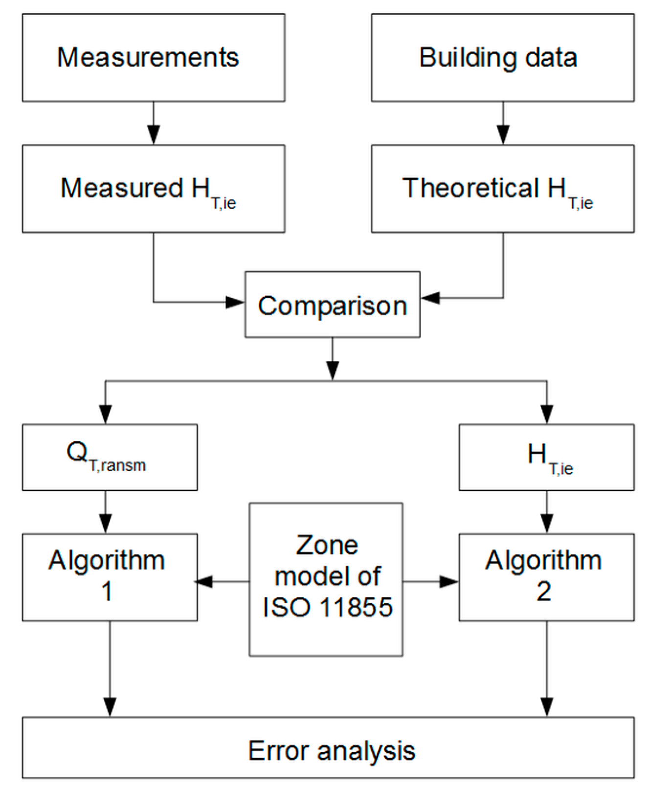
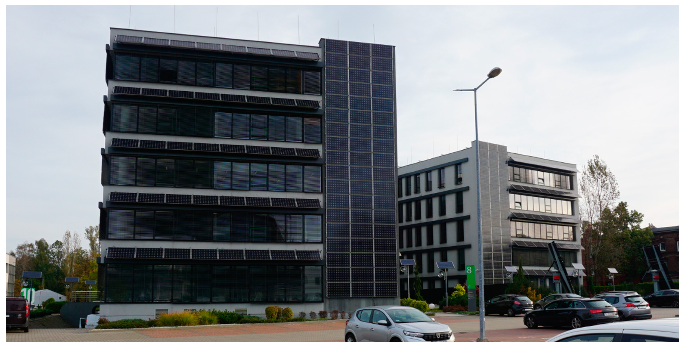
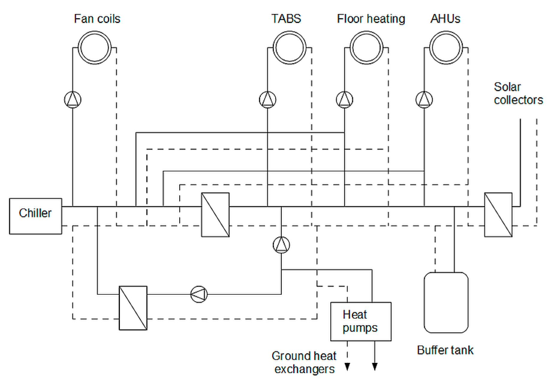
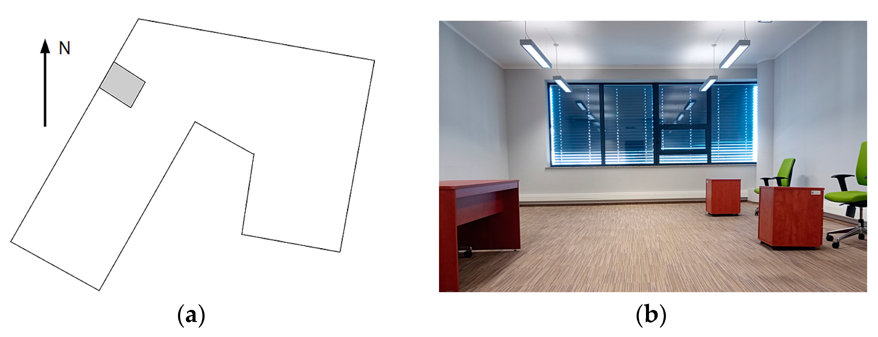
2.1. Research Object and Research Algorithm
2.2. Measurements
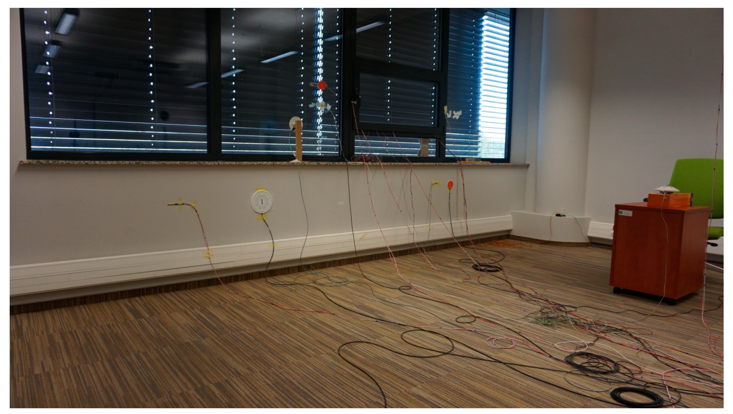
2.2.1. Measurement Campaign
2.2.2. Uncertainty Analysis
2.3. Simulation Model
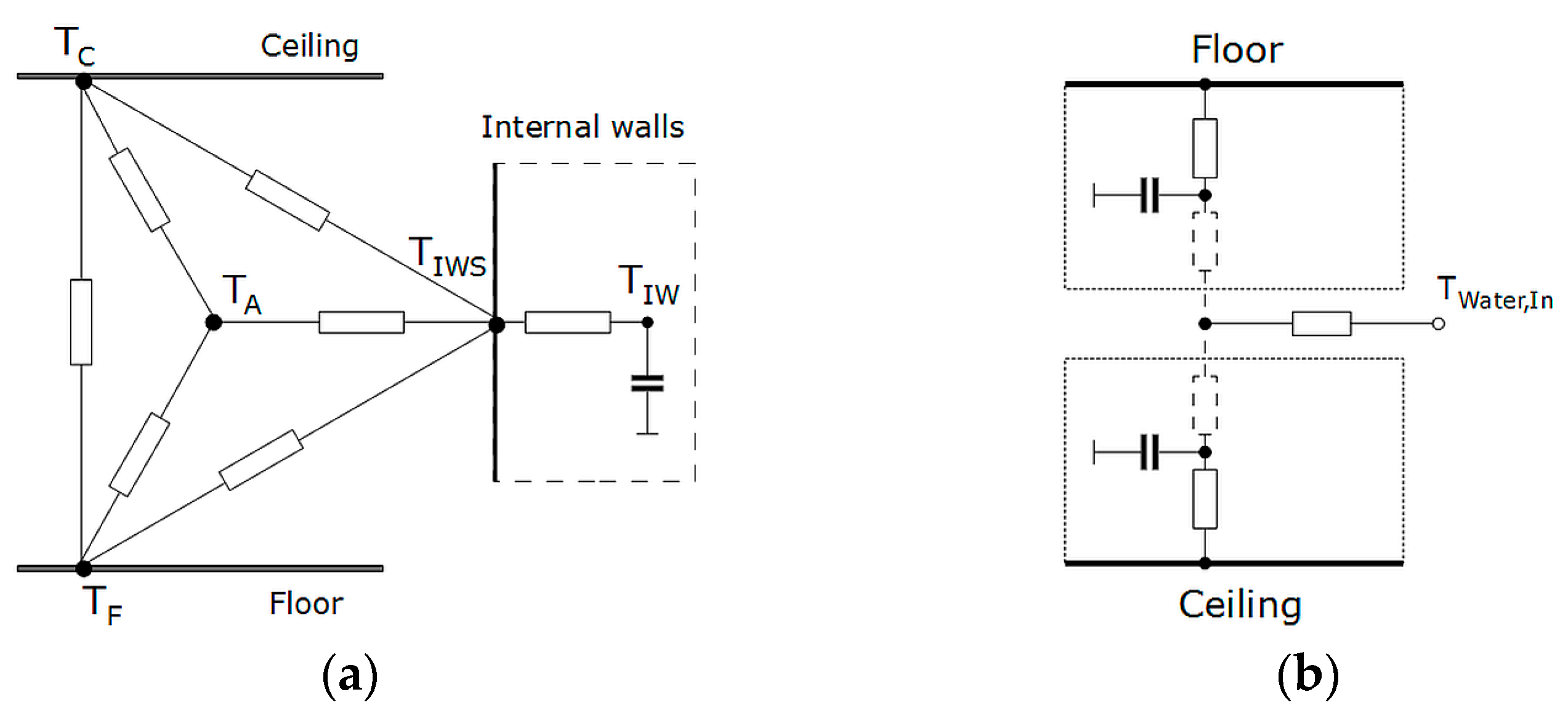
2.3.1. General Description of the Model
- The slab must be without gaps (e.g., suspended ceiling, free spaces under the floor);
- Three-dimensional heat transfer phenomena in a slab were simplified to one-dimensional. Consequently, homogeneous temperature distribution in a slab in the horizontal direction was assumed;
- Radiant heat gains are evenly distributed on all internal surfaces;
- Thermal conditions in adjacent zones are the same as in the studied one;
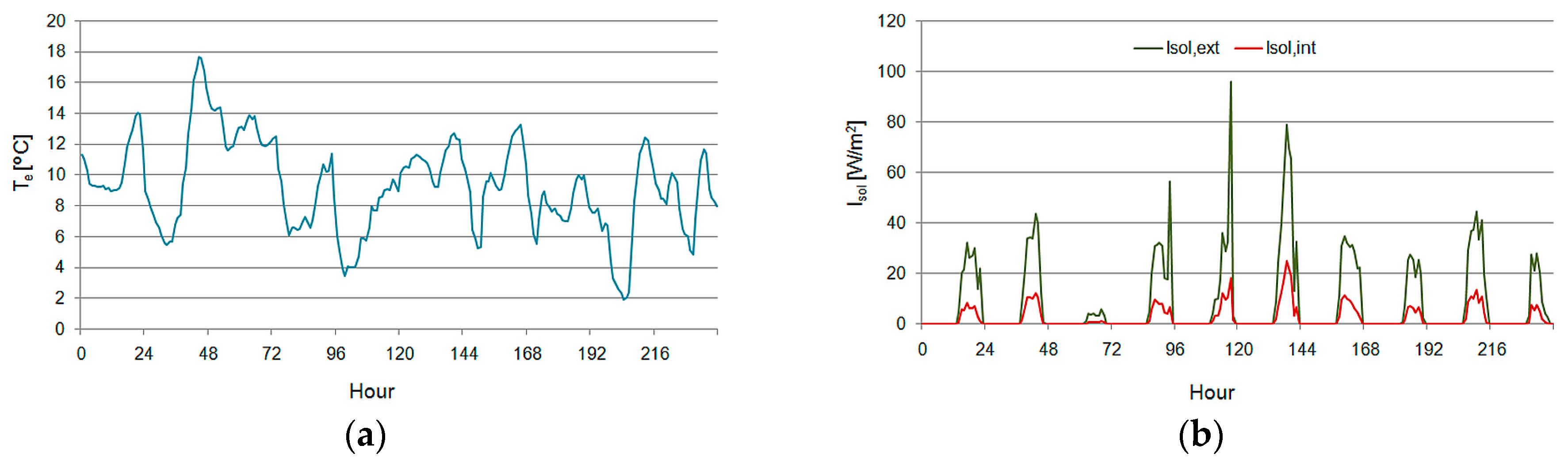
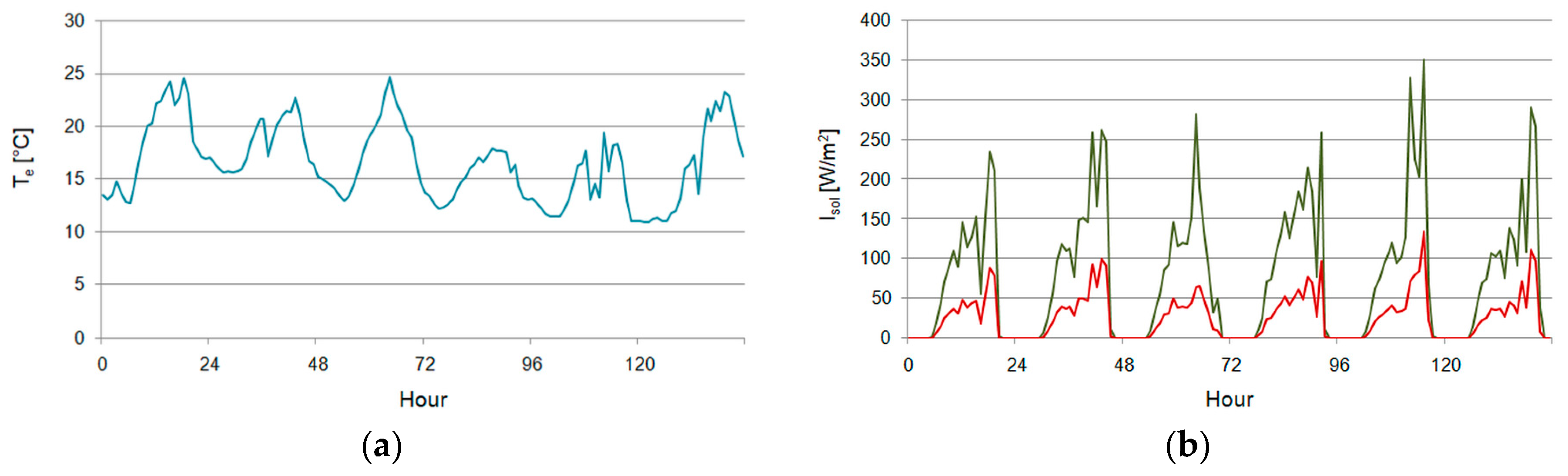
2.3.2. Input Conditions
2.3.3. Heat Transfer by Transmission

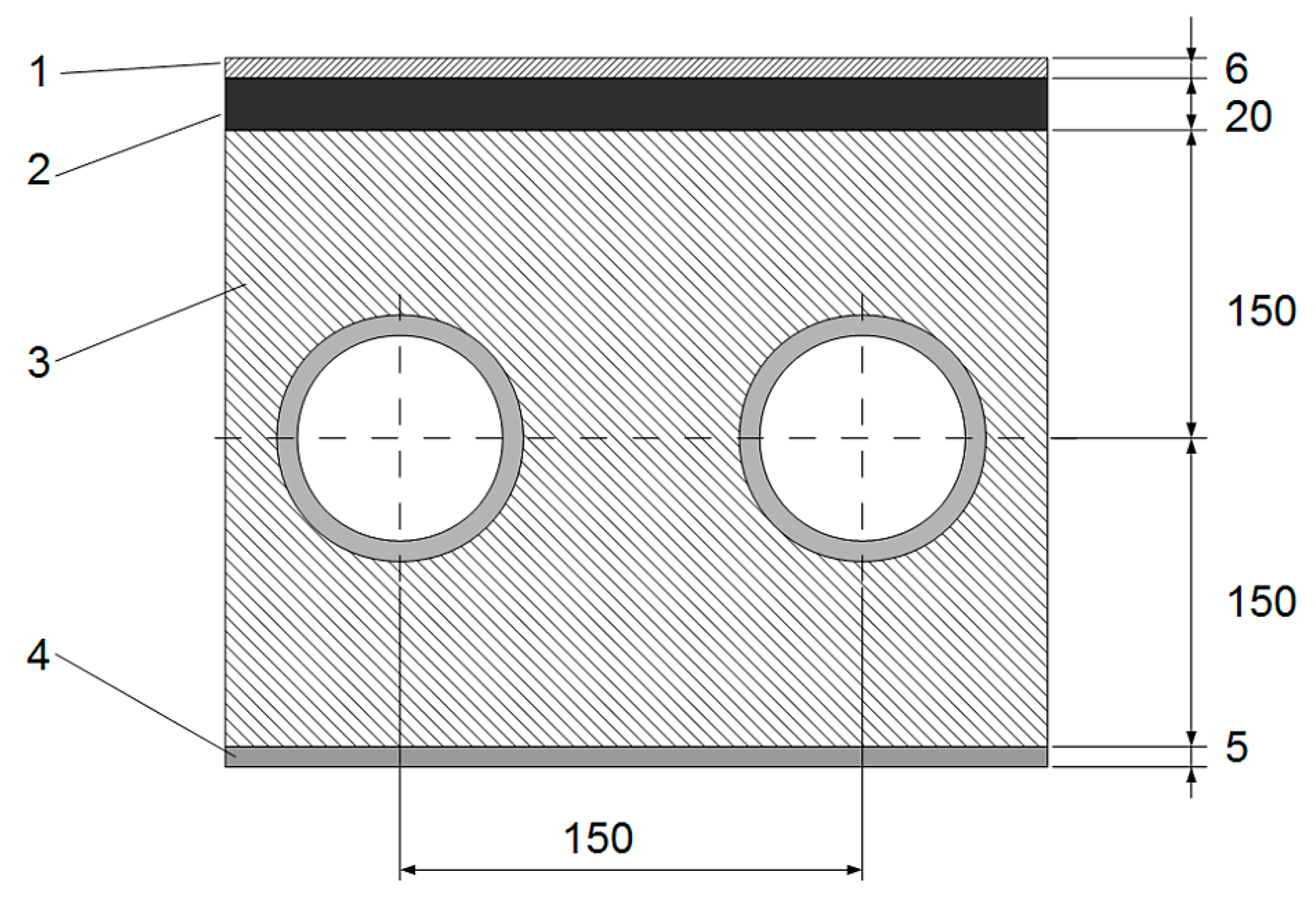
| Partition | Material | Thickness (mm) | Thermal Conductivity W/(m·K) |
|---|---|---|---|
| Floor | Floor covering | 6 | 0.1875 |
| Cement screed | 20 | 1.4 | |
| Reinforced concrete | 300 | 1.9 | |
| Gypsum plastering | 5 | 1.18 | |
| Internal wall | Gypsum board | 25 | 0.24 |
| Mineral wool | 70 | 0.04 | |
| Gypsum board | 25 | 0.24 | |
| External wall | External plaster | 5 | 0.70 |
| Styrofoam | 300 | 0.031 | |
| Ceramic blocks | 300 | 0.23 | |
| Internal plaster | 15 | 0.18 |
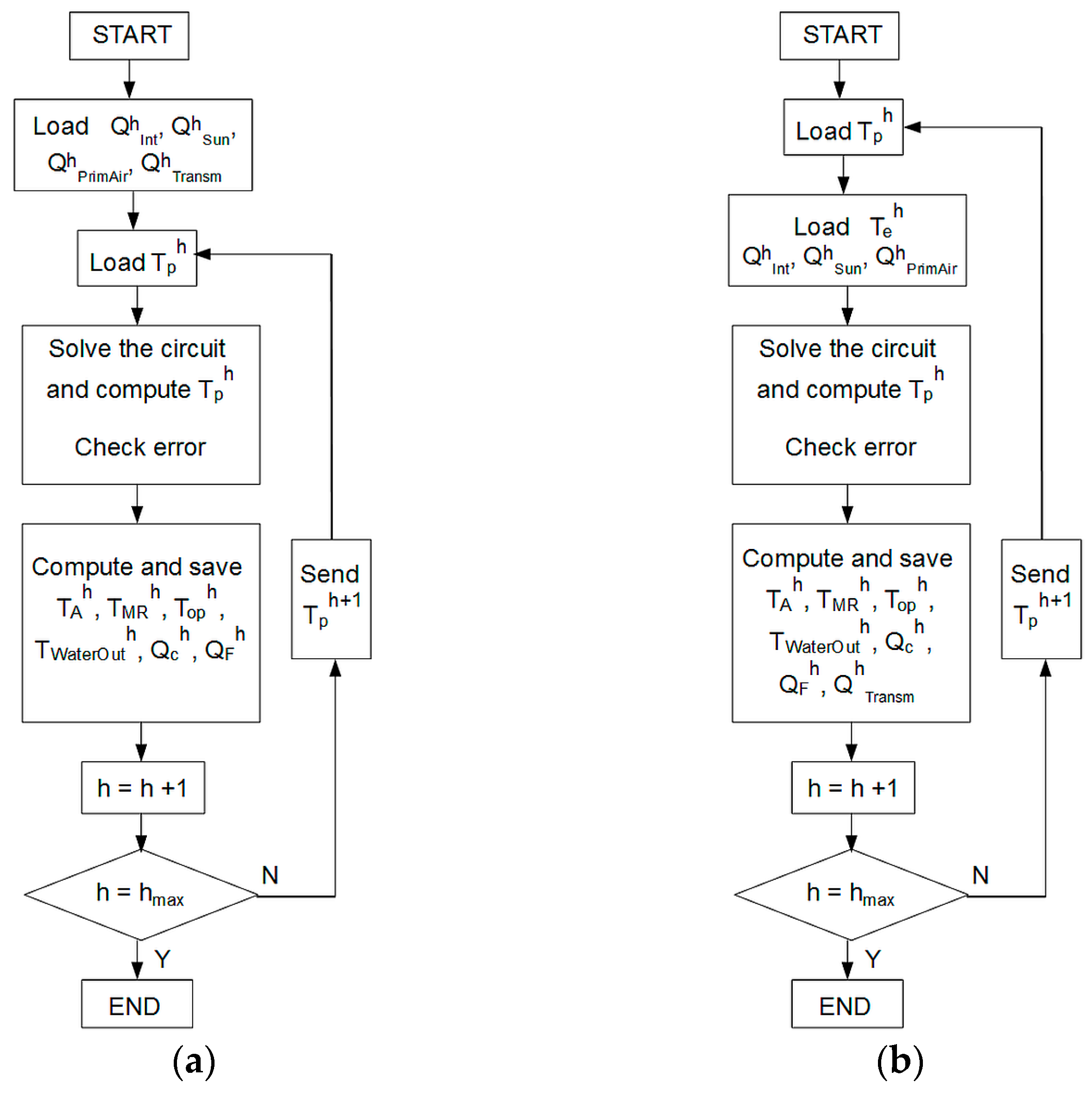
2.3.4. Calculation Algorithm
2.4. Statistical Analysis
3. Results and Discussion
3.1. Thermal Transmittance of the Wall
3.1.1. Results of Measurements
3.1.2. Measurement Uncertainties
3.2. Thermal Transmittance of the Window
3.3. Total Heat Transfer by Transmission
- using measured thermal resistances of the wall and glazing;
- using declared, theoretical values of the materials parameters.
3.4. Simulations
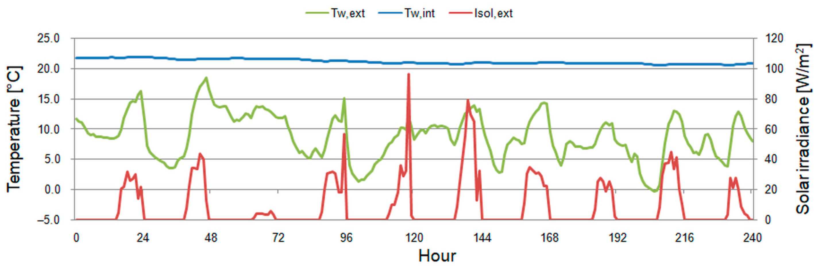
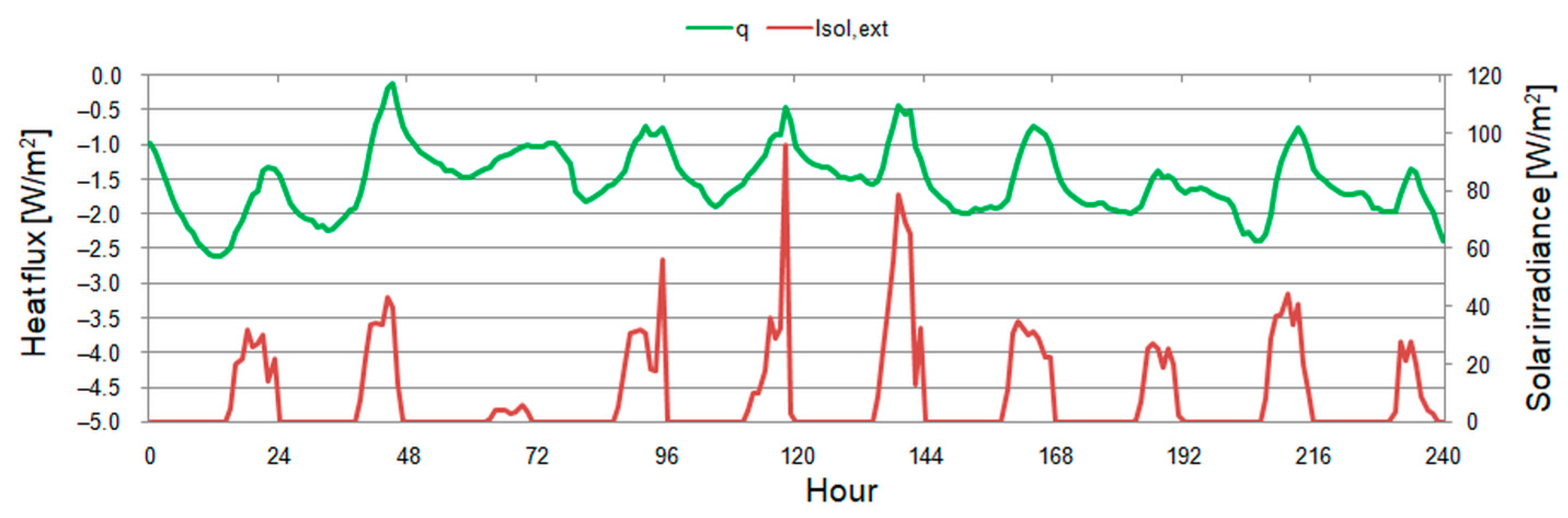
3.4.1. First Period
3.4.2. Second Period
4. Conclusions
Funding
Data Availability Statement
Acknowledgments
Conflicts of Interest
Symbols and Abbreviations
| H | Heat transfer coefficient |
| Isol | Solar irradiance |
| Q | Heat gain |
| R | Thermal resistance |
| T | Temperature |
| u | Uncertainty |
| U | Thermal transmittance |
| Subscripts | |
| A | Air |
| C | Ceiling |
| CondDown | Conduction to next node |
| CondUp | Conduction to previous node |
| Conv | Convective |
| dev | Device |
| EW | External wall (opaque) |
| e | External |
| F | Floor |
| g | Glazing |
| h | Time step number |
| Int | Internal |
| IntConv | Internal convective |
| IntRad | Internal radiant |
| IWS | Internal wall surface |
| MR | Mean radiant |
| p | Node number |
| Rad | Radiant |
| sens | Sensor |
| tot | Total |
| Transm | Transmission |
| W | Window |
| WaterIn | Water inlet |
| Abbreviations | |
| BMS | Building management system |
| FDM | Finite difference method |
| HVAC | Heating, ventilation, and air conditioning |
| MAE | mean absolute error |
| MAPE | mean absolute of percentage error |
| MSE | mean square error |
| RMSE | root mean square error |
| TABS | Thermally activated building systems |
References
- Hawks, M.A.; Cho, S. Review and Analysis of Current Solutions and Trends for Zero Energy Building (ZEB) Thermal Systems. Renew. Sustain. Energy Rev. 2024, 189, 114028. [Google Scholar] [CrossRef]
- Krajčík, M.; Šimko, M.; Šikula, O.; Szabó, D.; Petráš, D. Thermal performance of a radiant wall heating and cooling system with pipes attached to thermally insulating bricks. Energy Build. 2021, 246, 111122. [Google Scholar] [CrossRef]
- Junasová, B.; Krajčík, M.; Šikula, O.; Arıcı, M.; Šimko, M. Adapting the construction of radiant heating and cooling systems for building retrofit. Energy Build. 2022, 268, 112228. [Google Scholar] [CrossRef]
- ISO 11855-2:2021; Building Environment Design. Embedded Radiant Heating and Cooling Systems. Part 2: Determination of the Design Heating and Cooling Capacity. International Organization for Standardization: Geneva, Switzerland, 2021.
- Olesen, B.W. Radiant heating and cooling by embedded water-based systems. In Proceedings of the Congreso Climaplus 2011-I Congreso de Climatización Eficiente, Milan, Italy; 2011. Available online: https://orbit.dtu.dk/en/publications/radiant-heating-and-cooling-by-embedded-water-based-systems (accessed on 12 February 2025).
- ISO 11855-4:2021; Building Environment Design—Desig Installation and Control of Embedded Cooling Systems: Part 4: Dimensioning and Calculation of the Dynamic Heating and Cooling Capacity of Thermo Active Building Systems (TABS). International Organization for Standardization: Geneva, Switzerland, 2021.
- Michalak, P. Selected Aspects of Indoor Climate in a Passive Office Building with a Thermally Activated Building System: A Case Study from Poland. Energies 2021, 14, 860. [Google Scholar] [CrossRef]
- Behrendt, B. Possibilities and Limitations of Thermally Activated Building Systems. Simply TABS and a Climate Classification for TABS. Ph.D. Thesis, Technical University of Denmark, Kongens Lyngby, Denmark, 2016. [Google Scholar]
- Ning, B.; Chen, Y.; Jia, H. A response factor method to quantify the dynamic performance for pipe-embedded radiant systems. Energy Build. 2021, 250, 111311. [Google Scholar] [CrossRef]
- Domínguez Lacarte, L.M.; Fan, J. Modelling of a thermally activated building system (TABS) combined with free-hanging acoustic ceiling units using computational fluid dynamics (CFD). Build. Simul. 2018, 11, 315–324. [Google Scholar] [CrossRef]
- Henze, G.P.; Felsmann, C.; Kalz, D.E.; Herkel, S. Primary energy and comfort performance of ventilation assisted thermo-active building systems in continental climates. Energy Build. 2008, 40, 99–111. [Google Scholar] [CrossRef]
- Nageler, P.; Schweiger, G.; Pichler, M.; Brandl, D.; Mach, T.; Heimrath, R.; Schranzhofer, H.; Hochenauer, C. Validation of dynamic building energy simulation tools based on a real test-box with thermally activated building systems (TABS). Energy Build. 2018, 168, 42–55. [Google Scholar] [CrossRef]
- Chandrashekar, R.; Kumar, B. Experimental investigation on energy saving potential for thermally activated buildings integrated with the active cooling system. Energy Sources Part A Recovery Util. Environ. Eff. 2022, 44, 7585–7597. [Google Scholar] [CrossRef]
- Li, Y.; Mc Lauchlan, C.; Gong, X.; Ma, Z. Experimental and modeling investigation of thermally activated building systems integrated with ground source heat pump systems. Energy Build. 2025, 328, 115210. [Google Scholar] [CrossRef]
- Chen, Q.; Li, N. Model Predictive Control for Energy-efficient Optimization of Radiant Ceiling Cooling Systems. Build. Environ. 2021, 205, 108272. [Google Scholar] [CrossRef]
- Hu, M.; Xiao, F.; Jorgensen, J.B.; Li, R. Price-responsive model predictive control of floor heating systems for demand response using building thermal mass. Appl. Therm. Eng. 2019, 153, 316–329. [Google Scholar] [CrossRef]
- Vivek, T.; Balaji, K. Heat transfer and thermal comfort analysis of thermally activated building system in warm and humid climate—A case study in an educational building. Int. J. Therm. Sci. 2023, 183, 107883. [Google Scholar] [CrossRef]
- Chandrashekar, R.; Kumar, B. Experimental investigation of thermally activated building system under the two different floor covering materials to maximize the underfloor cooling efficiency. Int. J. Therm. Sci. 2023, 188, 108223. [Google Scholar] [CrossRef]
- Zhen, J.; Lu, J.; Huang, G.; Zhang, H. Groundwater source heat pump application in the heating system of Tibet Plateau airport. Energy Build. 2017, 136, 33–42. [Google Scholar] [CrossRef]
- Mugnini, A.; Evens, M.; Arteconi, A. Model predictive controls for residential buildings with heat pumps: Experimentally validated archetypes to simplify the large-scale application. Energy Build. 2024, 320, 114632. [Google Scholar] [CrossRef]
- Ye, M.; Serageldin, A.A.; Radwan, A.M.; Hideki, S.; Katsunori, N. Thermal performance of ceiling radiant cooling panel with a segmented and concave surface. Laboratory analysis. Appl. Therm. Eng. 2021, 196, 117280. [Google Scholar] [CrossRef]
- Sinacka, J.; Mróz, T. Novel radiant heating and cooling panel with a monolithic aluminium structure and U-groove surface—Experimental investigation and numerical model. Appl. Therm. Eng. 2023, 229, 120611. [Google Scholar] [CrossRef]
- Pawlak, F.; Koczyk, H.; Górka, A. 3D numerical model for transient simulations of floor cooling capacity and thermal comfort in a thermally heterogeneous room. Build. Environ. 2023, 245, 110903. [Google Scholar] [CrossRef]
- Werner-Juszczuk, A.J. Analysis of the Use of Radiant Floor Heating as a Cooling System. Proceedings 2019, 16, 23. [Google Scholar] [CrossRef]
- Langiu, M.; Shu, D.Y.; Baader, F.J.; Hering, D.; Bau, U.; Xhonneux, A.; Müller, D.; Bardow, A.; Mitsos, A.; Dahmen, M. COMANDO: A Next-Generation Open-Source Framework for Energy Systems Optimization. Comput. Chem. Eng. 2021, 152, 107366. [Google Scholar] [CrossRef]
- Putz, D.; Gumhalter, M.; Auer, H. The true value of a forecast: Assessing the impact of accuracy on local energy communities. Sustain. EnergyGrids Netw. 2023, 33, 100983. [Google Scholar] [CrossRef]
- Sharifi, M.; Mahmoud, R.; Himpe, E.; Laverge, J. A heuristic algorithm for optimal load splitting in hybrid thermally activated building systems. J. Build. Eng. 2022, 50, 104160. [Google Scholar] [CrossRef]
- Szpytma, M.; Rybka, A. Ecological ideas in Polish architecture—Environmental impact. J. Civ. Eng. Environ. Arch. 2016, XXXIII, 321–328. [Google Scholar] [CrossRef]
- IEC 60751:2022; Industrial Platinum Resistance Thermometers and Platinum Temperature Sensors. International Electrotechnical Commission: Geneva, Switzerland, 2022.
- ISO 9060:2018; Solar Energy—Specification and Classification of Instruments for Measuring Hemispherical Solar and Direct Solar Radiation. International Organization for Standardization: Geneva, Switzerland, 2018.
- IEC 61724-1:2021; Photovoltaic System Performance-Part 1: Monitoring. International Organization for Standardization: Geneva, Switzerland, 2022.
- HFP03 Heat Flux Sensor. Hukseflux. Available online: https://www.hukseflux.com/products/heat-flux-sensors/heat-flux-sensors/hfp03-heat-flux-sensor (accessed on 12 February 2025).
- HFP01 Heat Flux Sensor. Hukseflux. Available online: https://www.hukseflux.com/products/heat-flux-sensors/heat-flux-sensors/hfp01-heat-flux-sensor (accessed on 12 February 2025).
- Asdrubali, F.; D’Alessandro, F.; Baldinelli, G.; Bianchi, B. Evaluating in situ thermal transmittance of green buildings masonries—A case study. Case Stud. Constr. Mater. 2014, 1, 53–59. [Google Scholar] [CrossRef]
- Ohlsson, K.E.A.; Östin, R.; Olofsson, T. Accurate and robust measurement of the external convective heat transfer coefficient based on error analysis. Energy Build. 2016, 117, 83–90. [Google Scholar] [CrossRef]
- Chen, J.; Chen, C. Uncertainty Analysis in Humidity Measurements by the Psychrometer Method. Sensors 2017, 17, 368. [Google Scholar] [CrossRef]
- Chen, L.-H.; Chen, J.; Chen, C. Effect of Environmental Measurement Uncertainty on Prediction of Evapotranspiration. Atmosphere 2018, 9, 400. [Google Scholar] [CrossRef]
- Madejski, P.; Michalak, P.; Karch, M.; Kuś, T.; Banasiak, K. Monitoring of Thermal and Flow Processes in the Two-Phase Spray-Ejector Condenser for Thermal Power Plant Applications. Energies 2022, 15, 7151. [Google Scholar] [CrossRef]
- PN EN 12831-1: 2017; Energy Performance of Buildings—Method for Calculation of the Design Heat Load. Polish Committee of Standardisation: Warsaw, Poland, 2017.
- ISO10077-1:2017; Thermal Performance of Windows, Doors and Shutters—Calculation of Thermal Transmittance. ISO: Geneva, Switzerland, 2017.
- EN ISO 6946; Building Components and Building Elements—Thermal Resistance and Thermal Transmittance–Calculation Methods. ISO: Geneva, Switzerland, 2007.
- Deconinck, A.H.; Roels, S. Comparison of Characterisation Methods Determining the Thermal Resistance of Building Components from Onsite Measurements. Energy Build. 2016, 130, 309–320. [Google Scholar] [CrossRef]
- Anderlind, G. Multiple Regression Analysis of Thermal Measurements–Study of an Attic Insulated with 800 mm Loose. J. Build. Phys. 1992, 61, 81–104. [Google Scholar] [CrossRef]
- Anderlind, G.; Dynamic Thermal Models. Dynamic Thermal Models. Two dynamic Models for Estimating Thermal Resistance and Heat Capacity from in situ measurements. Swedish Council for Building Research, BFR. 1996. Available online: https://www.academia.edu/33093591/BFR_Dynamic_Thermal_Models (accessed on 12 February 2025).
- Lu, X.; Memari, A.M. Comparison of the Experimental Measurement Methods for Building Envelope Thermal Transmittance. Buildings 2022, 12, 282. [Google Scholar] [CrossRef]
- Lorenz, F.; Masy, G. Méthoded’évaluation de l’économied’énergieapportée par l’intermittence de chauffage dans les bâtiments. In Traitement par Differences Finies d’un Model a deux Constantes de Temps; Report No. GM820130-01; Faculte des Sciences Appliquees, University de Liege: Liege, Belgium, 1982. [Google Scholar]
- Dimitriou, V.; Firth, S.K.; Hassan, T.M.; Kane, T. The applicability of Lumped Parameter modelling in houses using in-situ measurements. Energy Build. 2020, 223, 110068. [Google Scholar] [CrossRef]
- Adeala, A.A.; Huan, Z.; Enweremadu, C.C. Evaluation of global solar radiation using multiple weather parameters as predictors for South Africa Provinces. Therm. Sci. 2015, 19, 495–509. [Google Scholar] [CrossRef]
- Pham, H. A New Criterion for Model Selection. Mathematics 2019, 7, 1215. [Google Scholar] [CrossRef]
- Wang, X.; Liu, X.; Wang, Y.; Kang, X.; Geng, R.; Li, A.; Xiao, F.; Zhang, C.; Yan, D. Investigating the deviation between prediction accuracy metrics and control performance metrics in the context of an ice-based thermal energy storage system. J. Energy Storage 2024, 91, 112126. [Google Scholar] [CrossRef]
- ISO 10456:2007; Building Materials and Products—Hygrothermal Properties—Tabulated Design Values and Procedures for Determining Declared and Design Thermal Values. ISO: Geneva, Switzerland, 2007.
- ISO 7730; Ergonomics of the Thermal Environment—Analytical Determination and Interpretation of Thermal Comfort Using Calculation of the PMV and PPD Indices and Local Thermal Comfort Criteria. International Organisation for Standardization: Geneva, Switzerland, 2005.
- EN 1264-2; Water Based Surface Embedded Heating and Cooling Systems-Part 2: Floor Heating: Prove Methods for the Determination of the Thermal Output Using Calculation and Test Methods. European Committee for Standardization: Brussels, Belgium, 2012.
- Werner-Juszczuk, A.J. The influence of the thickness of an aluminium radiant sheet on the performance of the lightweight floor heating. J. Build. Eng. 2021, 44, 102896. [Google Scholar] [CrossRef]
- Ohlsson, K.E.A.; Olofsson, T. Benchmarking the practice of validation and uncertainty analysis of building energy models. Renew. Sustain. Energy Rev. 2021, 142, 110842. [Google Scholar] [CrossRef]

| Device | Measured Variable | Measurement Range | Accuracy |
|---|---|---|---|
| Pt100 resistance sensor | Indoor air temperature | −50 °C … +150 °C | Class AA 1 |
| Pt100 resistance sensor | Surface temperature | −50 °C … +150 °C | Class AA 1 |
| Pt1000 resistance sensor | Ambient air temperature | −50 °C … +150 °C | Class A 1 |
| Pt100 resistance sensor | Globe temperature | −30 °C … +120 °C | Class A 1 |
| LP PYRA03 | Solar irradiance | 0 … 2000 W/m2 | Spectrally Flat Class C 2 |
| HFP01 Hukseflux | Window heat flux | −2000 … 2000 W/m2 | ±3% 3 |
| HFP03 Hukseflux | Wall heat flux | −2000 … 2000 W/m2 | ±6% 3 |
| Fluke 2638A data logger | Voltage input | 0 … 100 mV | 0.0025% MV + 0.0035% FS + 2 μV 4 |
| Fluke 2638A data logger | Temperature input | −50 °C … +150 °C | 0.038 °C at 0 °C, 0.073 °C at 300 °C |
| Uncertainty | Value | Unit |
|---|---|---|
| u(Twi) | 0.093 | K |
| u(Twe) | 0.082 | K |
| u(q) | 0.135 | W/m2 |
| –0.595 | W/m2K | |
| 0.595 | W/m2K | |
| –4.915 | W/m2K2 |
| Parameter | Measured (Static) | Measured (Dynamic) | Theoretical | Unit |
|---|---|---|---|---|
| HT,ie | 10.51 | 10.37 | 10.33 | W/K |
| Error | Variant 1 | Variant 2 | Variant 3 | Variant 4 | Unit |
|---|---|---|---|---|---|
| MAE | 0.13 | 0.13 | 0.14 | 0.24 | °C |
| RMSE | 0.17 | 0.16 | 0.17 | 0.28 | °C |
| MSE | 0.03 | 0.03 | 0.03 | 0.08 | °C2 |
| MAPE | 0.65 | 0.61 | 0.65 | 1.15 | % |
| Error | Variant 1 | Variant 2 | Variant 3 | Variant 4 | Unit |
|---|---|---|---|---|---|
| MAE | 0.12 | 0.12 | 0.12 | 0.21 | °C |
| RMSE | 0.14 | 0.15 | 0.15 | 0.24 | °C |
| MSE | 0.02 | 0.02 | 0.02 | 0.06 | °C2 |
| MAPE | 0.54 | 0.55 | 0.57 | 0.98 | % |
| Error | Variant 1 | Variant 2 | Variant 3 | Variant 4 | Unit |
|---|---|---|---|---|---|
| MAE | 0.18 | 0.19 | 0.19 | 0.12 | °C |
| RMSE | 0.22 | 0.23 | 0.23 | 0.15 | °C |
| MSE | 0.05 | 0.05 | 0.05 | 0.02 | °C2 |
| MAPE | 0.81 | 0.87 | 0.85 | 0.57 | % |
| Error | Variant 1 | Variant 2 | Variant 3 | Variant 4 | Unit |
|---|---|---|---|---|---|
| MAE | 0.15 | 0.16 | 0.16 | 0.14 | °C |
| RMSE | 0.19 | 0.20 | 0.20 | 0.17 | °C |
| MSE | 0.04 | 0.04 | 0.04 | 0.03 | °C2 |
| MAPE | 0.69 | 0.73 | 0.75 | 0.65 | % |
| Error | Variant 1 | Variant 2 | Variant 3 | Variant 4 | Unit |
|---|---|---|---|---|---|
| MAE | 0.17 | 0.14 | 0.14 | 0.14 | °C |
| RMSE | 0.20 | 0.20 | 0.18 | 0.20 | °C |
| MSE | 0.04 | 0.04 | 0.03 | 0.04 | °C2 |
| MAPE | 0.76 | 0.64 | 0.62 | 0.64 | % |
| Error | Variant 1 | Variant 2 | Variant 3 | Variant 4 | Unit |
|---|---|---|---|---|---|
| MAE | 0.15 | 0.16 | 0.15 | 0.16 | °C |
| RMSE | 0.26 | 0.26 | 0.26 | 0.26 | °C |
| MSE | 0.07 | 0.07 | 0.07 | 0.07 | °C2 |
| MAPE | 0.69 | 0.69 | 0.69 | 0.69 | % |
| Error | Variant 1 | Variant 2 | Variant 3 | Variant 4 | Unit |
|---|---|---|---|---|---|
| MAE | 0.19 | 0.15 | 0.18 | 0.15 | °C |
| RMSE | 0.23 | 0.18 | 0.21 | 0.18 | °C |
| MSE | 0.05 | 0.03 | 0.05 | 0.03 | °C2 |
| MAPE | 0.90 | 0.68 | 0.82 | 0.69 | % |
| Error | Variant 1 | Variant 2 | Variant 3 | Variant 4 | Unit |
|---|---|---|---|---|---|
| MAE | 0.11 | 0.10 | 0.08 | 0.10 | °C |
| RMSE | 0.13 | 0.13 | 0.10 | 0.13 | °C |
| MSE | 0.02 | 0.02 | 0.01 | 0.01 | °C2 |
| MAPE | 0.50 | 0.46 | 0.38 | 0.46 | % |
Disclaimer/Publisher’s Note: The statements, opinions and data contained in all publications are solely those of the individual author(s) and contributor(s) and not of MDPI and/or the editor(s). MDPI and/or the editor(s) disclaim responsibility for any injury to people or property resulting from any ideas, methods, instructions or products referred to in the content. |
© 2025 by the author. Licensee MDPI, Basel, Switzerland. This article is an open access article distributed under the terms and conditions of the Creative Commons Attribution (CC BY) license (https://creativecommons.org/licenses/by/4.0/).
Share and Cite
Michalak, P. Heat Transfer by Transmission in a Zone with a Thermally Activated Building System: An Extension of the ISO 11855 Hourly Calculation Method. Measurement and Simulation. Energies 2025, 18, 2350. https://doi.org/10.3390/en18092350
Michalak P. Heat Transfer by Transmission in a Zone with a Thermally Activated Building System: An Extension of the ISO 11855 Hourly Calculation Method. Measurement and Simulation. Energies. 2025; 18(9):2350. https://doi.org/10.3390/en18092350
Chicago/Turabian StyleMichalak, Piotr. 2025. "Heat Transfer by Transmission in a Zone with a Thermally Activated Building System: An Extension of the ISO 11855 Hourly Calculation Method. Measurement and Simulation" Energies 18, no. 9: 2350. https://doi.org/10.3390/en18092350
APA StyleMichalak, P. (2025). Heat Transfer by Transmission in a Zone with a Thermally Activated Building System: An Extension of the ISO 11855 Hourly Calculation Method. Measurement and Simulation. Energies, 18(9), 2350. https://doi.org/10.3390/en18092350