Article

Research on Coordinated Control of Dynamic Reactive Power Sources of DC Blocking and Commutation Failure Transient Overvoltage in New Energy Transmission

1
College of Instrumentation and Electrical Engineering, Jilin University, Changchun 130061, China
2
China Electric Power Research Institute, Beijing 100192, China
*
Author to whom correspondence should be addressed.
Energies 2025, 18(9), 2349; https://doi.org/10.3390/en18092349
Submission received: 30 March 2025 / Revised: 28 April 2025 / Accepted: 2 May 2025 / Published: 4 May 2025

Abstract

:
With the large-scale deployment of renewable energy, transmission systems for new energy sources are increasingly exposed to transient overvoltage issues induced by DC blockages and commutation failures. To address the challenges of an imprecise response to multiple fault scenarios and the inefficiency of independent device actions in existing dynamic reactive power control schemes, this paper proposes a coordinated optimization control strategy integrating multiple dynamic reactive power sources tailored to different fault characteristics. An equivalent model of the renewable energy DC transmission system is established to elucidate the underlying mechanisms of transient overvoltage formation under various fault conditions. By employing trajectory sensitivity analysis and parameter perturbation methods, the influence patterns of control parameters on transient overvoltage behaviors across different fault scenarios are quantitatively assessed, thereby overcoming the limitations of traditional empirical parameter tuning approaches. Subsequently, a multi-source coordinated optimization model is developed with the objective of minimizing transient overvoltages under simultaneous dual-fault conditions. A multi-objective particle swarm optimization algorithm, incorporating comprehensive trajectory sensitivity and dynamically adaptive inertia weights, is introduced, alongside Pareto front theory, to achieve rapid and balanced optimization among competing objectives. Simulation results validate that the proposed strategy significantly enhances transient overvoltage suppression across diverse fault conditions. The findings provide robust theoretical foundations and practical guidance for the refined parameter tuning and high-efficiency coordinated control of dynamic reactive power sources in renewable energy transmission systems.

1. Introduction

Driven by the global energy transition and the “dual carbon” goals, the rapid development of new energy, represented by wind and photovoltaic (PV) power, is taking place [1]. High-voltage direct current (HVDC) transmission technology, with its advantages in long-distance, large-capacity, and low-loss transmission, has become the core carrier for new energy delivery [2]. Under the context of large-scale new energy delivery, the security and stable operation of the system faces significant challenges. Transient overvoltage, as a typical fault phenomenon, has become a key bottleneck restricting new energy delivery capacity and system security. Therefore, in current engineering practices, dynamic reactive power source equipment is mainly relied upon to suppress transient overvoltage [3].
In the field of new energy control, Adireddy et al. compared the overvoltage suppression effects of different transformer configurations and grounding techniques from the perspective of photovoltaic systems, providing technical references for transient voltage control in distributed new energy grid integration [4]. Mohseni et al. studied the transient process and improved control strategies in doubly fed induction generators (DFIGs) when the voltage suddenly increases, using hysteresis controllers to replace PI controllers or introducing resonant controllers as supplements to enhance the system’s dynamic response speed [5]. Amin et al. proposed a strategy to replace traditional PI control with hysteresis controllers to improve the transient overvoltage response speed of wind turbines, but the control algorithm still faces difficulties and it is challenging to suppress transient overvoltage by optimizing the wind turbine’s own control strategy [6].
In the field of DC control, Liang et al. addressed the overvoltage issue caused by commutation failure at the sending end of LCC-HVDC rectifier stations, proposing methods to enhance the rectifier’s reactive power absorption and increase the inverter-side extinction angle to suppress transient overvoltage caused by excessive reactive power from the filter [7]. Yin et al. proposed a constant reactive power control (CRPC) strategy, which effectively suppresses transient overvoltage by enhancing the rectifier’s reactive power absorption and reducing the reactive power exchange between AC and DC systems [8]. Wang et al. proposed a DC current reference limit method based on AC overvoltage sampling, which accelerates the DC current recovery to suppress overvoltage and prevent the disconnection of new energy units from the grid in an unordered manner [9]. Mannen et al. proposed a multi-instantaneous short-circuit strategy based on the power devices of converter bridge arms, aiming to release resonant energy to suppress overvoltage and achieve coordinated optimization between overvoltage mitigation and system compactness [10]. Maruta et al. investigated a neural network control strategy for digitally controlled PWM converters, proposing a suppression method that estimates the current based on the steady-state output voltage equation [11]. By dynamically switching control modes, the approach enhances transient response while eliminating overcompensation caused by system delays and computational nonlinearities.
In the field of dynamic reactive power sources, Hamdan et al. proposed the use of STATCOM in wind–solar hybrid systems to enhance fault ride-through capability by dynamically adjusting the reactive power at the point of common coupling (PCC) to suppress voltage sags. Compared to the traditional reactive power injection combined with crowbar FRT strategy, this method can maintain PV active output and reduce wind turbine speed oscillations, avoiding DC link overvoltage [12]. Guo et al. addressed the issue of grid-connected offshore PV frequency overvoltage (IFOV), revealing the mechanism of IFOV caused by cable capacitance effects and proposing a reactive power compensation solution based on SVG which dynamically adjusts capacitive reactive power to suppress overvoltage and optimize system compensation capability [13]. Wu et al. pointed out that the main cause of transient overvoltage in new energy bases is transient reactive power surplus and proposed a dynamic multi-reactive power source configuration scheme, combining synchronous compensators and STATCOMs: the compensators provide instantaneous reactive power support and the STATCOMs dynamically compensate to accelerate voltage recovery and suppress overvoltage peaks [14]. Manuela et al. revealed that the primary cause of low-voltage ride-through (LVRT) voltage instability in fixed-speed induction generator wind farms is reactive power overload caused by large rotor slip, and the dynamic models of STATCOM/SVC confirmed the critical impact of their capacity configuration on transient voltage recovery [15]. Pathak et al. quantified the differential impact of SVC placement on static/dynamic reactive power suppression in wind power systems, revealing the optimization mapping relationship between spatial configuration and voltage stability [16].
In summary, existing research focuses mainly on the control of wind turbines, PV systems, and DC lines. Reactive power source control adjustments often rely on empirical or model-based tuning, lacking systematic analysis of control parameters, and it is difficult to achieve fine-tuned control in different fault scenarios. Most research focuses on independent reactive power compensation for transient voltage at individual device access points, failing to fully consider the complementary and conflicting dynamic responses of multiple dynamic reactive power sources, and does not adequately balance the suppression requirements of DC blocking and commutation failure scenarios.
This paper primarily addresses the above issues. Firstly, it analyzes the causes of transient overvoltage after DC blocking and commutation failure faults. Secondly, it quantifies the impact rules of dynamic reactive power source control parameters on transient overvoltage, overcoming the limitations of existing methods where parameter adjustments cannot precisely match the needs of different fault scenarios. Finally, it proposes a collaborative control strategy for multiple dynamic reactive power sources, breaking through the bottleneck of independent control for single devices or simple coordination strategies and achieving efficient suppression of transient overvoltage under the premise of balancing the needs of DC blocking and commutation failure faults.

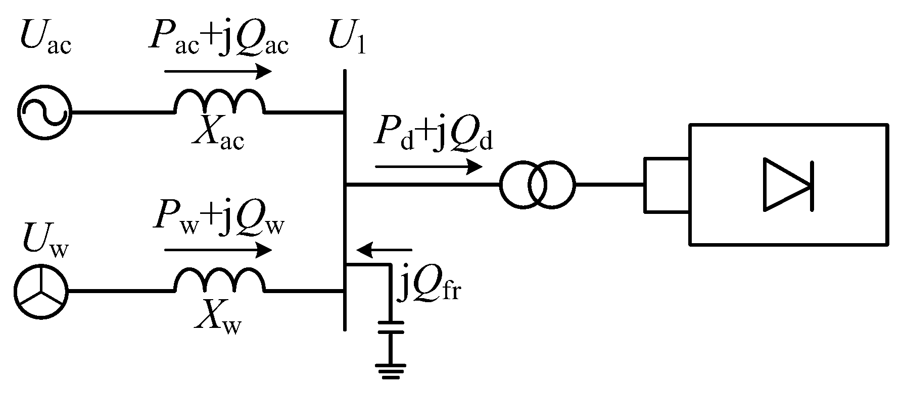
2. Causes of Transient Overvoltage

Currently, the primary method for the large-scale integration of new energy in China is to increase the voltage of each new energy unit through substations, aggregate them, and then transmit the electrical power to DC converter nodes where the energy is then delivered to high-load areas via DC transmission lines. To facilitate the explanation and analysis of the formation mechanism of transient overvoltage, an equivalent system model for wind power transmission via DC is established, as shown in Figure 1.
In a DC transmission system, the rectifier station and inverter station at both ends of the DC line have the following DC bus voltages, respectively:
U d 1 = 3 2 π U 1 cos α 3 π X c 1 I d
U d 2 = 3 2 π U 2 cos β + 3 π X c 2 I d
where U d 1 is the DC bus voltage at the rectifier station; U d 2 is the DC bus voltage at the inverter station; U1 and U2 are the AC bus voltages at the rectifier and inverter stations, respectively; α is the firing angle; β is the lead firing angle; Id is the DC current; and X c 1 and X c 2 are the commutation reactances at the rectifier and inverter stations, respectively.
To facilitate the analysis of the reactive power interaction during transient overvoltage, the equivalent circuit model for the sending end is as shown in Figure 2.
In steady-state operation, the reactive power consumption at the converter station typically accounts for about 40% to 60% of the active power. This reactive power is primarily compensated locally by the filter installed at the AC bus. This portion of reactive power can be expressed as follows:
Q d = U d 1 I d 1 cos φ 1 2   = P d sin 2 α sin 2 ( α + μ ) + 2 μ cos 2 α cos 2 ( α + μ )
where Qd is the reactive power consumed by the sending-end converter station; Pd is the DC power; μ is the commutation overlap angle; and φ 1 is the power factor angle of the sending-end converter station.
From Figure 2, the reactive power balance of the sending end system is as follows:
Q d = Q ac + Q w + Q fr
where Qac is the reactive power output of the sending-end AC system; Qw is the reactive power output of the sending end wind turbine; and Qfr is the reactive power compensation capacity of the sending-end converter station.
After a fault disturbance occurs in the DC transmission line, the reactive power consumed by the sending-end converter station changes. The deviation in the system’s reactive power is as follows:
Δ Q = Q ac + Q w + Q fr Q d
The rise in the AC bus voltage at the sending-end converter station is related to the system’s reactive power surplus and the system’s short-circuit capacity. Its transient voltage rise can be expressed as follows:
Δ U 1 = Δ Q U 1 N U 1 N 2 S c = Δ Q S c U 1 N
where Δ U 1 is the transient voltage rise at the AC bus of the sending-end converter station; Δ Q is the surplus reactive power at the sending-end converter station during a fault; U 1 N is the rated AC bus voltage of the sending-end converter station; and Sc is the short-circuit capacity of the sending end system.
After substituting Equation (5) into Equation (6) and using per-unit values, the transient voltage rise at the AC bus of the sending end can be expressed as follows:
Δ U 1 * = Δ U 1 U 1 N = Δ Q S c = Q ac + Q w + Q fr Q d S c
After the transient voltage rise at the sending end AC bus occurs, its voltage rise will propagate to the wind farm. The propagation Δ U 1 * ( X w ) is inversely correlated with the distance X w between the wind turbine and the sending end AC bus. This voltage propagation to the wind farm results in the transient voltage rise at the wind turbine terminals, which can be expressed as follows:
Δ U w * = [ ( 1 + Δ U 1 * ( X w ) ) 2 1 ] Q w 1 ( + Q wL ) S w
where S w is the short-circuit capacity of the wind farm; Q w 1 is the reactive power generated by the voltage effect after the wind farm receives the voltage Δ U 1 * ( X w ) ; and Q wL is the reactive power during LVRT of the wind turbine under commutation failure, which does not exist under DC blocking conditions.

2.1. DC Blocking

When a DC system experiences blocking, it is equivalent to a circuit breaker occurring in the DC transmission line. The DC bus voltage U d 1 at the sending end rectifier station and the DC line current Id both drop suddenly to zero, causing the DC transmission power Pd to drop to zero. Correspondingly, the reactive power Qd consumed by the converter station, as expressed by Equation (3), also decreases rapidly with the decline in active power. However, due to the addition of local reactive power compensation filters, the AC bus voltage U1 remains relatively high. Due to the delayed response of the actual grid’s security and protection control system, the filter is not promptly disconnected and it continues to emit a large amount of capacitive reactive power Qfr. The surplus reactive power Δ Q , as given by Equation (5), cannot be absorbed in time and accumulates on the AC bus. Ultimately, this leads to overvoltage on the sending end AC bus, as described by Equation (7). After the fault occurs, 100 ms, or 0.3 s later, the compensation filter on the AC side is disconnected and the voltage drops back to normal.
The transient voltage rise Δ U 1 * on the sending end AC bus caused by DC blocking propagates to the wind farm. Due to the fixed capacitive compensators in the wind farm, excessive reactive power Q w 1 is generated by the voltage effect. At this point, the reactive power Q wL generated by the LVRT of the wind turbines does not exist. This results in transient overvoltage at the wind turbine terminals, as described by Equation (8).

2.2. Commutation Failure

When a commutation failure occurs at the inverter side, the previously conducting valve fails to turn off in time, causing both valves in the upper and lower arms to remain simultaneously conducting after the commutation process ends. When both valves conduct simultaneously, a low-impedance loop is formed on the AC side due to a two-phase short circuit. The current that should have flowed through the load is bypassed by the short-circuit path, resulting in an equivalent open circuit on the AC side. Meanwhile, a direct short-circuit path is formed between the positive and negative poles of the DC side, resulting in an equivalent DC side short circuit.
In the initial stage of the fault, the DC line current Id rises sharply, while the sending end DC bus voltage Ud1 remains unaffected. As expressed in Equation (3), the reactive power Qd consumed by the rectifier station increases. Since fixed reactive power compensation devices such as filters cannot immediately supply the required reactive power, the DC transmission system absorbs a large amount of reactive power from the AC network, leading to changes in the reactive power Δ Q , as described in Equation (5). As shown in Equation (7), the change in the sending end AC bus voltage is negative, and the sending end AC bus voltage U1 exhibits a downward trend. Correspondingly, the sending end DC bus voltage Ud1 also decreases, as indicated by Equation (1).
Subsequently, the rectifier side’s constant current control mechanism increases the sending end firing angle α to limit the DC current, Id. Due to the decrease in Ud1, the system starts the low-voltage current limiting response to jointly reduce Id, leading to a phenomenon of excessively small Id, and the fault enters the phase of reduced DC current. At this point, both Ue and Id are at relatively low values. As described in Equation (3), the reactive power Qd consumed decreases, and the rectifier side filter generates reactive power surplus. The system will then inject redundant reactive power Δ Q back into the AC network, causing the sending end AC bus voltage to increase, as shown by Equation (7), which results in a dynamic voltage response characteristic where the voltage first decreases and then increases.
The transient voltage rise Δ U 1 * on the sending end AC bus caused by commutation failure propagates to the wind farm. In the early stage of the fault, the AC bus voltage U1 is too low, which triggers the wind turbines’ LVRT protection mechanism and results in reactive power Q wL generation. Later, when the AC bus voltage U1 becomes too high, the fixed capacitive compensators in the wind farm generate excessive reactive power Q w 1 due to the voltage effect.

3. Dynamic Reactive Power Source Device Analysis

The transient overvoltage induced by DC faults and issues such as high-voltage disconnection of new energy are fundamentally caused by the system’s inability to effectively meet dynamic reactive power demands during fault transients. To address this issue, dynamic reactive power compensation devices are installed in new energy DC transmission projects. Common dynamic reactive power sources include SVC (static var compensator), STATCOM (static synchronous compensator), and synchronous condensers.

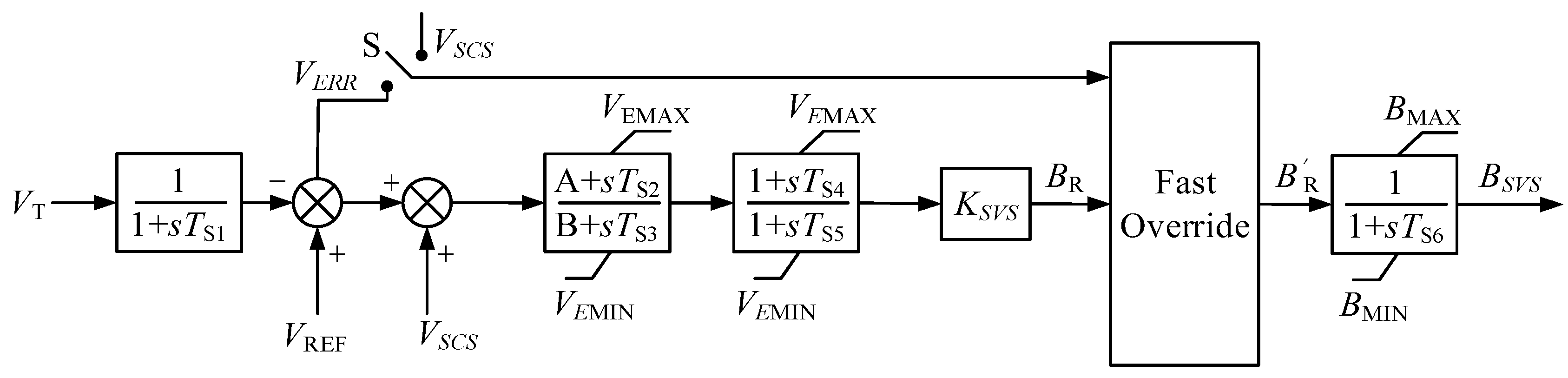
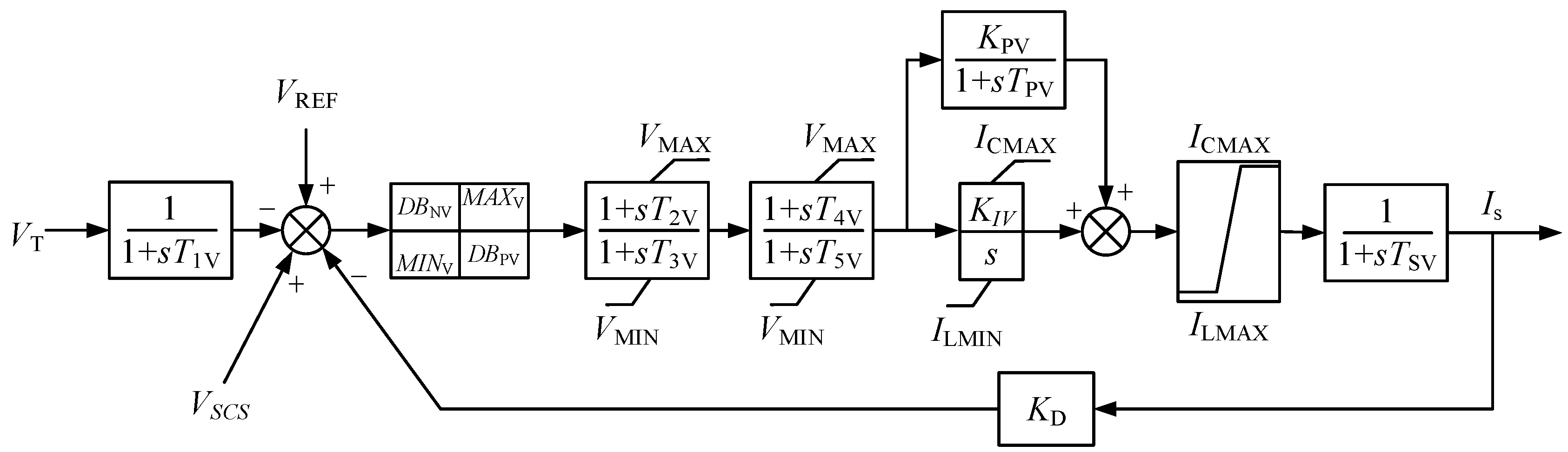
3.1. Basic Model of Dynamic Reactive Power Source Devices

When operating, the control process of an SVC is as follows: The voltage measurement unit first detects the voltage of the controlled bus. After sampling, the measured voltage is compared with the set reference voltage. Through the logical processing stage, the compensation value required to bring the voltage to the set value is calculated. Based on the required reactance, the corresponding control signals for switching TCR and TSC units are generated. The core control model of the SVC in PSD-BPA software (version 5.9.1) is shown in Figure 3. In this model VT is the measured node voltage, VREF is the reference voltage, VERR is the voltage deviation, VSCS is the auxiliary signal voltage, and BSVS is the output reactance value.
When operating, the control process of the STATCOM is as follows: The voltage measurement unit first detects the voltage of the controlled bus. After sampling, the measured voltage is compared with the set reference voltage. Through the logical processing stage, the required current value to compensate the voltage to the set value is calculated and the corresponding triggering pulse signals are output. The core control model of the STATCOM in PSD-BPA software is shown in Figure 4. In this model VT is the measured node voltage, VREF is the reference voltage, VSCS is the auxiliary signal voltage, and Is is the injected current.
The synchronous condenser typically consists of a synchronous motor and an excitation system. It adjusts the excitation current of the system through an automatic voltage regulator (AVR), allowing it to operate in an over-excitation or under-excitation state. In this mode it absorbs or supplies the necessary reactive power to maintain the system’s voltage level. The control model of the synchronous condenser’s FV-type excitation system in PSD-BPA software is shown in Figure 5. In this model UC is the voltage measured after the voltage VT and current IT pass through the reactance XC, VREF is the reference voltage, vs. is the auxiliary signal voltage, and EFD is the output excitation voltage.

3.2. Sensitivity Analysis of Dynamic Reactive Power Source Control Parameters

The control parameters of dynamic reactive power compensation devices directly affect their dynamic response characteristics and the effectiveness of transient overvoltage suppression. To optimize the operational performance of these devices and enhance the adaptability of control strategies, it is necessary to explore the sensitivity of key control parameters to transient overvoltage suppression. In this section, based on the model in the PSD-BPA software, a quantitative analysis is conducted on the control parameters of SVC, STATCOM, and synchronous condensers. Using trajectory sensitivity and parameter perturbation methods the dynamic relationship mechanism of control parameters to transient overvoltage peak values is revealed, high-sensitivity parameters are identified, and the optimization direction for these parameters is clarified, providing theoretical support for the parameter setting of multi-reactive power source collaborative control strategies.
Trajectory sensitivity is an indicator used in power system dynamic analysis to quantify the sensitivity of system state variables, such as voltage, current, and frequency, to small changes in parameters like control parameters, device parameters, or system operating conditions [17]. The trajectory refers to the curve of the state variable’s variation over time. The core of this method is to use mathematical techniques to reveal how parameter changes affect the system’s dynamic response trajectory. Trajectory sensitivity can capture the real-time impact of parameter changes on the system’s transient process rather than just steady-state results. It is particularly suitable for complex scenarios arising from the large-scale integration of new energy sources and power electronic devices in current power systems. Thus, it provides a theoretical basis for parameter optimization, control strategy design, and fault suppression.
The calculation of trajectory sensitivity is based on the state equations of the system’s dynamic model. Let the state equation of the AC–DC hybrid transmission system be as follows:
x ˙ ( t ) = f ( x ( t ) , y ( t ) , u ) 0 = g ( x ( t ) , y ( t ) , u )
where f represents the system state equation; x ( t ) is the system state variable; x ˙ ( t ) is the derivative of the system state variable; y ( t ) is the system algebraic variable; u is the control parameter to be analyzed; and g is the system constraint equation.
Let the trajectory function of the state variables and algebraic variables be as follows:
x ( t ) = Φ x ( u , t ) y ( t ) = Φ y ( u , t )
For a small perturbation Δu on the control parameter u, by performing a Taylor expansion and neglecting higher-order terms the trajectory sensitivity of the state variable x with respect to the control parameter u and the change in the algebraic variable y after the perturbation of parameter u can be derived as follows:
Δ x ( t ) = Φ x ( u 0 , t ) u 0 ( u u 0 ) = x u ( t ) Δ u Δ y ( t ) = Φ y ( u 0 , t ) u 0 ( u u 0 ) = y u ( t ) Δ u
By taking the limit of these variations, we obtain the following trajectory sensitivity:
x u ( t ) lim Δ u 0 Δ x ( t ) Δ u = Φ x ( u 0 + Δ u , t ) Φ x ( u 0 , t ) Δ u y u ( t ) lim Δ u 0 Δ y ( t ) Δ u = Φ y ( u 0 + Δ u , t ) Φ y ( u 0 , t ) Δ u
The solution of trajectory sensitivity includes both the direct method and the perturbation method. The direct method calculates the partial derivative of the state variable with respect to the parameter by solving the adjoint equation or sensitivity differential equations. This method is suitable for linear or weakly nonlinear systems. The perturbation method involves performing multiple simulations with small perturbations of parameters, comparing the trajectories before and after the parameter changes, and calculating the sensitivity value. This method is suitable for complex nonlinear systems or models that cannot be solved analytically. The new energy DC transmission system studied in this paper is characterized by its complex structure and high coupling, making it difficult to achieve an analytical solution using the differential method. Therefore, the perturbation method is chosen for analysis.
The parameter perturbation method is an analytical approach that studies the impact of small changes or “perturbations” in specific parameters of a model or system on the system’s dynamic response [18]. The core idea is to observe the changes in system outputs, such as the transient overvoltage peak, as a result of small local or global changes in parameters. This helps to quantify the sensitivity of the system’s performance to these parameters. By applying local perturbations, the impact of a single parameter can be isolated, avoiding the complexity caused by multiple parameter couplings and making it suitable for complex power system models. It allows for the rapid identification of key control parameters, the recognition of high-sensitivity parameters, and the clarification of their dominant role in transient overvoltage suppression, providing a basis for parameter tuning.
When calculating the trajectory sensitivity of dynamic reactive power compensation control parameters, the trajectory change corresponds to the transient overvoltage peak before and after the perturbation. The transient overvoltage sensitivity to dynamic reactive power compensation control parameters can be defined as follows:
T S T V O _ p a = Δ U T V O ( Δ u ) Δ u / u 0 × 10 3 = U p e a k u 1 U p e a k u 0 u 1 u 0 / u 0 × 10 3
where u 0 represents the initial value of the control parameter; u 1 represents the value of the control parameter after the change; Δ u represents the change in the control parameter; U T V O represents the transient overvoltage peak value; Δ U T V O ( Δ u ) represents the change in the transient overvoltage peak value corresponding to the control parameter change; U p e a k represents the transient overvoltage peak value during system operation; and Δ u / u 0 is used to normalize the change in the parameter so that parameters with different dimensions can be compared on a unified reference scale. A negative sign is introduced to ensure that when the value of this indicator is positive, an increase or decrease in the parameter corresponds to an enhancement or weakening of the transient overvoltage suppression effect.
In practical calculations, trajectory sensitivity analysis is limited to small perturbations of parameters, which may lead to issues such as the initial value of the parameter being in an insensitive range, the initial parameter being too small to compute the magnitude of trajectory sensitivity, or the computed trajectory sensitivity value not effectively representing the parameter’s sensitivity. When parameters vary significantly within a broader range but the initial parameter value lies in a local insensitive region, a new sensitivity indicator must be introduced to efficiently and accurately reflect the strength of the control parameter’s sensitivity over a wide range of values. The additional interval trajectory sensitivity indicator is defined as follows:
I T S T V O _ p a = Δ U T V O ( u max u min ) ( u max u min ) / u 0 × 10 3 = U p e a k u max U p e a k u min u max u min / u 0 × 10 3
where u min and u max are the minimum and maximum adjustment range of the control parameter. Similarly, ( u max u min ) / u 0 is the normalization factor.

3.2.1. SVC Parameter Sensitivity Analysis

For the analysis of SVC parameters in the system shown in Figure 1, eight sets of wind turbines (150 MW each) are configured, with a DC line transmission capacity of 1300 MW. A 300 Mvar SVC device is added to the low-voltage side of the wind turbine step-up transformer. The initial control parameters are set to the default values in the PSD-BPA software and commonly used values in engineering practices.
The initial values of the control parameters to be analyzed, along with their test ranges, are shown in Table 1.
The sensitivity calculation results for the parameters are shown in Table 2.
For the parameter Ts1, both the TSTVO_pa and ITSTVO_pa indicators for blocking and commutation failure are negative, indicating that the adjustment of this parameter is inversely related to transient overvoltage suppression. The larger the parameter, the greater the overvoltage.
For the parameter VEMAX, the ITSTVO_pa indicators for blocking and commutation failure are positive and negative, respectively, indicating that the effect of this parameter adjustment on the two types of transient overvoltage is opposite.
For the parameters Ts2 and Ts4, both the TSTVO_pa and ITSTVO_pa indicators for blocking and commutation failure are positive, indicating that the adjustment of these parameters is directly proportional to transient overvoltage suppression.
For the parameters Ts3 and Ts5, both the TSTVO_pa and ITSTVO_pa indicators for blocking and commutation failure are negative, indicating that the adjustment of these parameters is inversely proportional to transient overvoltage suppression.
For the parameter Ksvs, the TSTVO_pa and ITSTVO_pa indicators for blocking and commutation failure are positive and negative, respectively, indicating that the effect of this parameter adjustment on the two types of transient overvoltage is opposite.
For the parameter DV, the TSTVO_pa and ITSTVO_pa indicators for blocking and commutation failure are negative and positive, respectively, indicating that the effect of this parameter adjustment on the two types of transient overvoltage is opposite.
By comprehensively considering the size of the TSTVO_pa and ITSTVO_pa parameters, as well as whether each parameter’s adjustment consistently affects both types of transient overvoltage, the priority for parameter adjustment is determined as follows: DV > Ts1 > Ts3 > Ksvs > Ts5 > Ts2 > Ts4 > VEMAX. In the process of parameter tuning, particular attention should be given to the regulation of parameters with higher levels of priority.

3.2.2. STATCOM Parameter Sensitivity Analysis

For the analysis of STATCOM parameters in the system shown in Figure 1, eight sets of wind turbines (150 MW each) are configured, with a DC line transmission capacity of 1300 MW. A 300 Mvar STATCOM device is added to the low-voltage side of the wind turbine step-up transformer. The initial control parameters are set to the default values in the PSD-BPA software and commonly used values in engineering practices.
The initial values of the control parameters to be analyzed, along with their test ranges, are shown in Table 3.
VOL_REFH is the reference voltage, SETDATAH is the adjustment coefficient, VOL_HIGH is the threshold for high-voltage ride-through (HVRT) entry judgment, VOL_HIGH_RET is the threshold for HVRT exit judgment, and VOL_HIGH_DELAY is the high-voltage judgment cycle.
The sensitivity calculation results for the parameters are shown in Table 4.
For the parameters VOL_REFH, VOL_HIGH, and VOL_HIGH_DELAY, the TSTVO_pa and ITSTVO_pa indicators for both blocking and commutation failure are negative, indicating that adjusting these parameters is inversely related to transient overvoltage suppression. The larger the parameter, the greater the overvoltage.
For the parameter SETDATAH, both the TSTVO_pa and ITSTVO_pa indicators for blocking and commutation failure are positive, indicating that adjusting this parameter is directly proportional to transient overvoltage suppression.
The parameter VOL_HIGH_RET, which is the threshold voltage for STATCOM to exit HVRT, needs to be analyzed in conjunction with the HVRT entry threshold VOL_HIGH. The larger the offset from the entry threshold voltage, the better it can prevent oscillation and enhance the suppression of transient overvoltage under DC blocking conditions.
By comprehensively considering the size of the TSTVO_pa and ITSTVO_pa parameters, as well as whether each parameter’s adjustment consistently affects both types of transient overvoltage, the priority for parameter adjustment is determined as follows: VOL_REFH > VOL_HIGH > SETDATAH > VOL_HIGH_RET. In the process of parameter tuning, particular attention should be given to the regulation of parameters with higher levels of priority.

3.2.3. Synchronous Condenser Parameter Sensitivity Analysis

For the analysis of synchronous condenser parameters in the system shown in Figure 1, eight sets of wind turbines (150 MW each) are configured, with a DC line transmission capacity of 1300 MW. A 300 Mvar synchronous condenser device is added to the low-voltage side of the wind turbine step-up transformer. The initial control parameters are set to the default values in the PSD-BPA software and commonly used values in engineering practices.
The initial values of the control parameters to be analyzed, along with their test ranges, are shown in Table 5.
The sensitivity calculation results for the parameters are shown in Table 6.
For the parameter TR both the TSTVO_pa and ITSTVO_pa indicators for blocking and commutation failure are negative, indicating that the adjustment of this parameter is inversely related to transient overvoltage suppression.
For the parameters K, T1, T4, KA, and TA the ITSTVO_pa indicators for blocking and commutation failure are opposite in sign, indicating that the effect of adjusting these parameters on the two types of transient overvoltage is opposite.
For the parameter KV both the TSTVO_pa and ITSTVO_pa indicators for commutation failure are positive, indicating that adjusting this parameter is directly proportional to transient overvoltage suppression under commutation failure.
For the parameters T2 and T3 both the TSTVO_pa and ITSTVO_pa indicators for blocking and commutation failure are positive, indicating that adjusting these parameters is directly proportional to transient overvoltage suppression.
By comprehensively considering the size of the TSTVO_pa and ITSTVO_pa parameters, as well as whether each parameter’s adjustment consistently affects both types of transient overvoltage, the priority for parameter adjustment is determined as follows: TR > K > KA > T1 > TA > T4 > T2 > T3 > KV. In the process of parameter tuning, particular attention should be given to the regulation of parameters with higher levels of priority.

4. Multi-Objective Collaborative Control Strategy for Dynamic Reactive Power Sources

Through the sensitivity analysis of control parameters for the three types of dynamic reactive power devices conducted in the previous chapter, it is observed that adjustments to different control parameters have varying degrees of impact on the suppression of transient overvoltages. Moreover, due to the distinct mechanisms and characteristics of the two types of DC disturbances, tuning the control parameters of dynamic reactive power sources to enhance the suppression of one type of transient overvoltage may simultaneously weaken the suppression effectiveness for the other. To address the challenge of regulatory conflicts encountered when improving transient overvoltage suppression performance, this chapter establishes a coordinated optimization control model and designs an improved solution algorithm.

4.1. Collaborative Optimization Control Model for Transient Overvoltage Suppression

4.1.1. Objective Function

In the face of the primary DC disturbances, with the goal of suppressing the corresponding transient overvoltages, the following target function is established to minimize both types of transient overvoltages:
f o b j 1 ( u ) = min [ U TVO _ BL ( u ) ] = min [ U max _ BL ( u ) U stable ( u ) ] f o b j 2 ( u ) = min [ U TVO _ COM ( u ) ] = min [ U max _ COM ( u ) U stable ( u ) ]
where Umax_BL is the peak transient overvoltage after a DC blocking fault; Umax_COM is the peak transient overvoltage after a commutation failure fault; and u is the vector of control parameters to be optimized.
Objective function fobj1 aims to minimize the transient overvoltage after a DC blocking fault, and objective function fobj2 aims to minimize the transient overvoltage after a commutation failure fault. To accurately calculate the transient voltage rise, the peak value of the transient process after the fault is subtracted by the stable value.

4.1.2. Constraints

In addition to optimizing the control parameters to achieve the minimum fitness function, which is the objective function, certain constraints must be set to ensure that the system operates within its normal operating range.
  • System Power Balance Constraint
The most basic and crucial constraint in the power system model is the power balance, which is as follows:
P G i P d i U i j i U j G i j cos θ i j + B i j sin θ i j = 0 Q G i Q d i U i j i U j G i j cos θ i j B i j sin θ i j = 0
where P G i and Q G i are the active and reactive power outputs of the generator at node i; P d i and Q d i are the active and reactive power loads at node i; θ i j , G i j , and B i j are the phase angle difference, conductance, and susceptance between nodes i and j; and U i and U j are the voltages at nodes i and j.
  • System State Variable Constraints
During operation, power, voltage, current, and other state variables are subject to maximum and minimum limits to ensure the model is reasonable and operates in a normal state, which can be expressed as follows:
P G i , max P G i P G i , max Q G i , max Q G i Q G i , max U i , min U i U i , max I i j , min I i j I i j , max
where I i j is the transmission current between branches (i, j).
  • Control Parameter Range Constraints
When adjusting the control parameters, it is important to ensure that the parameters vary within a reasonable range. The upper and lower limits of the control parameters should be set to restrict the size of the search space, which can be expressed as follows:
u min u u max
where umin is the minimum value limit of the control parameters to be optimized; and umax is the maximum value limit of the control parameters to be optimized.

4.2. Collaborative Optimization Control Solution Method

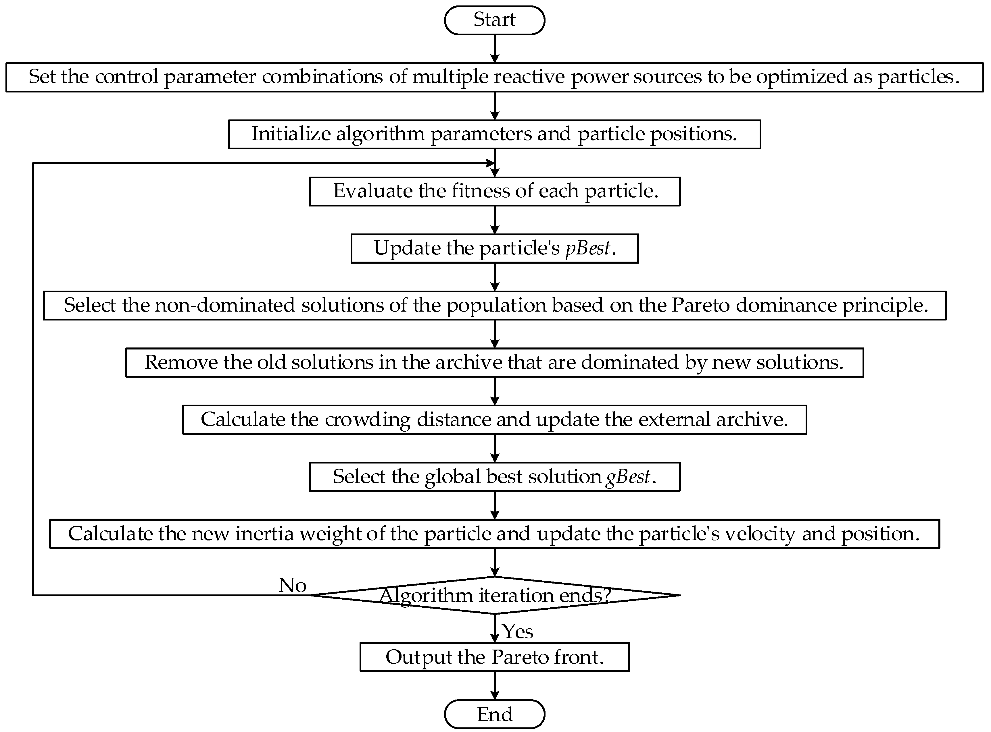
4.2.1. Particle Swarm Optimization Algorithm

Particle swarm optimization (PSO) is inspired by the foraging behavior of birds, where a flock of birds shares collective information to find the optimal destination [19]. In PSO each particle’s position represents a candidate solution to the problem. The quality of each particle’s location in space depends on the fitness of that position in the problem. The position of each particle in the next generation is determined by its velocity vector, which controls the direction and distance of each movement. During flight, the particle will record the best position it has visited, known as pBest, and the group will also update the best position reached by the whole group, referred to as gBest. The velocity of a particle is determined by its current position, its best position, the best position of the group, and its velocity. The core principles of the particle swarm algorithm are described by the following equations:
v i d = w v i d 1 + c 1 r 1 p B e s t i d x i d + c 2 r 2 g B e s t d x i d
x i d + 1 = x i d + v i d
where v i d represents the velocity of the i-th particle during the d-th iteration cycle; x i d represents the position of the i-th particle during the d-th iteration cycle; c 1 is the particle’s cognitive learning factor; c 2 is the particle’s social learning factor; w is the inertia weight of the velocity; p B e s t i d is the personal best of the i-th particle up to the d-th iteration; and g B e s t d is the global best of all particles up to the d-th iteration.

4.2.2. Dynamic Inertia Weight Considering Comprehensive Trajectory Sensitivity

Based on the trajectory sensitivity TSTVO_pa and interval trajectory sensitivity ITSTVO_pa set in the previous chapter, both are considered comprehensively and defined as the comprehensive trajectory sensitivity indicator, which is as follows:
C T S T V O _ p a = T S T V O _ p a + I T S T V O _ p a
By combining the CTSTVOBL_pa values corresponding to both DC blocking and commutation failure we obtain the weight sensitivity indicator Sw_pa for parameter selection and particle update improvement in the dual-objective optimization model, which is as follows:
S w _ p a = C T S T V O B L _ p a + C T S T V O C O M _ p a
where CTSTVOBL_pa is the comprehensive trajectory sensitivity corresponding to the DC blocking fault and CTSTVOCOM_pa is the comprehensive trajectory sensitivity corresponding to the commutation failure fault.
Traditional PSO treats all parameters equally. When the fitness change is small, inertia weight should be increased to promote global search. When the fitness change is large, indicating that optimization has made significant progress, the inertia weight should be decreased to promote local search. The commonly used dynamic inertia weight is as follows [20]:
w i d = w min + ( w max w min ) 1 Δ f i d Δ f max d
where Δ f i d is the change in fitness function value of the current particle at the d-th iteration and Δ f max d is the maximum change in the fitness function of all particles at the d-th iteration.
By introducing sensitivity weight, particles with high sensitivity parameters are given larger adjustment weights. This allows these key parameters to be prioritized for optimization, with computational resources focused on them, thus accelerating convergence during the initial iteration and avoiding ineffective oscillations. As the iteration progresses, the weight should be reduced to help particles converge better and fine-tune the search. This requires combining the sensitivity weight with a time decay function and ensuring normalization of sensitivity. The specific calculation formula is:
w i d = w min + ( w max w min ) 1 Δ f i d Δ f max d 1 + S w _ p a , i m = 1 n S w _ p a , m α k e λ d i t e r
where α k is the initial decay coefficient; λ is the decay rate; iter is the maximum iteration count; and m = 1 n S w _ p a , m is the sum of all weight sensitivities for the parameters to be optimized.
Based on the modified inertia weight formula, the final particle swarm velocity update formula is:
v i d = w i d 1 v i d 1 + c 1 r 1 p B e s t i d x i d + c 2 r 2 g B e s t d x i d

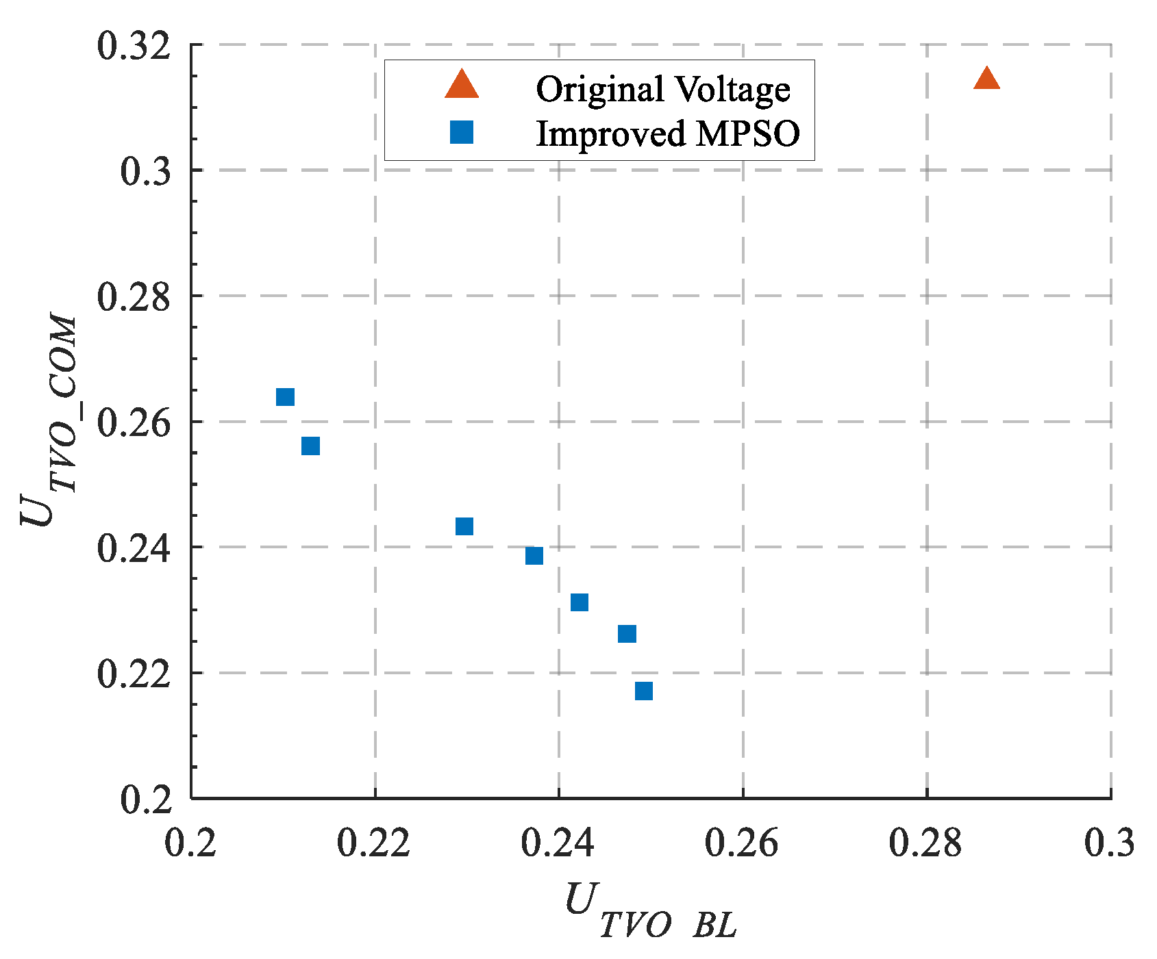
4.2.3. Multi-Objective Optimization and Pareto Front

In multi-objective optimization problems there is often a trade-off between conflicting objective functions. Traditional methods such as the weighted method, goal programming, or hierarchical goal programming rely on prior knowledge to artificially intervene in the objectives (e.g., setting weight coefficients or priorities). Essentially, these methods simplify the multi-objective problem into a single-objective optimization. However, such methods have significant limitations as the choice of weights or priorities is highly subjective and it is difficult to fully reflect the complex nonlinear relationships between objectives, leading to solutions that may be biased toward local or suboptimal regions. Therefore, the Pareto optimality theory is introduced to address the problem. The core idea is to depict the inherent trade-offs between objectives through a non-dominated solution set (i.e., the Pareto front), providing decision-makers with a global solution set without the need for pre-set preferences [21].
In the dual-objective optimization scenario, the Pareto front is defined as the set of Pareto optimal solutions in the objective space that are not dominated by any other solution. Specifically, if two candidate solutions x1 and x2 exist, x1 dominates x2 if and only if x1 is no worse than x2 in all objective functions (i.e., f1(x1) ≤ f1(x2) and f2(x1) ≤ f2(x2)) and strictly better in at least one objective. All candidate solutions that are not dominated by others form the Pareto optimal solution set, and their projection in the objective space forms the Pareto front. The mathematical expression is as follows [22]:
ParetoFront = { ( f 1 ( x ) , f 2 ( x ) ) 2 x Ω ,   x Ω   s . t .   x x }
where is the real number space; Ω is the feasible solution space; and represents the dominant relationship.
The geometric characteristics of the Pareto front reflect the degree of conflict between objectives. The closer the front is to a convex shape, the easier it is to reconcile the objectives; conversely, a non-convex region suggests sharp trade-offs.
In the multi-objective particle swarm optimization (MPSO) algorithm, the algorithm efficiently approximates the Pareto front by dynamically maintaining an external archive storing non-dominated solutions and introducing a diversity preservation mechanism [23]. The particles that are considered Pareto optimal are stored in the archive, and the gBest is selected from the archive to guide the particle swarm, maintaining the breadth of the search.
The global best guide gBest can be selected from the archive based on crowding distance or other density measures to balance solution convergence and distribution. The crowding distance is calculated by quantifying the local density of solutions in the objective space and it is defined as follows [24]:
CrowdingDistance ( x ) = k = 1 2 f k ( x next ) f k ( x prev ) f k max f k min
where x next and x prev are the adjacent solutions sorted by objective value and f k max and f k min are the maximum and minimum values of the k-th objective in the current archive.
This indicator is used to prioritize solutions with larger crowding distances when the archive capacity is exceeded, preventing over-concentration of frontier solutions, maintaining archive manageability, and encouraging solution diversity. Additionally, the particle’s individual best position pBest update follows the dominance relationship: if the new position is not dominated by the original pBest it replaces the original individual best.
Through continuous iterations, the particle swarm gradually converges to and uniformly covers the real Pareto front, providing a set of representative trade-off solutions for multi-objective decision-making.
The flowchart of the MPSO algorithm combined with the Pareto front is shown in Figure 6.

4.3. Case Study Analysis

4.3.1. Equivalent Three-Machine System

In the system shown in Figure 1, eight sets of wind turbines (150 MW each) are configured, with a DC line transmission capacity of 1300 MW. Various types of dynamic reactive power sources are added to the system to simulate the dynamic reactive power source configuration scenarios in actual engineering. A 50 Mvar synchronous condenser is added to the low-voltage side of the wind turbine step-up transformer, a 300 Mvar STATCOM device is added to the low-voltage side of the wind turbine step-up transformer, and a 360 Mvar SVC device is added to the AC bus of the DC converter station at the sending end. The initial control parameters and the upper and lower limits for adjusting the control parameters are set as in the previous chapter.
Before solving the collaborative optimization control model, the relevant algorithm parameters are set as follows: c 1 and c 2 are both 2, w max is 0.9, w min is 0.6, the initial decay coefficient α k is 1.5, the decay rate λ is 2, the population size is 100, and the maximum iteration count is 30. Based on the analysis in the previous chapter, the optimized control parameters selected are Ts1, Ts3 and DV for the SVC; VOL_REFH and VOL_HIGH for the STATCOM; and TR, K and KA for the synchronous condenser.
For comparison, the standard inertia weight MPSO algorithm and the improved MPSO algorithm proposed in this paper are both used to solve the collaborative control model. The two objective functions are added together and the iteration convergence curve of the algorithm is plotted, as shown in Figure 7.
It can be observed that the standard inertia weight MPSO algorithm converges more slowly than the improved MPSO. The standard MPSO requires 19 iterations to converge, while the improved MPSO only requires 13 iterations. Additionally, when converged, the fitness of the improved MPSO algorithm is better than that of the standard inertia weight MPSO.
The solution results of the optimization model are shown in Figure 8.
From the result plot, it can be seen that compared to the initial parameters before optimization, the corresponding transient overvoltage rise for DC blocking and commutation failure are 0.2945 p.u. and 0.2614 p.u., respectively. The Pareto front optimization result after algorithm optimization is significantly lower than the initial transient overvoltage. The DC blocking transient overvoltage can be reduced by more than 0.1 p.u. and the commutation failure transient overvoltage can be reduced by more than 0.05 p.u. Moreover, the improved MPSO algorithm’s Pareto front result is better than the standard inertia weight MPSO, being entirely inside the standard inertia weight MPSO result, further confirming the superiority of the dynamic inertia weight considering comprehensive trajectory sensitivity.
For the selection of Pareto solutions, each solution is better than the initial transient overvoltage before optimization. In practical engineering, an appropriate solution can be selected according to the required transient overvoltage suppression. A point is selected where both transient overvoltages are relatively balanced, with a DC blocking transient overvoltage rise of 0.2135 p.u. and a commutation failure transient overvoltage rise of 0.2119 p.u. The corresponding control parameters are Ts1 for the SVC is 0.01, Ts3 for the SVC is 0.05, and DV for the SVC is 0.42; VOL_REFH for the STATCOM is 1.027 and VOL_HIGH for the STATCOM is 1.086; TR for the synchronous condenser is 2.021, K for the synchronous condenser is 2.30, and KA for the synchronous condenser is 6.42.
The results for both types of transient overvoltages are shown in Figure 9 and Figure 10.
Under this set of control parameters, the DC blocking transient overvoltage is reduced by 0.0810 p.u. and the commutation failure transient overvoltage is reduced by 0.0495 p.u., effectively suppressing the transient overvoltage. In the case of DC blocking faults, optimization primarily focuses on weakening capacitive reactive power accumulation to suppress voltage rise. In contrast, during commutation failure faults the optimization relies more on reactive power support and voltage recovery coordination, thus imposing higher demands on the dynamic response rate. The proposed strategy demonstrates good adaptability under both types of faults, reflecting the general applicability of the model and algorithm.

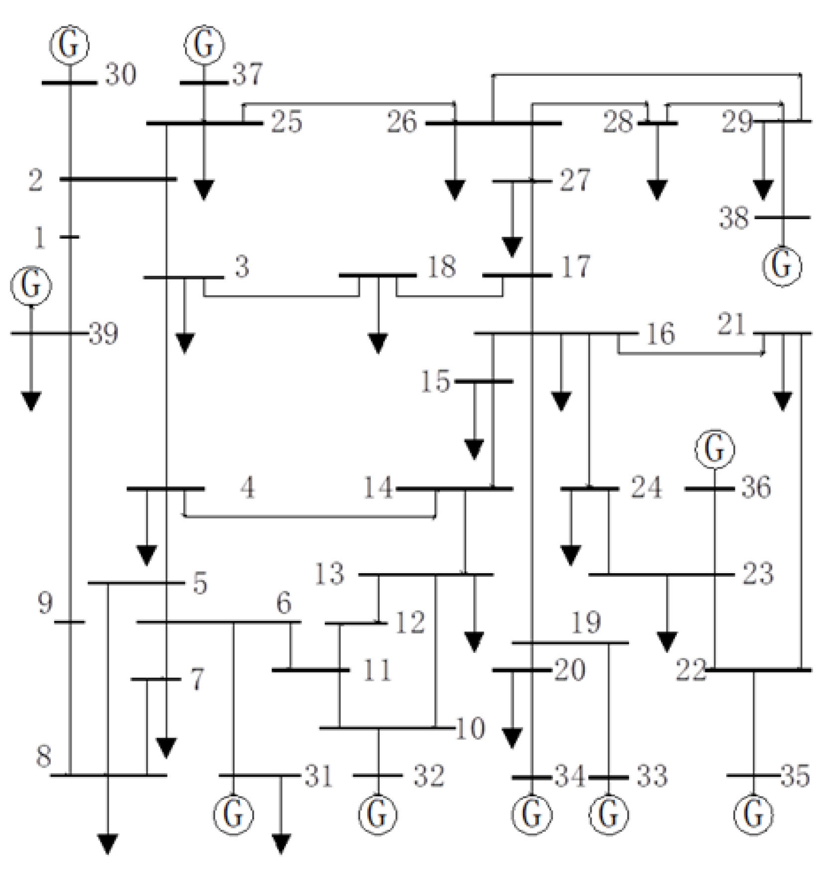
4.3.2. Dual IEEE 39-Bus Hybrid System

To better validate the effectiveness of the designed model and algorithm, two IEEE 39-bus systems are used as the sending-end and receiving-end grids, respectively. A hybrid AC–DC system is established by connecting them via a DC transmission line. The structure of a typical IEEE 39-bus system is shown in Figure 11.
For convenience, the sending-end network is referred to as Area A, and the receiving-end network as Area B. A DC transmission line is established between Node A16 in the sending-end network and Node B8 in the receiving-end network. The DC line is set with a voltage level of ±800 kV and with a transmission power of 5000 MW under bipolar operation. A 3000 MW wind power generator is added at Node A12. Various types of dynamic reactive power sources are incorporated into the system to simulate actual engineering scenarios of dynamic reactive power source configurations. An SVC with a total capacity of 720 Mvar is installed at the wind farm gathering station, a STATCOM with a total capacity of 450 Mvar is placed at the low-voltage side of the wind turbine step-up transformer, and a synchronous condenser with a total capacity of 600 Mvar is added at the AC bus of the DC converter station. The initial control parameters and their upper and lower adjustment limits are set as described in the previous chapter.
Based on the analysis in the previous chapter, the optimized control parameters selected are Ts1, Ts3, and DV for the SVC; VOL_REFH and VOL_HIGH for the STATCOM; and TR, K and KA for the synchronous condenser. The Pareto front results after model solving are shown in Figure 12.
From the result graph it can be observed that compared to the initial parameters before optimization, where the DC blocking transient overvoltage and DC commutation failure transient overvoltage rise were 0.2865 p.u. and 0.3142 p.u., respectively, the Pareto front optimization results after algorithm optimization are significantly smaller than the initial transient overvoltage. The DC blocking transient overvoltage can be reduced by up to 0.07 p.u. and the commutation failure transient overvoltage can be reduced by up to 0.09 p.u.
Regarding the selection of Pareto solutions, each solution is superior to the initial transient overvoltage before optimization. In practical engineering an appropriate solution can be selected according to specific needs and the corresponding control parameters can be applied to achieve effective transient overvoltage suppression. Two solutions, where both transient overvoltages are relatively balanced, are selected, one where the DC blocking transient overvoltage rise is 0.2373 p.u., and the other where the commutation failure transient overvoltage rise is 0.2386 p.u. The corresponding control parameters are for the SVC, Ts1 = 0.01, Ts3 = 0.14, and DV = 0.37; for the STATCOM, VOL_REFH = 1.046 and VOL_HIGH = 1.113; and for the synchronous condenser, TR = 1.632, K = 17.53, and KA = 4.87.
The transient overvoltage results under these control parameters are shown in Figure 13 and Figure 14.
With this set of control parameters, the DC blocking transient overvoltage is reduced by 0.0492 p.u. and the DC commutation failure transient overvoltage is reduced by 0.0756 p.u., effectively suppressing transient overvoltage. Under coordinated optimization control the dynamic reactive power sources’ response timing and magnitude are coordinated within the system, effectively mitigating the reactive power redundancy caused by DC blocking and the reactive power insufficiency caused by commutation failure, thereby suppressing the amplitude fluctuations of transient overvoltage. The optimization demonstrates good adaptability across different fault scenarios, highlighting the broad applicability of the proposed method to complex fault dynamic characteristics.

5. Conclusions

This paper addresses the issue of transient overvoltages induced by DC blocking and commutation failures in new energy DC transmission systems. In response to the limitations of traditional dynamic reactive power control strategies—particularly in terms of multi-fault compatibility, parameter optimization, and coordinated control of multiple devices—a systematic modeling, analysis, and optimization approach is proposed. By revealing the fault dynamic mechanisms, quantifying the influence of control parameters, and innovating coordinated optimization strategies, a new dynamic reactive power collaborative control system targeting multi-fault scenarios is developed. The research outcomes provide a theoretical foundation and practical pathway for enhancing transient voltage stability, optimizing reactive power resource configuration, and improving control in DC transmission systems under high penetration of renewable energy, thereby contributing significantly to the safe and efficient operation of modern power systems. Specifically:
  • A typical system model for renewable energy transmission via DC lines is established. The formation process of transient overvoltages under DC blocking and commutation failure faults is analyzed, and the influence of dynamic reactive power imbalance on voltage evolution is elucidated.
  • Based on trajectory sensitivity analysis and parameter perturbation methods, the impacts of key control parameters of dynamic reactive power devices on transient overvoltages under different faults are systematically quantified. Highly sensitive parameters under multiple fault conditions are identified, leading to a parameter prioritization framework that provides a solid theoretical basis for fine-grained, coordinated control of multiple devices.
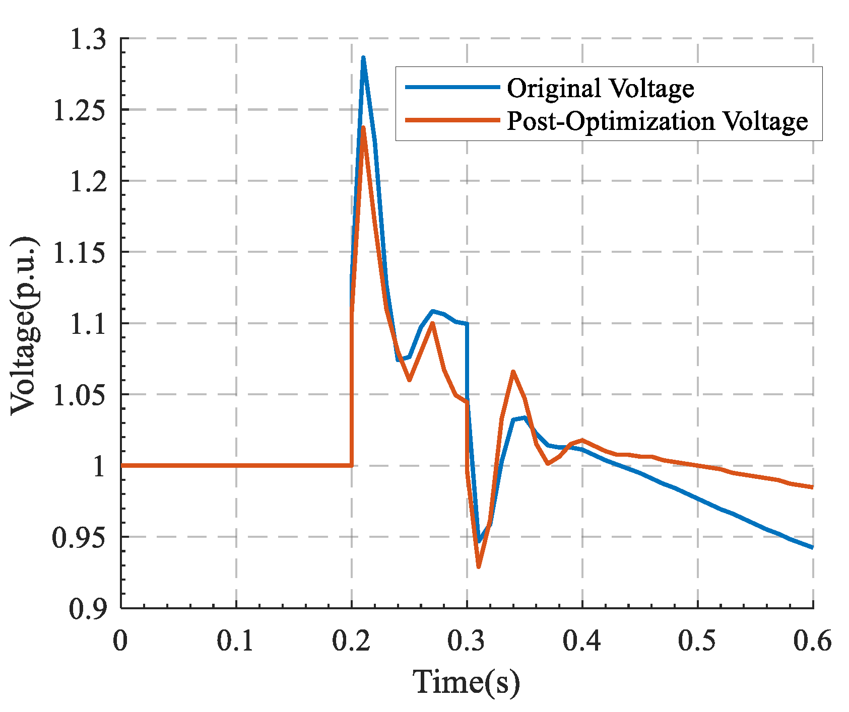
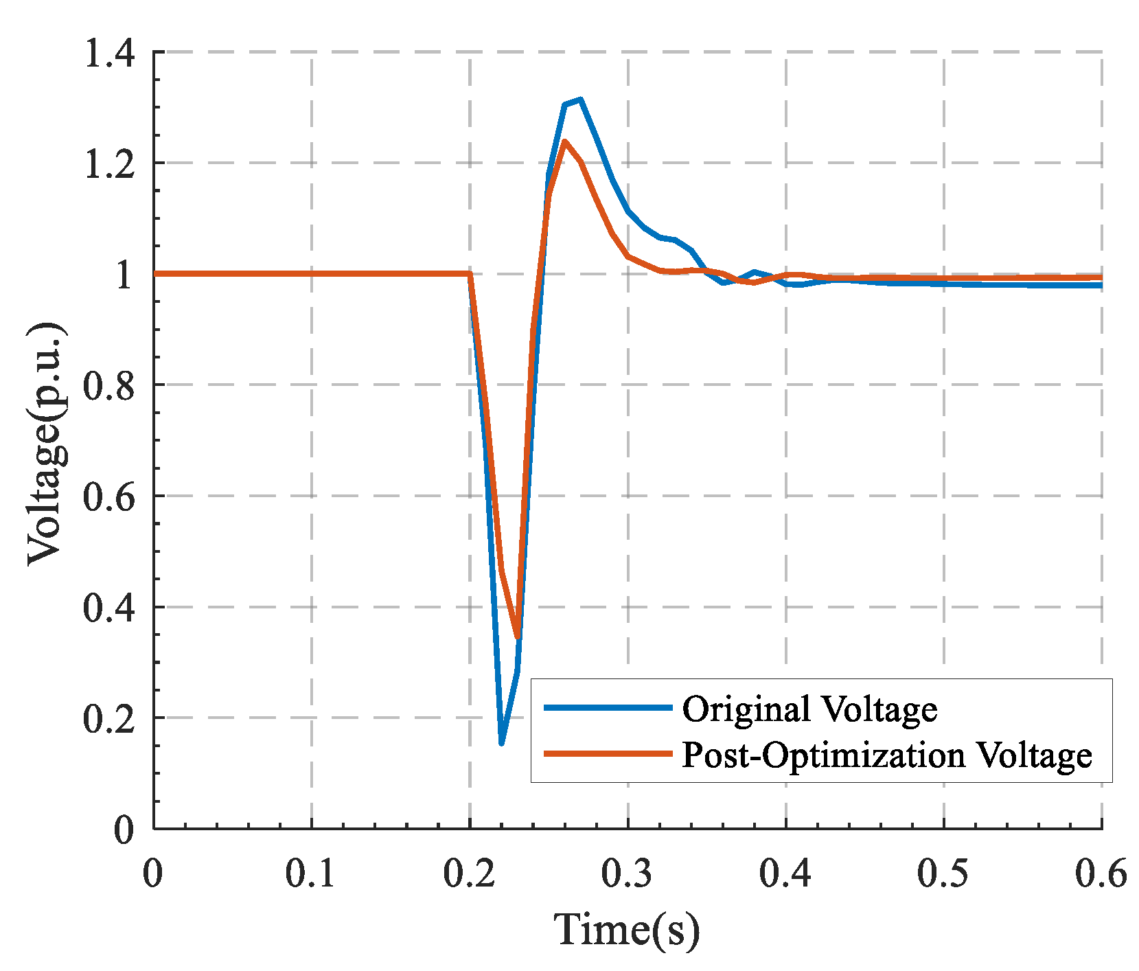
  • A multi-objective coordinated optimization model for multiple reactive power devices is constructed to simultaneously address the suppression requirements of different fault types. A novel optimization algorithm integrating comprehensive trajectory sensitivity with a dynamic inertia weight particle swarm optimization method is proposed, which is combined with Pareto front theory to achieve global optimization of control parameters and coordination among multiple objectives. This significantly enhances the overall dynamic response capabilities of reactive power devices and improves system voltage stability.

Author Contributions

Conceptualization, S.S. and D.C.; methodology, Z.Y.; software, Z.Y.; validation, Z.L. and X.T.; formal analysis, Y.S.; investigation, X.T.; resources, D.C. and Z.L.; data curation, Z.Y. and Y.S.; writing—original draft preparation, Z.Y., S.S. and D.C.; writing—review and editing, Z.Y., S.S. and G.Z.; visualization, X.T. and G.Z.; supervision Z.L. and Y.S.; project administration, S.S.; funding acquisition S.S. All authors have read and agreed to the published version of the manuscript.

Funding

This research was funded by Chinese Academy of Engineering Strategic Research and Advisory Project (JL2024-13) and the Jilin University Teaching Research Project (2023CGP009).

Data Availability Statement

Data are contained within the article.

Conflicts of Interest

The authors declare no conflicts of interest.

References

  1. Harrison, A.; Alombah, N.H.; Kamel, S.; Ghoneim, S.S.M.; El Myasse, I.; Kotb, H. Towards a Simple and Efficient Implementation of Solar Photovoltaic Emulator: An Explicit PV Model Based Approach. Eng. Proc. 2023, 56, 261. [Google Scholar] [CrossRef]
  2. El Myasse, I.; El Magri, A.; Watil, A.; Mansouri, A.; Kissaoui, M.; Ouabi, H.; Blouh, F.E. Enhancing Wind Power Plant Integration Using a T-NPC Converter with DR-HVDC Transmission Systems. IFAC-PapersOnLine 2024, 58, 472–477. [Google Scholar] [CrossRef]
  3. Feng, N.; Feng, Y.; Su, Y.; Zhang, Y.; Niu, T. Dynamic Reactive Power Optimization Strategy for AC/DC Hybrid Power Grid Considering Different Wind Power Penetration Levels. IEEE Access 2024, 12, 187471–187482. [Google Scholar] [CrossRef]
  4. Adireddy, R.; Deepak, B.S.; Ravindra, M.; Ramachandra Murthy, K.V.S. Study of Different Techniques to Mitigate Temporary Overvoltage in Photovoltaic System. Mater. Today Proc. 2022, 56, 3222–3226. [Google Scholar] [CrossRef]
  5. Mohseni, M.; Masoum, M.A.S.; Islam, S.M. Low Voltage Ride-through of DFIG Wind Turbines Complying with Western-Power Grid Code in Australia. In Proceedings of the 2011 IEEE Power and Energy Society General Meeting, Detroit, MI, USA, 24–28 July 2011; pp. 1–8. [Google Scholar]
  6. Amin, M.; Molinas, M. Understanding the Origin of Oscillatory Phenomena Observed Between Wind Farms and HVdc Systems. IEEE J. Emerg. Sel. Top. Power Electron. 2017, 5, 378–392. [Google Scholar] [CrossRef]
  7. Liang, W.; Shen, C.; Sun, H.; Xu, S. Overvoltage Mechanism and Suppression Method for LCC-HVDC Rectifier Station Caused by Sending End AC Faults. IEEE Trans. Power Deliv. 2024, 39, 1299–1302. [Google Scholar] [CrossRef]
  8. Yin, C.; Li, F. Reactive Power Control Strategy for Inhibiting Transient Overvoltage Caused by Commutation Failure. IEEE Trans. Power Syst. 2021, 36, 4764–4777. [Google Scholar] [CrossRef]
  9. Wang, Y.; Zhu, J.; Li, Y.; Hu, J.; Ma, S.; Wang, T. Transient Overvoltage Suppression of LCC-HVDC Sending-end System Based on DC Current Control Optimisation. IET Energy Syst. Integr. 2024, 6, 182–195. [Google Scholar] [CrossRef]
  10. Mannen, T.; Wada, K. Overvoltage Suppression in Initial Charge Control for DC Capacitor Using Multiple Leg Short-Circuits with SiC-MOSFETs in Power Converters. IEEE Open J. Power Electron. 2023, 4, 703–715. [Google Scholar] [CrossRef]
  11. Maruta, H.; Hoshino, D. Transient Response Improvement of Repetitive-Trained Neural Network Controlled DC-DC Converter with Overcompensation Suppression. In Proceedings of the IECON 2019—45th Annual Conference of the IEEE Industrial Electronics Society, Lisbon, Portugal, 14–17 October 2019; Volume 1, pp. 2088–2093. [Google Scholar]
  12. Hamdan, I.; Ibrahim, A.; Noureldeen, O. Modified STATCOM Control Strategy for Fault Ride-through Capability Enhancement of Grid-Connected PV/Wind Hybrid Power System during Voltage Sag. SN Appl. Sci. 2020, 2, 364. [Google Scholar] [CrossRef]
  13. Guo, C.; Wang, Z.; Mu, Z.; Yin, H. Research on Power Frequency Overvoltage and Reactive Power Compensation of Transmission Lines Considering New Energy Access. In Proceedings of the 2024 9th Asia Conference on Power and Electrical Engineering (ACPEE), Shanghai, China, 11–13 April 2024; pp. 1888–1892. [Google Scholar] [CrossRef]
  14. Wu, D.; Ma, B.; Du, Y.; Zhao, T.; Jia, Z. Dynamic Reactive Power Allocation with Multi-Source Coordination in the AC Collecting System of the Large Scale Renewable Energy Base. In Proceedings of the 2024 4th Power System and Green Energy Conference (PSGEC), Shanghai, China, 22–24 August 2024; pp. 581–585. [Google Scholar] [CrossRef]
  15. Manuela Monteiro Pereira, R.; Manuel Machado Ferreira, C.; Maciel Barbosa, F. Comparative Study of STATCOM and SVC Performance on Dynamic Voltage Collapse of an Electric Power System with Wind Generation. IEEE Lat. Am. Trans. 2014, 12, 138–145. [Google Scholar] [CrossRef]
  16. Pathak, A.K.; Sharma, M.P.; Gupta, M. Effect on Static and Dynamic Reactive Power in High Penetration Wind Power System with Altering SVC Location. In Proceedings of the 2016 IEEE 6th International Conference on Power Systems (ICPS), New Delhi, India, 4–6 March 2016; pp. 1–6. [Google Scholar]
  17. Xu, Y.; Dong, Z.Y.; Zhao, J.; Xue, Y.; Hill, D.J. Trajectory Sensitivity Analysis on the Equivalent One-Machine-Infinite-Bus of Multi-Machine Systems for Preventive Transient Stability Control. IET Gener. Transm. Distrib. 2015, 9, 276–286. [Google Scholar] [CrossRef]
  18. Umer, M.; Olejnik, P. Approximate Analytical Approaches to Nonlinear Differential Equations: A Review of Perturbation, Decomposition and Coefficient Methods in Engineering. Arch. Computat. Methods Eng. 2025, in press. [Google Scholar] [CrossRef]
  19. Kennedy, J.; Eberhart, R. Particle Swarm Optimization. In Proceedings of the ICNN’95—International Conference on Neural Networks, Perth, WA, Australia, 27 November–1 December 1995; pp. 1942–1948. [Google Scholar]
  20. Zdiri, S.; Chrouta, J.; Zaafouri, A. Cooperative Multi-Swarm Particle Swarm Optimization Based on Adaptive and Time-Varying Inertia Weights. In Proceedings of the 2021 IEEE 2nd International Conference on Signal, Control and Communication (SCC), Tunis, Tunisia, 20–22 December 2021; pp. 200–207. [Google Scholar]
  21. Giagkiozis, I.; Fleming, P.J. Pareto Front Estimation for Decision Making. Evol. Comput. 2014, 22, 651–678. [Google Scholar] [CrossRef] [PubMed]
  22. Tušar, T.; Filipič, B. Visualization of Pareto Front Approximations in Evolutionary Multiobjective Optimization: A Critical Review and the Prosection Method. IEEE Trans. Evol. Comput. 2015, 19, 225–245. [Google Scholar] [CrossRef]
  23. Honghai, K.; Fuqing, S.; Yurui, C.; Kai, W.; Zhiyi, H. Reactive Power Optimization for Distribution Network System with Wind Power Based on Improved Multi-Objective Particle Swarm Optimization Algorithm. Electr. Power Syst. Res. 2022, 213, 108731. [Google Scholar] [CrossRef]
  24. Raquel, C.R.; Naval, P.C. An Effective Use of Crowding Distance in Multiobjective Particle Swarm Optimization. In Proceedings of the 7th Annual Conference on Genetic and Evolutionary Computation, Washington, DC, USA, 25–29 June 2005; Association for Computing Machinery: New York, NY, USA, 2005; pp. 257–264. [Google Scholar]
Figure 1. Equivalent system for wind power transmission via DC.
Energies 18 02349 g001
Figure 2. Sending end equivalent circuit model.
Energies 18 02349 g002
Figure 3. SVC control model.
Energies 18 02349 g003
Figure 4. STATCOM control model.
Energies 18 02349 g004
Figure 5. Control model of synchronous condenser excitation system.
Energies 18 02349 g005
Figure 6. Flowchart of MPSO algorithm combined with Pareto front.
Energies 18 02349 g006
Figure 7. Convergence curve of collaborative control model.
Energies 18 02349 g007
Figure 8. Pareto front results of collaborative control model.
Energies 18 02349 g008
Figure 9. DC blocking transient overvoltage after collaborative control.
Energies 18 02349 g009
Figure 10. Commutation failure transient overvoltage after collaborative control.
Energies 18 02349 g010
Figure 11. Structure of a typical IEEE 39-bus system.
Energies 18 02349 g011
Figure 12. Pareto front results of collaborative control model.
Energies 18 02349 g012
Figure 13. DC blocking transient overvoltage after collaborative control.
Energies 18 02349 g013
Figure 14. Commutation failure transient overvoltage after collaborative control.
Energies 18 02349 g014
Table 1. SVC initial parameters and range.
Parameter NameInitial ValueRange
Ts1 Filter Time Constant (s)0.02(0.00, 0.20)
VEMAX Maximum Voltage Deviation (p.u.)1.16(0.70, 1.30)
Ts2 First Stage Lead Time Constant (s)0.10(0.00, 1.40)
Ts3 First Stage Lag Time Constant (s)0.10(0.01, 1.50)
Ts4 Second Stage Lead Time Constant (s)1.00(0.00, 8.00)
Ts5 Second Stage Lag Time Constant (s)1.00(0.10, 4.90)
Ksvs Continuous Control Gain4.46(0.50, 9.50)
DV Voltage Deviation (p.u.)0.10(0.01, 0.40)
Table 2. SVC parameter sensitivity calculation results.
Parameter NameBL TSTVO_paBL ITSTVO_paCOM TSTVO_paCOM ITSTVO_pa
Ts1−9.40−6.67−38.40−6.55
VEMAX0.000.580.00−0.58
Ts21.600.419.901.00
Ts3−8.50−3.42−4.30−7.00
Ts42.200.717.200.99
Ts5−2.00−1.081.00−1.69
Ksvs2.682.68−1.78−1.49
DV−26.75−7.494.256.85
Table 3. STATCOM initial parameters and range.
Parameter NameInitial ValueRange
VOL_REFH1.10(0.80, 1.30)
SETDATAH5.00(0.00, 20.00)
VOL_HIGH1.10(1.00, 1.30)
VOL_HIGH_RET1.1(1.00, 1.30)
VOL_HIGH_DELAY0(0.00, 5.00)
Table 4. STATCOM parameter sensitivity calculation results.
Parameter NameBL TSTVO_paBL ITSTVO_paCOM TSTVO_paCOM ITSTVO_pa
VOL_REFH−314.60−450.560.00−125.40
SETDATAH14.5029.130.0014.25
VOL_HIGH−88.00−50.600.00−30.80
VOL_HIGH_RET//0.000.00
VOL_HIGH_DELAY−3.20−0.32−16.80−1.68
Table 5. Synchronous condenser initial parameters and range.
Parameter NameInitial ValueRange
TR Regulator Input Filter Time Constant (s)0.02(0.01, 2.00)
K Regulator Gain56.25(1.00, 70.00)
KV Proportional Integral1.00(0.00, 10.00)
T1 First Stage Lead Time Constant (s)1.00(0.10, 10.00)
T2 First Stage Lag Time Constant (s)10.00(0.20, 20.00)
T3 Second Stage Lead Time Constant (s)0.04(0.01, 1.00)
T4 Second Stage Lag Time Constant (s)0.03(0.01, 1.00)
KA Voltage Regulator Gain14.20(1.00, 20.00)
TA Voltage Regulator Amplifier Time Constant (s)0.02(0.01, 1.00)
Table 6. Synchronous condenser parameter sensitivity calculation results.
Parameter NameBL TSTVO_paBL ITSTVO_paCOM TSTVO_paCOM ITSTVO_pa
TR0.000.00−96.00−16.38
K0.002.53−2.25−28.04
KV0.000.000.100.03
T10.000.12−1.50−2.75
T20.000.102.502.12
T30.000.012.400.26
T40.00−0.070.000.43
KA0.001.20−2.13−23.02
TA0.00−0.05−0.200.64
Disclaimer/Publisher’s Note: The statements, opinions and data contained in all publications are solely those of the individual author(s) and contributor(s) and not of MDPI and/or the editor(s). MDPI and/or the editor(s) disclaim responsibility for any injury to people or property resulting from any ideas, methods, instructions or products referred to in the content.

