Article

Modeling Ecological Risk in Bottom Sediments Using Predictive Data Analytics: Implications for Energy Systems

1
Faculty of Management, Lublin University of Technology, 20-618 Lublin, Poland
2
Faculty of Environmental Engineering, Lublin University of Technology, 20-618 Lublin, Poland
3
Faculty of Agrobioengineering, University of Life Sciences in Lublin, 20-950 Lublin, Poland
*
Author to whom correspondence should be addressed.
Energies 2025, 18(9), 2329; https://doi.org/10.3390/en18092329
Submission received: 31 March 2025 / Revised: 29 April 2025 / Accepted: 30 April 2025 / Published: 2 May 2025
(This article belongs to the Special Issue Sustainable Energy, Environment and Low-Carbon Development)

Abstract

:
Sediment accumulation in dam reservoirs significantly impacts hydropower efficiency and infrastructure sustainability. Bottom sediments often contain heavy metals such as Cr, Ni, Cu, Zn, Cd, and Pb, which can pose ecological risks and affect water quality. Moreover, excessive sedimentation reduces reservoir capacity, increases turbine wear, and raises operational costs, ultimately hindering energy production. This study examined the ecological risk of heavy metals in bottom sediments and explored predictive approaches to support sediment management. Using 27 sediment samples from Zemborzyce Lake, the concentrations of selected heavy metals were measured at two depths (5 cm and 30 cm). Ecological risk index (ERI) values for the deep layer were predicted based on surface data using artificial neural networks (ANNs) and multiple linear regression (MLR). Both models showed a high predictive accuracy, demonstrating the potential of data-driven methods in sediment quality assessment. The early identification of high-risk areas allows for targeted dredging and optimized maintenance planning, minimizing disruption to dam operations. Integrating predictive analytics into hydropower management enhances system resilience, environmental protection, and long-term energy efficiency.

1. Introduction

Bottom sediments have been shown to play a pivotal role in the functioning of reservoirs utilized for hydropower production. Their excessive accumulation has been demonstrated to result in a reduction in the usable capacity of reservoirs, thereby directly impacting the efficiency of water retention and the production capacity of hydropower plants. The sedimentation process has also been observed to cause the silting of turbine inlets, increasing the risk of damage to these components, as well as the costs of operation and maintenance of energy infrastructure [1].
Sediments are important for the long-term process of the accumulation of pollutants in aquatic ecosystems. They adsorb nutrients, organic and inorganic compounds, pathogens, microplastics, and heavy metals [2,3,4]. The accumulation of heavy metals in bottom sediments represents a significant challenge to ecosystem health and poses a risk to energy infrastructure, particularly in hydropower systems. The presence of metals can contribute to the corrosion of dam components, reduce reservoir capacity through sedimentation, and impede the operation of turbines and water intakes [5].
The metal content in sediments may vary depending on the depth of the water body. At great depths, the pressure and temperature can promote the formation of inorganic compounds. According to studies, the concentrations of metals in the surface layers of sediments are higher than those in the deeper layers of water reservoirs [6].
Hossain et al. (2007) demonstrated that the heavy metal concentrations in sediment core samples decrease with depth, suggesting the possibility of the desorption or release of heavy metals from anoxic bottom layers [7]. The sedimentary profile at different depths generally reflects different periods. The deeper the sediment layer, the older it is, representing various geological periods, environmental changes, and even human activity. Studying sediments at different depth levels can be laborious, time-consuming, and sometimes impossible due to technical difficulties and changing weather conditions. Therefore, it is necessary to forecast the value of bottom sediments at various depths.
Techniques like atomic absorption spectroscopy (AAS) and inductively coupled plasma atomic emission spectroscopy (ICP-OES) are widely utilized for the measurement of total heavy metal concentrations, representing the standard in spectroscopic analysis methods [8]. Prior to spectroscopic analysis, sediment samples undergo digestion using aqua regia (a mixture of hydrochloric and nitric acid), hydrofluoric acid, peroxide, or hydrogen hypochlorite at elevated temperatures; alternatively, the microwave extraction method is employed. However, the presence of metal silicates in sediments poses a challenge to metal extraction, as they are difficult to decompose [9]. A notable limitation in measuring total metal concentrations is the oversight of the fact that the toxicity of heavy metals, like chromium, can vary depending on their chemical forms [10]. Additionally, the analysis of heavy metals in sediments encounters challenges due to the presence of clay, which can absorb heavy metal ions and change their characteristics. To address this issue, extraction techniques are employed, including Tessier’s method, the simultaneous extractable metal–acid volatile sulfides (SEM-AVS) method, and the HCl acid extraction method. Particularly, the SEM method is complex due to the need for adjustments for over- or underfractions, which result from intricate chemical interactions such as metal chelate formation and adsorption. This method also demands the meticulous management of sample quantities, further contributing to its complexity [11].
The techniques described have limitations, as they are expensive, time-consuming, require the use of chemicals, and must be performed by experienced technicians. Further research should focus on identifying and developing methods that are effective, environmentally sustainable, and economically accessible [12]. The goal of this study was to forecast the ecological risk index for deeper strata of bottom sediments. The ecological risk index serves as a tool to assess the potential hazard posed by heavy metals present in these sediments to aquatic ecosystems. It is a comprehensive indicator that not only accounts for the concentrations of different metals, but also evaluates their toxicity and the likelihood of bioaccumulation in living organisms. This approach provides a more nuanced understanding of the environmental impact of heavy metals, offering insights into both immediate and long-term risks to aquatic life and ecosystems [13]. The proposed modelling approach has the capacity to provide information on sediment management strategies and environmental risk mitigation in energy-relevant aquatic systems. By identifying areas of increased ecological risk, it facilitates targeted remediation and helps to protect both aquatic life and hydropower infrastructure [14].

1.1. Literature Review

Artificial intelligence (AI) has emerged as a pivotal instrument in addressing complex environmental challenges, particularly through its capacity for precise forecasting of hydrometeorological and geochemical variables, including precipitation [15], groundwater levels [16], water quality parameters [17], pollutant concentrations [18], and soil moisture content [19], as well as in elucidating the interdependencies between groundwater dynamics and meteorological conditions [16].
Given the wide range of factors influencing sediment characteristics, machine learning (ML) has emerged as an essential tool in capturing the complexity of these interactions. The versatility of ML algorithms has allowed researchers to address a diverse array of tasks, such as the measurement of sediment particle velocities above sandy and rippled substrates [20], reservoir classification [21], the simulation of the spatio-temporal evolution of reservoir dynamics [22], and the forecasting of cyanotoxins’ presence in reservoirs [23].
In the last twenty years, various artificial intelligence methodologies have been employed for the emulation of elevated levels of heavy metals, such as artificial neural networks, support vector machines (SVMs), and response surface methodology (RSM) [24].
El Chaal and Aboutafail (2022) employed a combination of multiple regression and artificial neural network methodologies for the purpose of forecasting the levels of heavy metals (specifically zinc, boron, and manganese) in the surface water within the Oued Inaouen catchment area. This prediction was based on various physicochemical parameters, including pH, EC, temperature, total dissolved solids, oxidation reduction potential, bicarbonate, calcium carbonate, magnesium, sodium, potassium, chloride, calcium, sulfate sulfur, nitrate nitrogen, phosphorus, and ammonium nitrogen. The ANN-based prediction models were found to be more accurate than the MLR-based ones. The R2 values for boron, manganese, and zinc were obtained using MLR and the ANN. The values assigned to the multiple linear regression model were 0.17, 0.22, and 0.4 correspondingly, whereas the values attributed to the artificial neural network were 0.997, 0.998, and 0.999. In order to enhance the precision of forecasting, a neural network architecture consisting of three layers (input layer, hidden layer, and output layer) was implemented, incorporating specific quantities of nodes for each metal (15 for zinc, 11 for manganese, and 8 for boron) [25].
Manssouri et al. (2014) predicted the concentrations of heavy metals such as Zn, Cu, and Mn in Alboran Sea sediment layers of varying Holocene depths using the ANN MLP-type RNA and MLR. The input data included bathymetric depth, the percentage of sand, fines below 40 microns, the percentage of CaCO3, the percentage of illite, the percentage of smectite, and the percentage of kaolinite + chloite. The MLP-ANN model achieved higher correlation indices (0.88) compared to the MLR models, which only reached values ranging from 0.266 to 0.710. This suggests that nonlinear data processing methods, like neural networks, may be more suitable for modeling complex environmental relationships than traditional linear methods [26].
Abdakkaoui and Badaoui (2014) conducted a comparative analysis between MLR and an ANN for the purpose of estimating the concentrations of four heavy metals (Cd, Cr, Cu, and Pb) based on the physicochemical characteristics of sediments (including organic matter, moisture, fine fraction, pH, CaCO3, carbon, and phosphorus in the sediment, as well as suspended matter in the water column) within the Beht River catchment in Morocco. The research revealed that the ANN exhibited a superior performance compared to MLR in the prediction of heavy metal concentrations in the sediments. The results from the MLR approach indicated coefficients of determination ranging from R2 = 0.26 for Cd to R2 = 0.83 for Cr, while intermediary values were observed for Cu (R2 = 0.55) and Pb (R2 = 0.67). Conversely, the ANN technique demonstrated notably enhanced outcomes, achieving coefficients of determination of R2 = 0.88 for Cd, R2 = 0.93 for Cr, R2 = 0.96 for Cu, and R2 = 0.80 for Pb. These findings underscore the heightened predictive efficacy of the ANN method in contrast to the MLR method [27].
Bhagat et al. (2021) compared the performance of extreme gradient tree boosting (XGBoost) with that of three other artificial intelligence models (ANN, SVM, and RF) in predicting the Pb content in bay sediments in Queensland. The input variables included the concentrations of 20 metals. XGBoost was found to be the most reliable and flexible algorithm for predicting nonlinear and complex behavior. However, experience is required to train the model due to the higher tuning requirements necessary to achieve a significantly improved performance [12].
Venkatramanan et al. (2017) utilized an artificial neural network to predict the metal content in water, with the metal contents in sediments serving as input data. The findings of the study revealed that the artificial neural network exhibited a high level of precision, as evidenced by the coefficients of determination (R2), which varied between 0.61 and 0.97 [28].

1.2. Problem Statement

The utilization of an ANN and MLR to predict heavy metals is based on the physical and chemical parameters of sediments, environmental conditions, and other anthropogenic factors. Studies in this area commonly concentrate on individual heavy metals or the overall properties of sediments, while neglecting the heterogeneity present in sediment layers. No studies have been conducted on predicting the metal concentrations in different layers of bottom sediments using machine learning models. Machine learning models have varying architectures and parameters, depending on the type of data and problem they are applied to. More complex models may be overfitted to training data, resulting in poor forecasting properties on data they were not trained on. The most frequently used machine learning model is multiple regression. This method is preferred for its simplicity and interpretability, and is particularly useful when the relationships between variables are linear or nearly linear. Neural network models are typically selected when the relationship among input data is nonlinear or difficult to explain.
Given the increasing complexity and scale of environmental challenges, data-driven approaches have become indispensable in advancing the understanding and management of ecological risks.
Conventional methodologies, predicated exclusively on the surface monitoring of the metal content in bottom sediments, have proven to be inadequate. The necessity of monitoring sediments is predicated on the understanding that the presence of heavy metals in sediments has been demonstrated to increase the risk of the corrosion and abrasion of turbine components and the clogging of water inlets. This results in the accelerated wear of components, and in extreme cases, may lead to serious system failures [1]. The advent of contemporary predictive models has engendered a paradigm shift in the field of geology, enabling the analysis of deeper layers of sediments. This advancement has facilitated the identification of areas that are particularly susceptible to risk. Predictive models have been shown to be an effective tool for the forecasting of ecological and technical risks associated with bottom sediments in the context of the operation of hydropower plants.
Furthermore, the utilization of machine learning models facilitates the proactive planning of repair actions. The aforementioned factors are conducive to the optimization of maintenance schedules, reduction in operating costs, and extension of the service life of power equipment.
The utilization of predictive models has the potential to facilitate decision-making processes concerning the construction of hydropower plants, particularly in novel locations. In such contexts, a comprehensive analysis of the composition of bottom sediments should be considered a fundamental component of the evaluation of a project’s profitability and feasibility. It is imperative to acknowledge this issue, as its omission may result in an underestimation of operating costs and technical and environmental risks.
By directly linking sediment behavior to wear patterns and hydraulic efficiency, predictive sediment management becomes a key strategy not only for reducing maintenance costs, but also for maximizing the long-term energy yield of hydroelectric systems.

1.3. Objective

The objective of this article was to develop a mathematical model for forecasting the heavy metal concentrations in deeper layers of bottom sediments based on the heavy metal concentrations in the surface layer.
The study was conducted with the following three specific objectives: (1) calculating the ecological risk index (ERI), which allows for the assessment of heavy metal contamination in bottom sediments, taking into account the toxicity of the metals and their impact on the natural environment; (2) forecasting the ERI metal pollution assessment indices (Cd, Cu, Pb, Ni, Zn, and Cr) in the deeper layers of bottom sediments in Zemborzyce Lake (Lublin, Poland) based on the ERI metal pollution assessment indices of the lake’s surface layer using a multiple regression model and artificial neural network; and (3) comparing the MLR and ANN models.
The novelty of this study lies in the application of machine learning techniques, specifically MLR and an ANN, to predict the ecological risk index (ERI) values of heavy metals at different sediment depths—an approach not previously reported in the ERI prediction literature, which has traditionally focused on single-layer analysis or used broader environmental variables without inter-layer forecasting.

2. Materials and Methods

2.1. Study Area and Data for Statistical Analyses

Zemborzyce Lake (Figure 1) is a shallow dam reservoir situated near Lublin, Poland. It was created to raise the water level of the Bystrzyca River, with flood prevention in mind, and to ensure an adequate supply of water to the lower course of the river during water shortages. The lake covers an area of 280 hectares and has dimensions of 4 km in length and 1.3 km in width. The depth of the lake ranges from less than 1 m at the point where the Bystrzyca River enters to about 4 m at the front dam.
Samples of bottom sediments were collected from 27 different locations in spring 2020 using a Kajak pipe sampler. The following two different depths were sampled: the surface layer (up to 5 cm) and a depth of 30 cm. The determination of Cr, Ni, Cu, Zn, Cd, and Pb was carried out in accordance with the ISO-14869-1:2000 [29] standard using an Agilent 8900 ICP MS Triple Quad mass spectrophotometer.
The following two indicators were used to assess the presence of heavy metal contamination in bottom sediments: the potential risk factor for each metal ( E R I ) and the contamination factor for the i-th metal ( c f i ).
The potential risk factor for each metal ( E R I _ j ) was calculated using Hakanson’s formula, as follows:
E R I = T r i   · c f i ,
where:
T r i —toxic response factor for elements, developed by Hakanson, which takes the following values: T r i —of Zn = 1, Cr = 2, Pb = 5, Cu = 5, Ni = 5, and Cd = 30 [30].
c f i —contamination factor, as follows:
c f i = c s i   ·   c n i ,
where:
c s i —measured concentration of metal in the sediment.
c n i —background value. The geochemical background value was established based on the average content of the element in the upper layer of the Earth’s crust. Specifically, the background values in milligrams per kilogram were set as follows: Zn—48; Pb—10; Cd—0.5; Cr—5, Ni—5; and Cu—6 [31]. Table 1 presents the obtained values of the ecological risk index.

2.2. Multiple Linear Regression Models

As a starting point for constructing the predictive models, MLR models were constructed for the values of the E R I _ C r 2 ,   E R I _ N i 2 ,   E R I _ C u 2 ,   E R I _ Z n 2 ,   E R I _ C d 2 ,   E R I _ P b 2 indices. These values corresponded to the toxicity risk index for the elements Cd, Cr, Cu, Ni, Pb, and Zn for the layer at a depth of 30 cm, respectively. The independent variables considered in the MLR models were the values of the E R I _ j index representing the surface layer (up to 5 cm). The training data for the models comprised measurements from 27 monitoring points. The data were partitioned into the following two distinct sets: a training set and a test set, at an 80:20 ratio. The following models were generated using the RStudio software version 4.2.2 in the RStudio environment version 2022.12.0, under an academic license provided by Lublin University of Technology.
E R I _ j = β 0 j + β 1 j E R I _ C r 1 + β 2 j E R I _ N i 1 + β 3 j E R I _ C u 1 + β 4 j E R I _ Z n 1 + β 5 j E R I _ C d 1 + β 6 j E R I _ P b 1
where:
j C r 2 , N i 2 , C u 2 , Z n 2 , C d 2 , P b 2 ,
β j = ( β 0 j , β 1 j , β 2 j , , β 6 j ) —the vector of regression model coefficients for index j .

2.3. Artificial Neural Network Models

The ecological risk index values of selected heavy metals j { C r 2 ,   N i 2 ,   C u 2 ,   Z n 2 ,   C d 2 ,   P b 2 } at a specified depth level of bottom sediments in Zemborzyce Lake were modeled on the basis of the E R I j values on the surface layer.
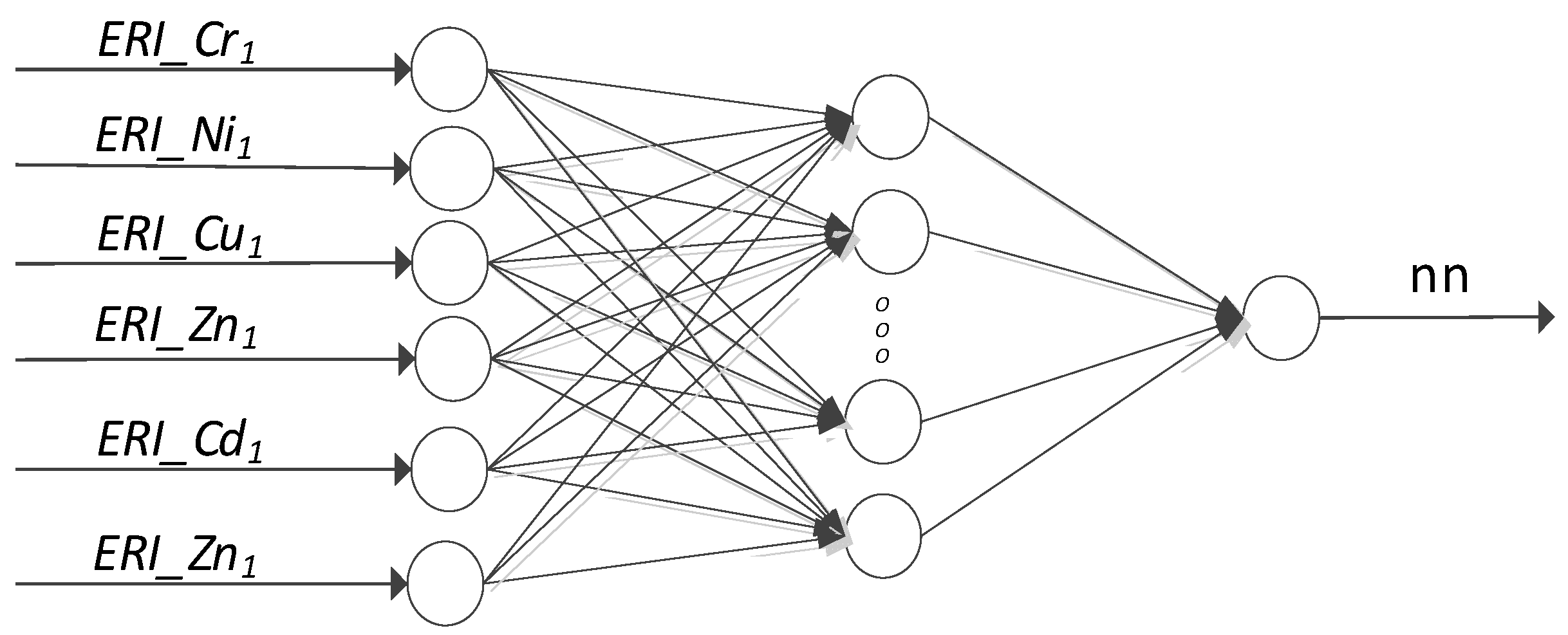
The modeling was performed using Matlab-Neural Network App software. The E R I j values for selected heavy metals at a specified bottom sediment depth level were modeled separately for each metal. A diagram of the neural network is shown in Figure 2. The input layer included the ERI values for each metal in the surface sediment layer (0–5 cm). The output layer corresponded to the predicted ERI value of a given metal in the deeper sediment layer (30 cm).
In the analysis, the primary determinants included the E R I j values of heavy metals such as E R I _ C r 1 ,   E R I _ N i 1 ,   E R I _ C u 1 ,   E R I _ Z n 1 ,   E R I _ C d 1 ,   E R I _ P b 1 within the surface layer (input neurons), and the E R I j value of the modeled metal in the deep layer served as the output neuron. The modeling process employed a feedforward artificial neural network with a single hidden layer network. The quantity of neurons within the hidden layer was established through empirical methods and varied between 2 and 15. The Levenberg–Marquardt training algorithm was selected for its robustness and efficiency in solving nonlinear regression problems. This algorithm combines the advantages of gradient descent and the Gauss–Newton method, making it particularly effective in minimizing the error function in moderately sized datasets. The hidden layer employed a sigmoid activation function to allow for the modeling of nonlinear relationships between input and output variables, while the output layer used a linear activation function (purelin), appropriate for continuous output variables such as ERI. Owing to the limited input data available, the utilization of a separate test set was deemed unnecessary, leading to the partitioning of the complete data set into the following two distinct subsets: training and validation, following an 80:20 split. Identical training and validation datasets were employed for both the MLR and ANN methods. To mitigate overfitting and ensure generalization, early stopping based on validation performance was implemented during training.

2.4. Model Quality Indicators

In order to assess the efficacy of the regression models, the coefficient of determination (R2) was used, which allows for evaluating what portion of the overall variability of the dependent variable is explained by the model, as follows:
R 2 = n = 1 n y ^ i y i 2 n = 1 n y i y i 2 ,
where:
y i —calculated value of E R I j d for the modeled metal at a deeper layer,
y i —arithmetic mean of the values of E R I j (dependent variables of the sample),
y ^ i —value of E R I j for the modeled metal at a deeper layer obtained from the model [32].
To examine the significance of the R 2 value, the F-statistic was used, as follows:
F = R 2 k 1 R 2 n p 1
where:
R 2 coefficient of determination,
k —number of independent variables in the model,
n —total of observations (samples),
p —number of regression model parameters (including the constant).
The t-Student test was employed to ascertain the statistical significance of each individual model parameter, thereby demonstrating a substantial impact of the independent variable on the dependent variable, as follows:
t = β j S E j
where:
β j —vector of the regression model coefficient for index j,
S E j —standard error of the regression coefficient vector [33].
To evaluate the effectiveness of the regression and ANN models, several standard error metrics were used. These included mean squared error (MSE), mean absolute error (MAE), mean absolute percentage error (MAPE), root mean square error (RMSE), regression correlation coefficient (R), and coefficient of determination (R2). The formulas and descriptions are presented as follows:
Mean Squared Error (MSE)
M S E = 1 n n = 1 n y ^ i y i 2
MSE measures the average squared difference between actual ( y i ) and predicted ( y ^ i ) values. It penalizes larger errors more than smaller ones.
Mean Absolute Error (MAE)
M A E = = 1 N i = 1 N y i y ^ i
MAE is the average of the absolute errors. It is less sensitive to outliers than MSE and indicates the average magnitude of the errors in a set of predictions.
Mean Absolute Percentage Error (MAPE)
M A P E = 1 n i = 1 n y i y ^ i y i
MAPE expresses prediction accuracy as a percentage. It is scale-independent and provides an intuitive interpretability, though it is undefined when y i = 0 .
Root Mean Square Error (RMSE)
R M S E = i = 1 n y i y ^ i 2 n
RMSE is the square root of the MSE. It retains the unit of the original output variable and highlights large deviations more than MAE.
Regression Correlation Coefficient (R)
R y , y * = c o v y , y * σ y σ y * , R ϵ < 0,1 >
where:
σ y —standard deviation of calculated value of E R I j   for the modeled metal in the deeper layer,
σ y * —standard deviation of predicted value of E R I j for the modeled metal in the deeper layer.
R represents the proportion of variance in the dependent variable that is predictable from the independent variables. Values closer to 1 indicate a better fit [34,35,36,37].
Together, these indicators provide a robust and multifaceted framework for model evaluation, particularly when analyzing various ANN models and aiming to select the best-performing model. This comprehensive suite of metrics allows for a detailed comparison across different models, ensuring that the chosen model not only fits the current data well, but also reliably predicts E R I j   values under varying conditions.

2.5. Statistical Analysis of Prediction Results

In order to evaluate the statistical significance of the differences between the predictive performances of the artificial neural network and multiple linear regression models, a comprehensive residual analysis was conducted. The analysis aimed to compare the prediction errors for each model with respect to individual heavy metals (Cr, Ni, Cu, Zn, Cd, and Pb) in the deeper sediment layer.
Prior to conducting hypothesis tests, assumptions regarding the distribution of residuals were examined. The normality of residuals for each model was assessed using the Shapiro–Wilk test, while the homogeneity of variances was evaluated using the Brown–Forsythe test. Depending on the fulfillment of these assumptions, appropriate statistical procedures were selected. In cases where both the normality and homogeneity of variance assumptions were met, the standard Student’s t-test for independent samples was applied. If normality was preserved but variance homogeneity was violated, the Cochran–Cox test was used to account for heteroscedasticity. In situations where the residuals did not follow a normal distribution, the Mann–Whitney U test, as a non-parametric alternative, was employed to confirm the robustness of the obtained results.
All tests were conducted at a significance level of α = 0.05. Statistically significant p-values (below the threshold) were interpreted as evidence of a meaningful difference in the predictive accuracy between the ANN and MLR models. The specific results of the applied tests, including the corresponding p-values and test statistics, are presented and discussed in the results section.

3. Results

3.1. Multiple Linear Regression Models

Table 2 shows the results of MLR for the ecological risk index E R I j   values of the chosen heavy metals (Cr, Ni, Cu, Zn, Cd, and Pb) at various bottom sediment depths in Zemborzyce Lake, based on the E R I j   values in the surface layer. The linear regression coefficients indicate how significant the impacts of variables are on the regression model outcomes. The impact of a variable on the model is determined by its β coefficient, even if it is statistically significant. The regression coefficients for significant variables in each model are presented in bold.
The created regression models allow for determining the relationships between metals at different levels of bottom sediments. In each model, E R I j   for a heavy metal shows the influence of the E R I j   levels of other metals. The ecological risk levels for one metal can be partially predicted based on the levels of other heavy metals. This prediction is possible due to the interdependence of heavy metal concentrations in the environment. In the E R I _ C r 2 model, positive influences of E R I _ C r 1 and E R I _ C d 1   and a negative influence of E R I _ P b 1   were noted. The β 1 values for all models showed that an increase in the E R I j of the examined metal had a strong almost linear impact on the E R I j   values of that metal in deeper layers. For the E R I _ N i 2 variable, a low negative influence of E R I _ P b 1 and positive influences of E R I _ C r 1   and E R I _ C d 1 were recorded, along with a significant positive influence of E R I _ N i 1 . For E R I _ C u 2 , a slight positive impact was observed from E R I _ N i 1 and a high E R I _ C u 1 . In the E R I _ Z n 2 model, a significant positive influence of E R I _ Z n 1 and the significance of the intercept were noted, which may mean that there is a certain baseline ecological risk index for zinc that is not influenced by the E R I values of other heavy metals. In turn, E R I _ C d 2 showed a moderate negative influence of E R I _ N i 1 and a positive E R I _ C r 1 ,   E R I _ Z n 1 , and E R I _ C d 1 . The last variable, E R I _ P b 2 , indicated a slight negative impact of E R I _ C u 1 and a positive influence of E R I _ C r 1   E R I _ N i 1 _1, and a high E R I _ P b 1 .
To determine the statistically significant variables in the models presented in Table 3, a t-Student test was conducted with a significance level of α = 0.05. The detailed results of the t-Student tests can be found in Table 3.
T. The t-Student test indicated that the variables E R I _ C r 1 and E R I _ P b 1 were statistically significant at the 0.001 and 0.05 levels, respectively, while E R I _ C d 1   demonstrated significance at the 0.05 level. These findings suggest that all three variables exert a statistically significant influence on E R I _ C r 2 . The analysis of the results for the E R I _ N i 2 model indicated the statistical significance of the impact of the E R I _ C r 1 , E R I _ N i 1 , E R I _ C d 1 , and E R I _ P b 1   variables, as confirmed by the p-values of the t-Student test for each of them. The statistically significant independent variables in the E R I _ C u 2 model were E R I _ N i 1 and E R I _ C u 1 . Other variables had a p-value for the t-Student test greater than 0.05. The variable with a significant impact on the E R I _ Z n 2   dependent variable was E R I _ Z n 1 . Other independent variables were not statistically significant. In the E R I _ C d 2 model, the independent variables with an impact on the dependent variable were E R I _ C r 1 ,   E R I _ N i 1 , E R I _ Z n 1 , and E R I _ C d 1 . The E R I _ C r 1 ,   E R I _ N i 1   , and E R I _ P b 1   variables were statistically significant in the E R I _ P b 2 model, which is confirmed by low p-values. The statistical significance of variables in the models varied. The t-Student test identified which variables were significant for the model. For the models, high t-Student statistic values and low Pr(>|t|) values indicate strong significant relationships between variables.
Table 4 presents key indicators, including individual data set R 2 values, residual ranges, and F-statistic values, for all models predicting the ecological risk index E R I .
Coefficient of determination R2 values serve as a measure of how well a model fits data. All models for the whole dataset (all data) had a very high R2 > 0.98, indicating a very good fit of these models. The models for E R I _ C r 2 ,   E R I _ N i 2 ,   E R I _ C u 2 showed a slightly wider range of residuals compared to the other models, which may indicate greater variability in the data. High F-statistic values for each model (ranging from 402.1 to 17,070) indicate the overall significance of the models. In the E R I Z n 2 model, only one independent variable, E R I _ Z n 1 , was found to be significant, hence, it had the lowest F-statistic value (402.1).
In order to assess the collinearity between the independent variables used to model the environmental risk index (ERI), variance inflation factor (VIF) values were calculated. Table 5 below shows the VIF values for each heavy element (Cr, Ni, Cu, Zn, Cd, and Pb) considered relative to the other variables in the model.
The high values of the VIF coefficients, especially for the last two variables Cd and Pb, testify to the collinearity of the predictors in the model. With this in mind, an analysis of the adjusted R2 coefficient was carried out, taking into account only the statistically significant variables in the model, as shown in Table 3. In addition, the errors of estimation in the least squares method (standard errors) were also analyzed. In the case of a significant deterioration in the redundancy per model, these errors should be much higher than the values of the estimated coefficients and the adjusted R2 should be significantly different from R2. No such effect was observed for the models shown in Table 4. The values of the estimation errors ranged from 1 to 80 percent in individual cases.
When using models for prediction, irrelevant variables are usually not removed from the analysis. It is worth noting that the performance of the prediction models was comparable to that of the network, despite the detected redundancy, so it did not affect the quality of the models.
The models developed demonstrated the ability to predict the ERI of a metal in a deeper layer from the ERIs of other metals in the surface layer. High R2 and F values indicate a strong dependence between metal concentrations and ERI indicators.
The regression method has been used in studies of bottom sediments. Petrosyan et al. (2019) utilized the linear regression approach in order to ascertain the baseline levels of metals present in bottom sediments. The utilization of a linear regression model, along with a comparative element, has been deemed suitable for the assessment of baseline metal concentrations in bottom sediments across various river ecosystems [38]. Ismukhanova et al. (2022) utilized linear regression models for the evaluation of metal contamination within the water–bottom sediment system. The regression analysis model was employed to investigate the associations among metal levels across various soil strata [39]. Deschenes et al. (2013) established a correlation between the concentrations of metals in soils at surface and subsurface levels, except for arsenic, which showed no spatial autocorrelation [40].
The presented studies suggest using MLR analysis to evaluate the correlations between metals in bottom sediment layers. E R I _ C r 1 ,     E R I _ N i 1 ,     E R I _ C u 1 ,     E R I _ P b 1   values were significant variables in the created multiple linear regression models, demonstrating the significant influence they have on sediment layers located at greater depths.

3.2. Artificial Neural Network

The results obtained from the modeling of ecological risk index values related to specific heavy metals j { C r 2 ,   N i 2 ,   C u 2 ,   Z n 2 ,   C d 2 ,   P b 2 } at a specified bottom sediment depth level in Zemborzyce Lake on the basis of the E R I j   values in the surface layer are presented below. For each modeled metal E R I j   value for selected heavy metals, the best network was selected based on MSE, MAE, MAPE, RMSE, R, and R2 indices each.
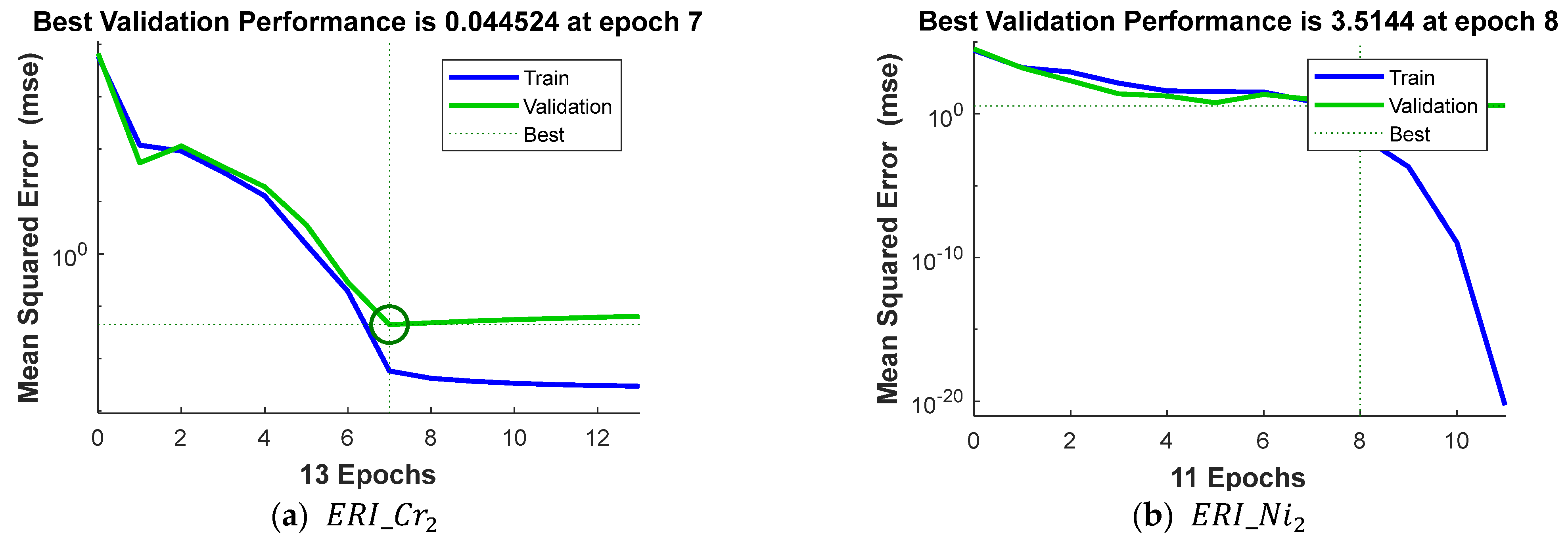
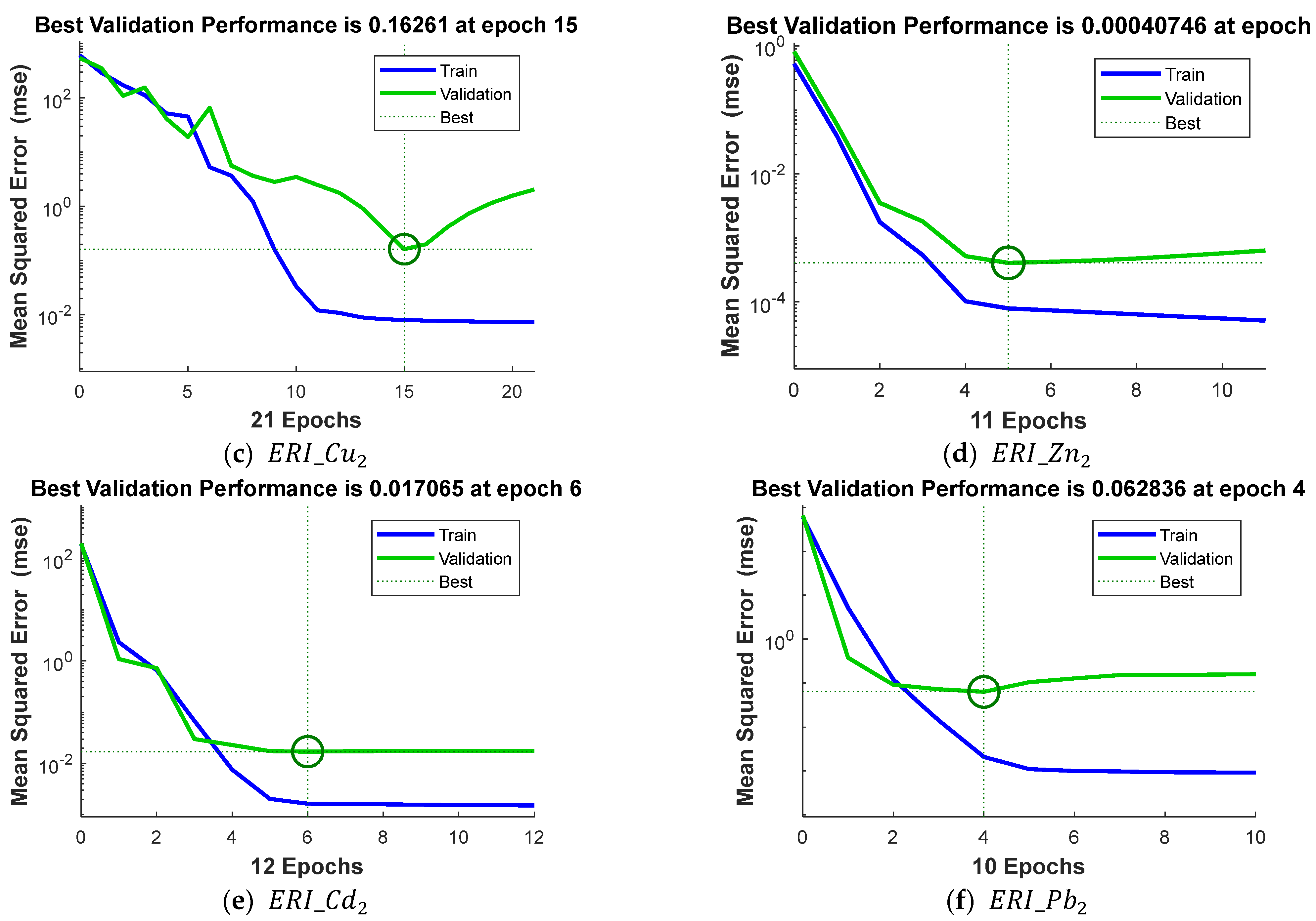
Table 6 shows the results of the training process for each network. The results suggest that creating E R I j   models for selected metals requires different settings and approaches in modeling using neural networks, although the overall network architectures were similar. The number of neurons in the hidden layer is a critical factor in determining the complexity of a network and its ability to map dependencies in data. In the analyzed models, this number ranged from seven to nine neurons. The modeling results for most E R I j   values of heavy metals were best when using networks with eight neurons in the hidden layer, with the exception being the E R I j   values for E R I _ N i 2 , for which the number of neurons in the hidden layer was nine, and E R I _ C u 2 , for which the number of neurons in the hidden layer was 7. The number of epochs—defined as complete passes of the training data through the network—reflects the length of the training process. These values ranged from 10 to 21, suggesting a rapid convergence of the optimization process. The model for E R I _ C u 2 required the most epochs (21), which may indicate a greater complexity or difficulty in modeling this variable. The fewest epochs (10) were needed for E R I _ P b 2 , indicating that it was easier to model. The quality of a model is indicated by its performance, i.e., the training error, which is defined as the discrepancy between the predicted and actual values. A lower value for this indicator suggests a better fit for the model. The lowest error was achieved by the E R I _ N i 2 model, indicating an almost perfect match to the training data. The E R I Z n 2 and E R I _ C d 2 models also demonstrated low error rates, while slightly higher values were observed for the E R I _ C r 2 , E R I _ P b 2 , and E R I _ C u 2 , models, though these were still within acceptable limits. The term ‘gradient’ is used to denote the value of the derivative of the error function in the final training step. When the gradient is minimal, it can be deduced that the model has attained a point near the minimum of the error function. The lowest gradient was, once again, observed in E R I _ N i 2 , indicating that the training process concluded in a state of proximity to the optimum. Conversely, higher gradient values, as observed in E R I _ C r 2 , may signify the potential for further enhancement of the model or the challenge of attaining a stable minimum. The final model indicator that was examined was the best validation error, and the number of epochs in which it was reached. This index is used to determine a model’s ability to generalize. The optimal validation results were obtained for E R I Z n 2 (0.0004 in the fifth epoch), E R I _ C d 2 (0.017 in the sixth epoch), and E R I _ P b 2 (0.0628 in the fourth epoch), demonstrating their excellent capacity to predict new data. The E R I _ C r 2 model achieved a value of 0.0445 in the seventh epoch, which also attained a satisfactory level. The validation error was at its highest for E R I _ N i 2 (3.5144 in the eighth epoch), which may indicate issues with the quality or representativeness of the input data for this metal.
As demonstrated in Figure 3a–c, the training of a neural network model is depicted as a function of the number of epochs, that is, successive complete passes through the entire training set. The vertical axis of these graphs represents the mean squared error (MSE) value on a logarithmic scale, which measures the difference between the model’s predictions and the actual values. It can, thus, be concluded that the lower the MSE value, the better the fit of the model.
Figure 3a–c further illustrate the MSE error on the training (blue line) and validation (green line) sets, along with the optimal validation value of the MSE error attained during epochs (best line). The graphs indicate the points at which the model achieved the lowest error on the validation set and were considered as optimal for the model.
Table 7 presents the results of the network quality indicators of the best networks for all analyzed heavy metals. As illustrated in Figure 4a–f, a comparison is made between the values predicted by the model and real-world observations for the following three data ranges: training, validation, and full dataset (All). Each graph contains data points, a linear regression fit line (a solid-colored line), and a Y = T perfect fit line (dashed line). The latter represents the case of perfect prediction. In all cases, a high degree of agreement was observed between the predicted and actual values. This was confirmed by the regression lines, which exhibited slopes close to unity and minimal deviations from the axes. The high quality of the fit serves as a confirmation of the effectiveness of the artificial neural network model that was utilized.
Low mean squared error values, such as those for E R I _ Z n 2 (MSE = 1.4016 × 10⁻⁴), indicate a better accuracy of the model, while higher values (like for E R I _ N i 2 , MSE = 0.6766) suggest larger errors (Table 6). Similar to MSE, lower values of MAE better determine the quality of the model. For E R I _ C u 2 (MAE = 0.178) and E R I _ N i 2 (MAE = 0.4131), the mean absolute error was relatively high, suggesting larger individual errors in the model.
The model that demonstrated the optimal fit and highest level of stability was the model for the E R I _ Z n 2 index, which was characterized by an extremely low learning error (MSE = 0.0001).
The E R I _ C r 2 and E R I _ C u 2 models exhibited marginally diminished error values in comparison to the E R I _ Z n 2 model. This phenomenon may be attributed to the enhanced variability of the input data, the diminished correlation with the output data, and the potential influence of the geochemical characteristics of the sediments that were not completely encompassed by the model.
The E R I _ N i 2 model demonstrated the highest MSE and MAE error values among all the models analyzed, indicating its suboptimal generalization capability. This may have been due to the significant variations in concentrations, as evidenced by the high standard deviation values for nickel (Ni: 20.84 and 20.15).
In order to enhance the precision of models for less accurate metals, it is possible to construct models that incorporate additional physicochemical parameters, such as pH, granulometric fractions, and organic matter content.
It is evident from the analysis of the models that the MAPE index values were relatively high, with the greatest levels being observed in the models concerning zinc ( E R I _ Z n 2 13.10%) and nickel ( E R I _ N i 2 ,—8.44%). Nevertheless, the elevated MAPE value may be attributable to the inherent specificity of the index. In the event that any metal concentration approaches zero, a substantial percentage error is consequently engendered. As demonstrated in Table 7, the maximum attainable model error percentage values were observed in the E R I _ Z n 2 model, due to the zinc content of the tested sediments attaining the lowest recorded zinc concentration of 0.0204. The variability of sediment composition directly influenced changes in the network quality indicators.
Correlation coefficient values close to one between the predicted and actual values indicate a strong correlation. In the created models for the output variable, E R I _ C r 2 , E R I _ N i 2 , E R I _ C u 2 , E R I _ Z n 2 , E R I _ C d 2 , and E R I _ P b 2 , values very close to 1 R were obtained, indicating a good accuracy of the models.
In this paper, based on the ecological risk index of the surface layer, artificial neural networks were used to predict the ecological risk index values of metals in deeper layers of bottom sediments. The obtained networks had an acceptable error rate, as concluded from the regression value R, MSE, MAE, MAPE, and RMSE. Thus, they can be used as reliable predictors of the E R I j of heavy metals.

3.3. Comparison of MLR and ANN Models

Comparing the results of modeling the ecological risk index values of selected heavy metals ( E R I _ C r 2 , E R I _ N i 2 , E R I _ C u 2 , E R I _ Z n 2 , E R I _ C d 2 , and E R I _ P b 2 )   using the MLR and ANN methods and evaluating the coefficients of determination R2 of the developed models are shown in Table 8. The comparison selected R2 and MSE as standard indicators to interpret both the MLR and ANN models. This effectively predicted the ecological risk index values of the selected heavy metals.
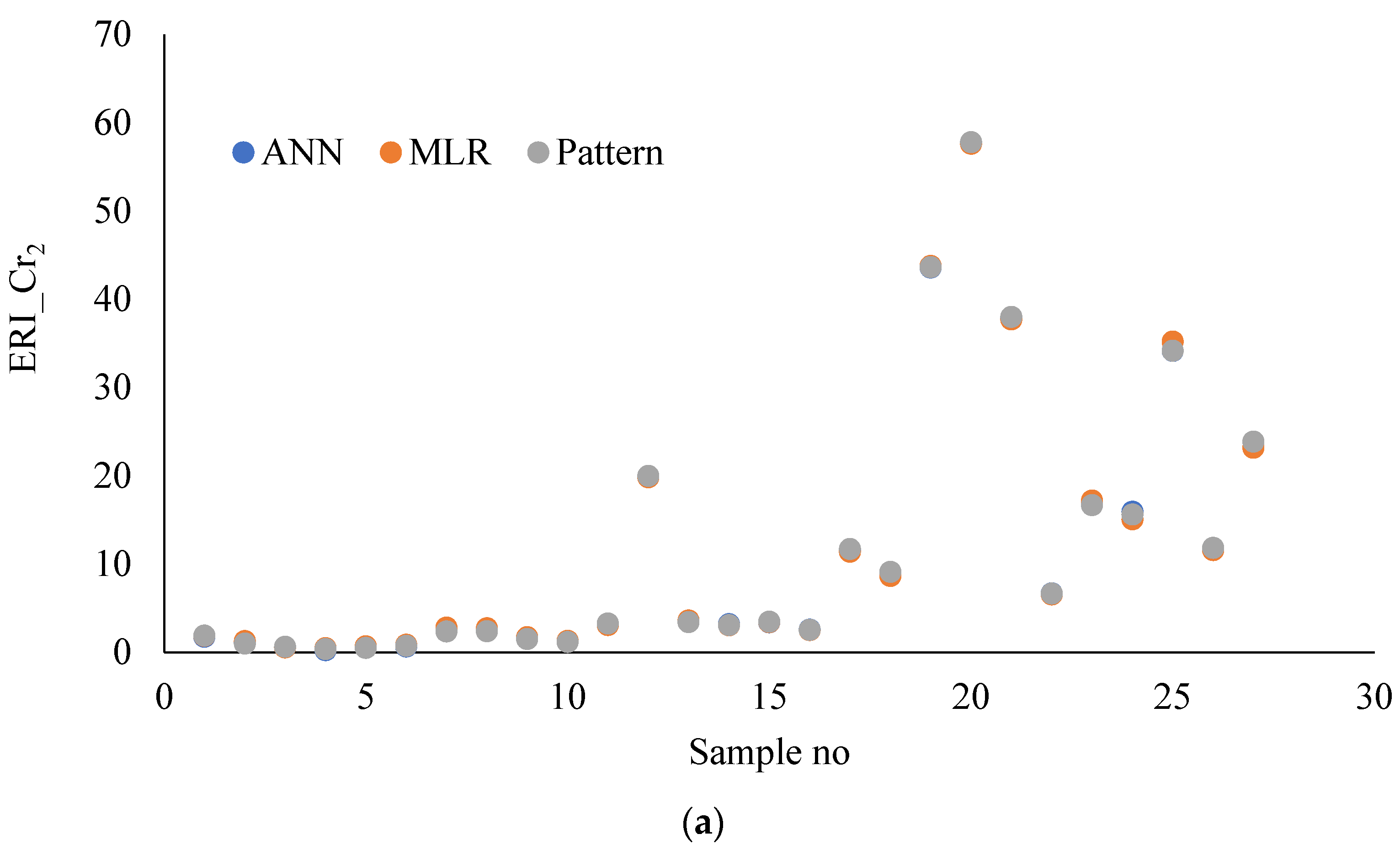
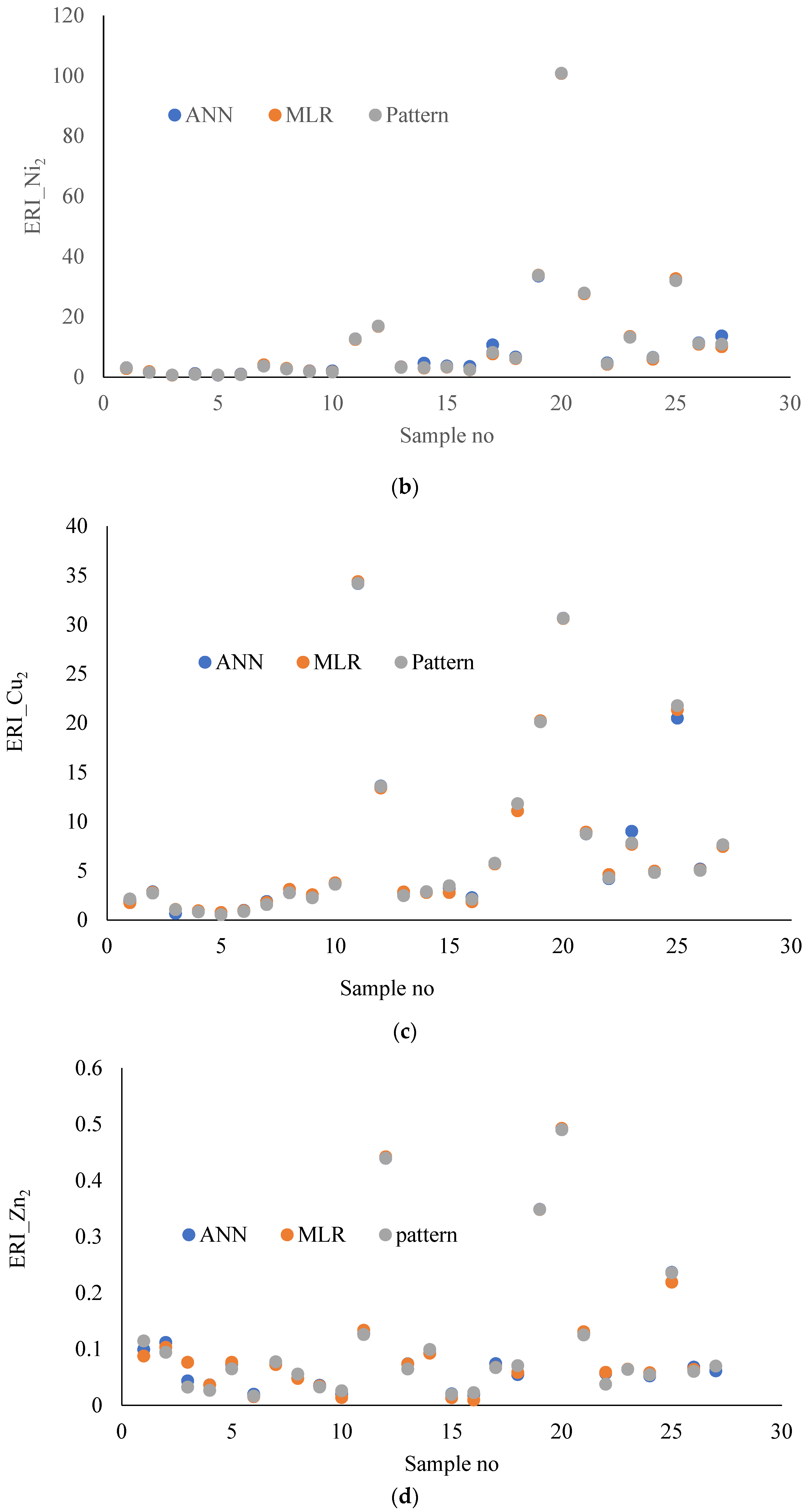
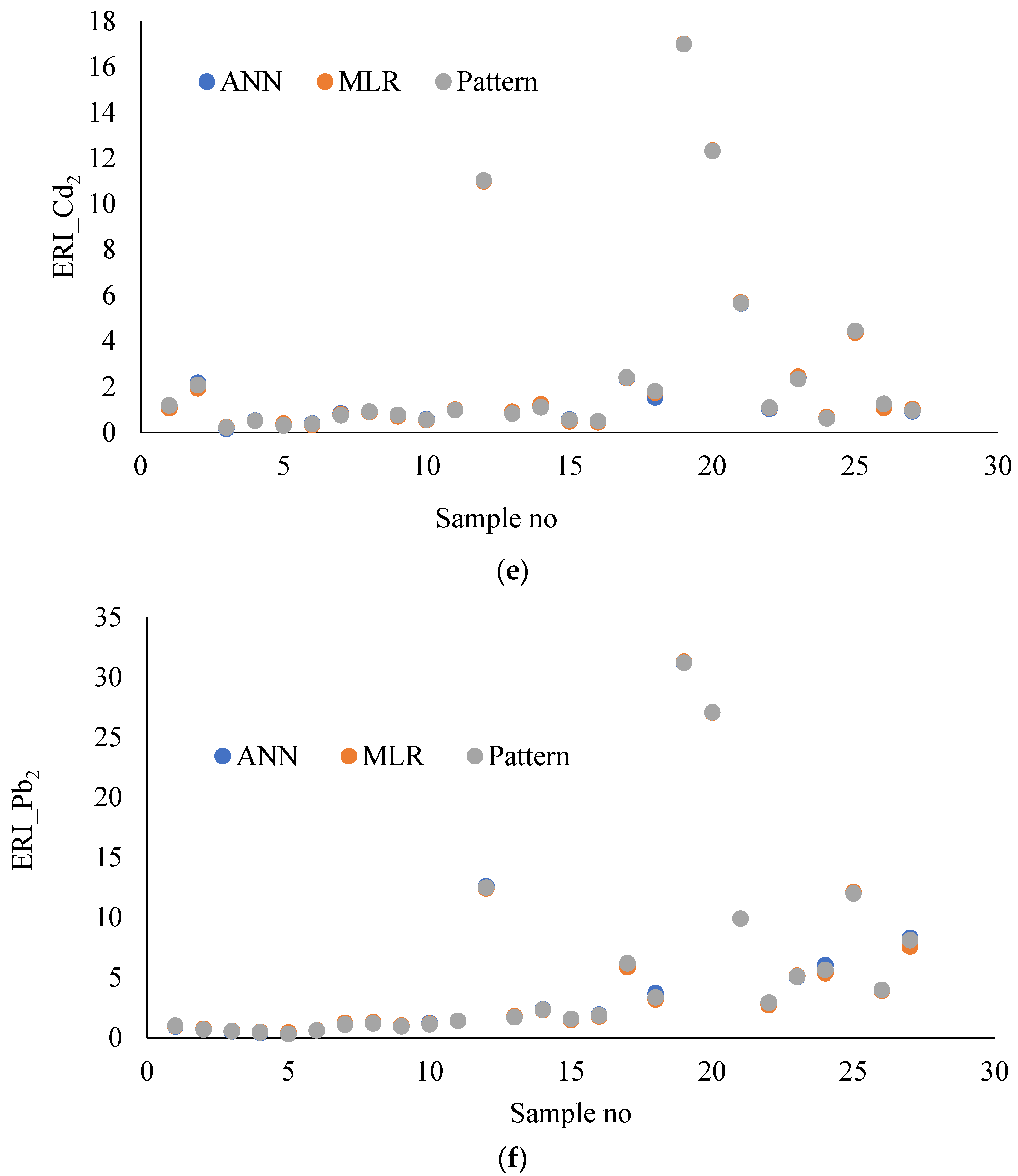
The ANN and MLR models generally showed high coefficients of determination for all metals, indicating a strong predictive power. Due to the complexity of selecting the network architecture and its parameters, such as the number of epochs for each case, choosing the MLR method may prove to be a more efficient and simpler solution. A comparison of the calculated values of E R I j   for the modeled metals E R I _ C r 2 ,     E R I _ N i 2 ,     E R I _ C u 2 ,     E R I _ C d 2 ,   E R I _ Z n 2 ,     E R I _ P b 2 in the deeper layer and the predicted values of E R I j   for the modeled metals in the deeper layer are shown in Figure 5.
In addition to standard performance indicators such as R2 and RMSE, a statistical comparison of the prediction errors obtained from the ANN and MLR models was conducted in order to assess the significance of differences in the predictive accuracy for individual metals (Cr, Ni, Cu, Zn, Cd, and Pb).
The results of the statistical comparison of the prediction errors between the ANN and MLR models are presented in Table 9. The analysis demonstrated that, in most cases, the observed differences in predictive accuracy between the models were not statistically significant. However, selected elements, particularly Ni and to a lesser extent Pb, revealed notable differences in model performance.
It is worth noting that the normality tests conducted for the residuals of the MLR models generally suggested a normal distribution. In the case of Cu, Zn, and Pb, the p-values were close to the significance threshold, and depending on the adopted level of significance, the assumption may or may not be considered as fulfilled. However, the differences were not substantial, and the tests performed were expected to retain sufficient statistical power. Nevertheless, to verify the robustness of the results, the Mann–Whitney U test was additionally employed to assess whether the observed differences would also be detectable using a more conservative non-parametric approach.
Particular attention was paid to the results obtained for Ni and Pb, for which statistically significant differences between the residuals of the two models were observed. In the case of Ni, the assumptions of the Student’s t-test were not fully met due to the lack of normality in the distribution of the ANN model residuals. Nevertheless, the t-test yielded a statistically significant result (p = 0.006), and this finding was independently confirmed by the non-parametric Mann–Whitney test (p = 0.002), which strengthens the credibility of the conclusion, regardless of the violation of parametric assumptions.
A similar situation was observed for Pb, where the t-test indicated a significant difference (p = 0.018), despite the non-normal distribution of ANN residuals. However, in this case, the Mann–Whitney test (p = 0.167) did not confirm this difference, suggesting that the conclusion should be treated with caution and interpreted as inconclusive.
For Cr, the assumption of normality was satisfied, but due to significant variance heterogeneity, the Cochran–Cox test was applied. The result of this test (p = 0.914) did not indicate any statistically significant difference between the models. For the remaining elements (Cu, Zn, and Cd), both parametric and non-parametric tests confirmed the lack of statistically significant differences between the ANN and MLR models.
These findings are consistent with previously reported error metrics such as RMSE and MSE. While the ANN models generally exhibited slightly lower prediction errors, the differences were statistically meaningful only in the case of Ni, and marginally so for Pb. In addition to highlighting the need to use inferential statistics alongside descriptive measures, these findings also underscore the importance of considering broader methodological issues—such as model structure, interpretability, and application context—when choosing prediction tools for environmental analysis.
The predictive accuracy of artificial neural network (ANN) models is often higher than that of classical statistical methods, such as multiple linear regression, due to their nonlinear structure and ability to learn data dependencies independently. ANNs enable the mapping of both linear and nonlinear relationships without necessitating knowledge of the mechanisms governing the modeled process, and they also cope well with a large number of input variables [41].
However, despite its effectiveness, an artificial neural network is regarded as a so-called “black box”—that is, the structure of the model and the way in which decisions are made are difficult to interpret directly [42]. Unlike linear models, an artificial neural network does not provide simple, transparent coefficients that can be directly attributed to specific input variables. This characteristic poses a substantial obstacle for users or stakeholders who value the transparency and explainability of results.
The MLR model is a more transparent and intuitive method for data analysis, as it allows for the direct interpretation of the effects of independent variables on the dependent variable. However, the model is subject to certain limitations, including the assumption of linearity and the lack of consideration of sensitivity to collinearity among independent variables. The effectiveness of the MLR model, as emphasized in the literature, is contingent on the specifics of the application and the nature of the data [43].
There are many studies in the scientific literature that have been conducted to compare the ANN and MLR models in various application domains [44,45,46,47], which confirms that the selection of the model should depend not only on the anticipated accuracy, but also on the necessity to comprehend the structure of dependencies and the application context. In scenarios where the clarity and interpretability of results are paramount (e.g., in environmental studies or stakeholder reporting), the MLR model may be a more suitable option, despite its slightly lower accuracy. However, in contexts where maximum prediction efficiency is of the essence, the utilization of ANN models is strongly advised.

4. Conclusions

The study investigated the feasibility of using machine learning methods to predict the ecological risk index values of metals in the deeper layer of bottom sediments based on the E R I values of metals in the surface layer. For this purpose, 27 bottom sediment samples were collected from the surface layer (0–5 cm) and deeper layer (30 cm) of Zemborzyce Lake (Lublin, Poland) and then analyzed to determine the concentrations of the following metals: Cd, Cr, Cu, Ni, Pb, and Zn. These concentrations were used to calculate the ecological risk index values of the metals.
The MLR models showed that the E R I _ C r 1 ,     E R I _ N i 1 ,     E R I _ C u 1 ,     E R I _ P b 1 variables were statistically significant, indicating their influence on ERI indicators in deeper sediment layers. All MLR models showed an R greater than 0.99, indicating a good fit. The ANN models were characterized by low errors (MSE, MAE, and RMSE) and high R2 values, close to one, for all the output variables, indicating their high accuracy and ability to predict ERI values for different metals (Cr, Ni, Cu, Zn, Cd, and Pb). The largest error (highest MAPE value) occurred for the   E R I _ Z n 2 variable, which may indicate a greater difficulty in predicting this particular variable compared to other metals.
Both the artificial neural network (ANN) and multiple linear regression (MLR) models demonstrated high coefficients of determination for several heavy metals, indicating strong predictive capabilities in modeling the ecological risk index in bottom sediments. The effectiveness of these approaches supports the use of data analytics for forecasting contamination levels in deeper sediment layers based on surface sediment data.
While ANN models offer a high accuracy, their implementation can be more complex due to the need for optimizing network architecture parameters such as the number of neurons, epochs, and activation functions. In this context, MLR proves to be not only efficient, but also more transparent and easier to implement, which is particularly relevant for practical applications in water and energy resource management.
The results confirm that machine learning methods can serve as effective tools for assessing the ecological risk from heavy metal pollution in water bodies used for energy production. The use of predictive approaches can support better sediment management, contributing to the protection of hydropower infrastructure and the sustainability of energy systems relying on aquatic environments.

Author Contributions

Conceptualization, B.P. and M.K.; methodology, B.P., M.K., J.K., M.C., A.G. and R.G.; software, M.K. and M.C.; validation, B.P., M.K., J.K., M.C. and A.G.; formal analysis, B.P., M.K., J.K., M.C., A.G. and R.G.; investigation, J.K. and A.G.; resources, B.P., M.K., J.K., M.C. and A.G.; data curation, B.P., M.K., J.K., M.C. and A.G.; writing—original draft preparation, B.P., M.K., J.K., M.C. and A.G.; writing—review and editing, B.P., M.K., J.K. and R.G.; visualization, B.P., M.K., J.K., M.C., A.G. and R.G.; supervision, B.P.; project administration, J.K.; funding acquisition, B.P., M.K., J.K. and M.C. All authors have read and agreed to the published version of the manuscript.

Funding

This research was funded by the POLISH MINISTRY OF SCIENCE AND HIGHER EDUCATION, grant numbers: FD-NZ-020/2024, FD-20/IS-6/019, FD-NZ-999/2024 and FD-20/IM-5/088.

Data Availability Statement

Data are contained within the article. Data supporting this study are included within the article.

Conflicts of Interest

The authors declare no conflicts of interest.

References

  1. Li, S.; Xu, Y.J.; Ni, M. Changes in Sediment, Nutrients and Major Ions in the World Largest Reservoir: Effects of Damming and Reservoir Operation. J. Clean. Prod. 2021, 318, 128601. [Google Scholar] [CrossRef]
  2. Akhtar, N.; Syakir Ishak, M.I.; Bhawani, S.A.; Umar, K. Various natural and anthropogenic factors responsible for water quality degradation: A review. Water 2021, 13, 2660. [Google Scholar] [CrossRef]
  3. Chen, X.; Wang, Y.; Sun, T.; Huang, Y.; Chen, Y.; Zhang, M.; Ye, C. Effects of Sediment Dredging on Nutrient Release and Eutrophication in the Gate-Controlled Estuary of Northern Taihu Lake. J. Chem. 2021, 2021, 1–13. [Google Scholar] [CrossRef]
  4. Dalu, T.; Tshivhase, R.; Cuthbert, R.N.; Murungweni, F.M.; Wasserman, R.J. Metal Distribution and Sediment Quality Variation Declared Wetland. Water 2020, 12, 2779. [Google Scholar] [CrossRef]
  5. Xu, Q.; Zhou, K.; Wu, B. Dam Construction Reshapes Heavy Metal Pollution in Soil/Sediment in the Three Gorges Reservoir, China, from 2008 to 2020. Front. Environ. Sci. 2023, 11, 1269138. [Google Scholar] [CrossRef]
  6. Sojka, M.; Jaskuła, J.; Barabach, J.; Ptak, M.; Zhu, S. Heavy metals in lake surface sediments in protected areas in Poland: Concentration, pollution, ecological risk, sources and spatial distribution. Sci. Rep. 2022, 12, 15006. [Google Scholar] [CrossRef]
  7. Hossain, M.A.; Furumai, H.; Nakajima, F.; Aryal, R.K. Heavy metals speciation in sediment accumulated within an infiltration facility and evaluation of metal retention properties of underlying soil. Water Sci. Technol. 2007, 56, 827–834. [Google Scholar] [CrossRef]
  8. Shahbazi, K.; Beheshti, M. Comparison of three methods for measuring heavy metals in calcareous soils of Iran. SN Appl. Sci. 2019, 1, 1541. [Google Scholar] [CrossRef]
  9. Sastre, J.; Sahuquillo, A.; Vidal, M.; Rauret, G. Determination of Cd, Cu, Pb and Zn in environmental samples: Microwave-assisted total digestion versus aqua regia and nitric acid extraction. Anal. Chim. Acta 2002, 462, 59–72. [Google Scholar] [CrossRef]
  10. Zhong, X.L.; Zhou, S.L.; Zhu, Q.; Zhao, Q.G. Fraction distribution and bioavailability of soil heavy metals in the Yangtze River Delta-A case study of Kunshan City in Jiangsu Province, China. J. Hazard. Mater. 2011, 198, 13–21. [Google Scholar] [CrossRef]
  11. Brady, J.P.; Ayoko, G.A.; Martens, W.N.; Goonetilleke, A. Development of a hybrid pollution index for heavy metals in marine and estuarine sediments. Environ. Monit. Assess. 2015, 187, 306. [Google Scholar] [CrossRef]
  12. Bhagat, S.K.; Tung, T.M.; Yaseen, Z.M. Heavy metal contamination prediction using ensemble model: Case study of Bay sedimentation, Australia. J. Hazard. Mater. 2021, 403, 123492. [Google Scholar] [CrossRef] [PubMed]
  13. Aljahdali, M.O.; Alhassan, A.B. Ecological risk assessment of heavy metal contamination in mangrove habitats, using biochemical markers and pollution indices: A case study of Avicennia marina L. in the Rabigh lagoon, Red Sea. Saudi J. Biol. Sci. 2020, 27, 1174–1184. [Google Scholar] [CrossRef] [PubMed]
  14. Sidoruk, M. Pollution and Potential Ecological Risk Evaluation of Heavy Metals in the Bottom Sediments: A Case Study of Eutrophic Bukwałd Lake Located in an Agricultural Catchment. Int. J. Environ. Res. Public Health 2023, 20, 2387. [Google Scholar] [CrossRef] [PubMed]
  15. Ramseyer, C.A.; Miller, P.W.; Mote, T.L. Future precipitation variability during the early rainfall season in the El Yunque National Forest. Sci. Total Environ. 2019, 661, 326–336. [Google Scholar] [CrossRef]
  16. Iqbal, M.; Ali Naeem, U.; Ahmad, A.; Rehman, H.-u.; Ghani, U.; Farid, T. Relating groundwater levels with meteorological parameters using ANN technique. Measurement 2020, 166, 108163. [Google Scholar] [CrossRef]
  17. Venkateswarlu, T.; Anmala, J.; Dharwa, M. PCA, CCA, and ANN Modeling of Climate and Land-Use Effects on Stream Water Quality of Karst Watershed in Upper Green River, Kentucky. J. Hydrol. Eng. 2020, 25, 05020008. [Google Scholar] [CrossRef]
  18. Fabregat, A.; Vázquez, L.; Vernet, A. Using Machine Learning to estimate the impact of ports and cruise ship traffic on urban air quality: The case of Barcelona. Environ. Model. Softw. 2021, 139, 104995. [Google Scholar] [CrossRef]
  19. Liu, X.-F.; Zhu, H.-H.; Wu, B.; Li, J.; Liu, T.-X.; Shi, B. Artificial intelligence-based fiber optic sensing for soil moisture measurement with different cover conditions. Measurement 2023, 206, 112312. [Google Scholar] [CrossRef]
  20. Stachurska, B.; Mahdavi-Meymand, A.; Sulisz, W. Machine learning methodology for determination of sediment particle velocities over sandy and rippled bed. Measurement 2022, 197, 111332. [Google Scholar] [CrossRef]
  21. Świetlicka, I.; Sujak, A.; Muszyński, S.; Świetlicki, M. The application of artificial neural networks to the problem of reservoir classification and land use determination on the basis of water sediment composition. Ecol. Indic. 2017, 72, 759–765. [Google Scholar] [CrossRef]
  22. Mohammed, H.; Michel Tornyeviadzi, H.; Seidu, R. Emulating process-based water quality modelling in water source reservoirs using machine learning. J. Hydrol. 2022, 609, 127675. [Google Scholar] [CrossRef]
  23. García Nieto, P.J.; Alonso Fernández, J.R.; De Cos Juez, F.J.; Sánchez Lasheras, F.; Díaz Muñiz, C. Hybrid modelling based on support vector regression with genetic algorithms in forecasting the cyanotoxins presence in the Trasona reservoir (Northern Spain). Environ. Res. 2013, 122, 1–10. [Google Scholar] [CrossRef]
  24. Bhagat, S.K.; Tung, T.M.; Yaseen, Z.M. Development of artificial intelligence for modeling wastewater heavy metal removal: State of the art, application assessment and possible future research. J. Clean. Prod. 2020, 250, 119473. [Google Scholar] [CrossRef]
  25. El Chaal, R.; Aboutafail, M.O. Comparing Artificial Neural Networks with Multiple Linear Regression for Forecasting Heavy Metal Content. Acadlore Trans. Geosci. 2022, 1, 2–11. [Google Scholar] [CrossRef]
  26. Manssouri, I.; El Hmaidi, A.; Manssouri, T.E.; Moumni, B. El Prediction levels of heavy metals (Zn, Cu and Mn) in current Holocene deposits of the eastern part of the Mediterranean Moroccan margin (Alboran Sea). IOSR J. Comput. Eng. 2014, 16, 117–123. [Google Scholar] [CrossRef]
  27. Abdallaoui, A.; El Badaoui, H. Comparative study of two stochastic models using the physicochemical characteristics of river sediment to predict the concentration of toxic metals. J. Mater. Environ. Sci. 2015, 6, 445–454. [Google Scholar]
  28. Venkatramanan, S.; Chung, S.Y.; Selvam, S.; Son, J.H.; Kim, Y.J. Interrelationship between geochemical elements of sediment and groundwater at Samrak Park Delta of Nakdong River Basin in Korea: Multivariate statistical analyses and artificial neural network approaches. Environ. Earth Sci. 2017, 76, 456. [Google Scholar] [CrossRef]
  29. ISO 14869-1:2000; Soil Quality—Dissolution for the Determination of Total Element Content—Part 1: Dissolution with Hydrofluoric and Perchloric Acids. International Organization for Standardization: Geneva, Switzerland, 2000.
  30. Hattab, N.; Hambli, R.; Motelica-Heino, M.; Bourrat, X.; Mench, M. Application of neural network model for the prediction of chromium concentration in phytoremediated contaminated soils. J. Geochem. Explor. 2013, 128, 25–34. [Google Scholar] [CrossRef]
  31. Mgbenu, C.N.; Egbueri, J.C. The hydrogeochemical signatures, quality indices and health risk assessment of water resources in Umunya district, southeast Nigeria. Appl. Water Sci. 2019, 9, 22. [Google Scholar] [CrossRef]
  32. Chicco, D.; Warrens, M.J.; Jurman, G. The coefficient of determination R-squared is more informative than SMAPE, MAE, MAPE, MSE and RMSE in regression analysis evaluation. PeerJ Comput. Sci. 2021, 7, e623. [Google Scholar] [CrossRef] [PubMed]
  33. Plonsky, L.; Ghanbar, H. Multiple Regression in L2 Research: A Methodological Synthesis and Guide to Interpreting R2 Values. Mod. Lang. J. 2018, 102, 713–731. [Google Scholar] [CrossRef]
  34. Hodson, T.O. Root-mean-square error (RMSE) or mean absolute error (MAE): When to use them or not. Geosci. Model Dev. 2022, 15, 5481–5487. [Google Scholar] [CrossRef]
  35. Robeson, S.M.; Willmott, C.J. Decomposition of the mean absolute error (MAE) into systematic and unsystematic components. PLoS ONE 2023, 18, e0279774. [Google Scholar] [CrossRef]
  36. Kim, S.; Kim, H. A new metric of absolute percentage error for intermittent demand forecasts. Int. J. Forecast. 2016, 32, 669–679. [Google Scholar] [CrossRef]
  37. Yarar, A. Analytical and artificial neural network models to estimate the discharge coefficient for ogee spillway. E3S Web Conf. 2017, 19, 03028. [Google Scholar] [CrossRef]
  38. Petrosyan, V.; Pirumyan, G.; Perikhanyan, Y. Determination of heavy metal background concentration in bottom sediment and risk assessment of sediment pollution by heavy metals in the Hrazdan River (Armenia). Appl. Water Sci. 2019, 9, 102. [Google Scholar] [CrossRef]
  39. Ismukhanova, L.; Choduraev, T.; Opp, C.; Madibekov, A. Accumulation of Heavy Metals in Bottom Sediment and Their Migration in the Water Ecosystem of Kapshagay Reservoir in Kazakhstan. Appl. Sci. 2022, 12, 1474. [Google Scholar] [CrossRef]
  40. Deschenes, S.; Setton, E.; Demers, P.A.; Keller, P.C. Exploring the Relationship between Surface and Subsurface Soil Concentrations of Heavy Metals using Geographically Weighted Regression. E3S Web Conf. 2013, 1, 35007. [Google Scholar] [CrossRef]
  41. Hosseinzadeh, A.; Najafpoor, A.A.; Jonidi Jafari, A.; Khani Jazani, R.; Baziar, M.; Bargozin, H.; Ghasemy Piranloo, F. Application of response surface methodology and artificial neural network modeling to assess non-thermal plasma efficiency in simultaneous removal of BTEX from waste gases: Effect of operating parameters and prediction performance. Process Saf. Environ. Prot. 2018, 119, 261–270. [Google Scholar] [CrossRef]
  42. Linardatos, P.; Papastefanopoulos, V.; Kotsiantis, S. Explainable AI: A Review of Machine Learning Interpretability Methods. Entropy 2021, 23, 18. [Google Scholar] [CrossRef] [PubMed]
  43. Zhang, Y.; Wang, L.; Li, X.; Chen, Y.; Liu, Z. Analysis of mechanical properties for tea stem using grey relational analysis coupled with multiple linear regression. Sci. Hortic. 2020, 261, 108886. [Google Scholar] [CrossRef]
  44. Cascone, S.; Catania, F.; Gagliano, A.; Sciuto, G. Energy performance and environmental and economic assessment of the platform frame system with compressed straw. Energy Build. 2018, 166, 83–92. [Google Scholar] [CrossRef]
  45. Kim, Y.S.; Ko, S.J.; Lee, S.; Seok, S.; Lee, J.S.; Jeung, G.W.; Chung, H.J. Optimizing anode location in impressed current cathodic protection system to minimize underwater electric field using multiple linear regression analysis and artificial neural network methods. Eng. Anal. Bound. Elem. 2018, 96, 84–93. [Google Scholar] [CrossRef]
  46. Jia, J.; Lee, W.L. The Rising Energy Efficiency of Office Buildings in Hong Kong. Energy Build. 2018, 166, 296–304. [Google Scholar] [CrossRef]
  47. Hosseinzadeh, A.; Baziar, M.; Alidadi, H.; Zhou, J.L.; Altaee, A.; Najafpoor, A.A.; Jafarpour, S. Application of artificial neural network and multiple linear regression in modeling nutrient recovery in vermicompost under different conditions. Bioresour. Technol. 2020, 303, 122926. [Google Scholar] [CrossRef]
Figure 1. Map of the study area (a). Spatial distribution ERJ of Cr (b), Ni (c), Cu (d), Zn (e), Cd (f), and Pb (g), and counts in the bottom sediments of the lake (black dots).
Energies 18 02329 g001
Figure 2. Diagram of the neural network, where nn denotes the E R I value for selected heavy metals, respectively, E R I _ C r 2 ,   E R I _ N i 2 ,   E R I _ C u 2 ,   E R I _ Z n 2 ,   E R I _ C d 2 ,   E R I _ P b 2 on the deeper layer.
Energies 18 02329 g002
Figure 3. Mean Squared Error (MSE) during model training over examined epochs. Best validation performance for best networks for ERI_(-j) value for heavy metals: (a) E R I _ C r 2 ,   ( b) E R I _ N i 2 ,   ( c) E R I _ C u 2 ,   (d) E R I _ Z n 2 , (e) E R I _ C d 2 , and (f) E R I _ P b 2 .
Energies 18 02329 g003aEnergies 18 02329 g003b
Figure 4. Regression plots for training, validation, and all data sets for individual models for: (a) E R I _ C r 2 , (b) E R I _ N i 2 , (c) E R I _ C u 2 , (d) E R I _ Z n 2 , (e) E R I _ C d 2 , and (f) E R I _ P b 2 . The relationship between the expected value (“Target”) and the actual output value of the model (“Output”).
Energies 18 02329 g004
Figure 5. A comparison of calculated and predicted value of ERI_(−j) for the modeled metal on the deeper layer for: (a) E R I _ C r 2 , (b) E R I _ N i 2 ,   (c) E R I _ C u 2 ,   (d) E R I _ Z n 2 , (e) E R I _ C d 2 , and (f) E R I _ P b 2 .
Energies 18 02329 g005aEnergies 18 02329 g005bEnergies 18 02329 g005c
Table 1. Data for statistical analysis.
The Ecological Risk
Index
Min.MaxMeanSD
I Level (0–5 cm)
E R I _ C r 0.364259.331312.090015.7622
E R I _ N i 1 0.8017104.209312.019920.8369
E R I _ C u 1 0.698837.08347.78699.3036
E R I _ Z n 1 0.02040.46500.11089.3036
E R I _ C d 1 0.202017.29992.72494.2499
E R I _ P b 1 0.386233.71335.56818.1280
II level (30 cm)
E R I _ C r 2 0.345957.778011.748015.3052
E R I _ N i 2 0.6522100.811811.621120.1526
E R I _ C u 2 0.543634.19447.61659.0197
E R I _ Z n 2 0.01660.49050.10880.1246
E R I _ C d 2 0.202316.99652.67704.1616
E R I _ P b 2 0.308531.19465.35477.7168
Table 2. Coefficients for explanatory variables in the multiple regression model.
Model β 0 β 1   ( E R I _ C r 1 ) β 2   ( E R I _ N i 1 ) β 3   ( E R I _ C u 1 ) β 4   ( E R I _ Z n 1 ) β 5   ( E R I _ C d 1 ) β 6   ( E R I _ P b 1 )
E R I _ C r 2 0.1281.0200.009−0.013−1.7910.255−0.217
E R I _ N i 2 0.1040.0400.978−0.015−3.4600.359−0.224
E R I _ C u 2 0.0440.0190.0280.9120.8270.010−0.041
E R I _ Z n 2 −0.0110.001−0.0000.0001.0740.000−0.002
E R I _ C d 2 −0.0590.009−0.010−0.0001.1770.965−0.003
E R I _ P b 2 −0.0150.0190.012−0.0090.9180.0370.866
Table 3. t-Student test values for significant model variables.
ModelSignificant Variablet-StudentPr(>|t|) < 0.05
E R I _ C r 2 E R I _ C r 1 55.7430.0000 ***
E R I _ C d 1 2.2150.0427 *
E R I _ P b 1 −3.6490.0024 **
E R I _ N i 2 E R I _ C r 1 2.7750.0142 *
E R I _ N i 1 106.6520.0000 ***
E R I _ C d 1 3.8640.0015 **
E R I _ P b 1 −4.9240.0002 ***
E R I _ C u 2 E R I _ N i 1 2.7810.014 *
E R I _ C u 1 77.6870.0000 ***
E R I _ Z n 2 E R I _ Z n 1 14.9030.0000 ***
E R I _ C d 2 E R I _ C r 1 2.3300.0342 *
E R I _ N i 1 −4.1620.0008 ***
E R I _ Z n 1 2.2390.0407 *
E R I _ C d 1 37.6160.0000 ***
E R I _ P b 2 E R I _ C r 1 3.0990.0073 **
E R I _ N i 1 2.7350.0153 *
E R I _ C u 1 −2.1360.0496 *
E R I _ P b 1 41.4860.0000 ***
E R I _ C r 1 3.0990.0073 **
* Significant codes: ‘***’ 0.001, ‘**’ 0.01, and ‘*’ 0.05.
Table 4. Quality indicators of the models.
R2 (Training Data)R2 (Test Data)R2 (All Data)Adjusted R2MinMaxF-Statistic
E R I _ C r 2 0.99950.99640.99950.9993−1.02770.70685243
E R I _ N i 2 0.99990.98720.99980.9998−0.65340.519117,070
E R I _ C u 2 0.99890.99930.99900.9985−0.38000.72942275
E R I _ Z n 2 0.99380.51940.98860.9914−0.02110.0270402
E R I _ C d 2 0.99980.98330.99970.9997−0.13070.175310,110
E R I _ P b 2 0.99980.98810.99960.9998−0.14240.324514,750
Table 5. Matrix of VIFs for multiple linear regression models with different dependent variables.
E R I _ C r 1 E R I _ N i 1 E R I _ C u 1 E R I _ Z n 1 E R I _ C d 1 E R I _ P b 1
E R I _ C r 2 11.18547.66302.099111.553133.610332.1656
E R I _ N i 2 12.63459.19922.092512.50939.026534.4673
E R I _ C u 2 12.65087.92532.024512.464132.933129.3474
E R I _ Z n 2 11.11197.22482.062111.092028.490228.6835
E R I _ C d 2 12.36399.31312.166712.869241.611734.8320
E R I _ P b 2 14.087711.7922.249215.420955.800342.9049
Table 6. Training results of neural networks for best networks for E R I j values of selected heavy metals analyzed.
Model for Output Variable E R I _ C r 2 E R I _ N i 2 E R I _ C u 2 E R I _ Z n 2 E R I _ C d 2 E R I _ P b 2
Neurons in hidden layer897888
Epoch131121111210
Performance0.0035.24 × 10−210.00735.1 × 10−50.00150.0009
Gradient0.1867.71 × 10−90.07530.00030.0110.009
Best validation performance (at epoch)0.0445
(7)
3.5144
(8)
0.1626
(15)
0.0004
(5)
0.017
(6)
0.0628
(4)
Table 7. Results of network quality indicators for best networks for ERI_(-j) for all heavy metals analyzed.
Model for Output Variable E R I _ C r 2 E R I _ N i 2 E R I _ C u 2 E R I _ Z n 2 E R I _ C d 2 E R I _ P b 2
MSE0.01290.67660.03660.00010.00450.0133
MAE0.08900.41310.17830.00760.04220.0680
MAPE 6.40498.43606.365013.10195.28163.9053
RMSE0.11380.82260.36210.01180.06700.1155
R (all data)0.99990.99930.99980.99550.99980.9999
R20.99990.99830.99950.99530.99970.9999
Table 8. Comparison of the coefficients of determination R2 and MSE for predictive models of the ecological risk index ( E R I j ) values of selected heavy metals ( E R I _ C r 2 , E R I _ N i 2 , E R I _ C u 2 , E R I _ Z n 2 , E R I _ C d 2 , and E R I _ P b 2 ) for MLR and ANN methods.
Model for Output Variable E R I _ C r 2 E R I _ N i 2 E R I _ C u 2 E R I _ Z n 2 E R I _ C d 2 E R I _ P b 2
MLR
MSE0.12000.08940.08160.00020.00520.0238
R20.99950.99980.99900.98860.99970.9996
ANN
MSE0.01290.67660.03660.00010.00450.0133
R20.99990.99830.99950.99530.99970.9999
Table 9. Results of statistical tests comparing prediction errors between ANN and MLR models for individual metals.
E R I _ C r 2 E R I _ N i 2 E R I _ C u 2 E R I _ Z n 2 E R I _ C d 2 E R I _ P b 2
Normality (Shapiro–Wilk)ANN0.07500.0000.0000.5890.0000.000
MLR0.55600.8750.0340.0370.9500.020
Variance equality (Brown–Forsythe)0.00090.2430.5960.1890.2280.160
t-test0.914 *0.0060.8590.8830.9940.018
Mann–Whitney U test-0.0020.6040.9040.8900.167
* Cochran–Cox test used due to unequal variances.
Disclaimer/Publisher’s Note: The statements, opinions and data contained in all publications are solely those of the individual author(s) and contributor(s) and not of MDPI and/or the editor(s). MDPI and/or the editor(s) disclaim responsibility for any injury to people or property resulting from any ideas, methods, instructions or products referred to in the content.