Optimized Feedback Type Flux Weakening Control of Non-Salient Permanent Magnet Synchronous Machines in MTPV Region with Improved Stability

Abstract

This paper introduces an enhanced approach for optimizing the flux-weakening performance of a non-salient permanent magnet synchronous machine (PMSM), by incorporating the maximum torque per voltage (MTPV) region into a conventional voltage magnitude feedback control strategy. The MTPV control strategy is initially optimized for steady-state performance by incorporating the effect of resistance, which plays a crucial role in small power motors. To maintain stability and good dynamics in the flux-weakening region, a current command feedback MTPV controller is utilized, as opposed to a voltage command feedback approach. Additionally, to address stability concerns in the MTPV region, a feedback type proportional-integral (PI) MTPV controller is designed and implemented. The stability in both the over-modulation and various flux-weakening regions is further enhanced using a voltage vector modifier (VVM). Therefore, the proposed feedback-based flux-weakening control enhances system steady-state performance, dynamic response, and stability across both linear and over modulation regions under various flux-weakening conditions, making it suitable for general-purpose applications. The effectiveness of the proposed method is validated through experimental results.

1. Introduction

Permanent magnet synchronous machine (PMSM) is widely used in applications such as electric vehicles, aerospace, and industrial automation due to its high efficiency and high torque/power density [1]. To extend the speed operation range under the physical limit of the machine and inverter, the flux-weakening methods are normally employed [2].

Within the conventional current vector control framework, flux-weakening methods have been developed to optimize current commands under current and voltage constraints [3]. The current commands can be obtained by the feedforward [4,5], voltage feedback [6,7], and hybrid methods [8,9]. While the feedforward method offers excellent transient performance [10], its effectiveness is significantly affected by variations in machine parameters. For the small power machine, the complexity of the optimal d- and q-axis current equations increases significantly when the resistance is considered [11]. In [11], a piecewise linearization method is employed to realize a simplified current trajectory, making it suitable for low-cost applications. Nevertheless, this approach is unable to generate the optimal current trajectory in the flux-weakening region.

By introducing a voltage feedback loop, the voltage feedback method enables automatic flux-weakening control [12]. It can achieve an optimal current trajectory and have robustness against variation of the machine parameters [13]. The implementation of the feedback method is much simpler than the hybrid method which requires both feedback and feedforward paths. Owing to its simplicity, the voltage feedback method has been widely adopted in both low-cost applications and industrial practices [14]. However, the feedback controller requires the proper tuning of control parameters. In [15] and [16], an adaptive control parameter method is employed to enable a stable and extended flux-weakening operation range. However, its application is restricted to the linear modulation region (LMR). While the LMR offers improved dynamics and reduced current harmonics, it comes at the cost of reduced DC-link voltage utilization.

In the flux-weakening and over-modulation regions, a reduction in the voltage control margin may lead to conflicts between the dq-axis current controllers, potentially resulting in oscillations and instability [17]. Reference [17] proposes using a single d-axis current controller, while leaving the q-axis voltage in an open-loop configuration, effectively resolving the conflict between the d- and q-axis current controllers. However, the q-axis voltage reference relies on the machine parameters, which cannot guarantee the optimal current trajectory and may have larger current ripple due to its partial open-loop structure. In [18,19,20], different control structures are employed depending on the operating region of the machine. In the constant torque region, the conventional dual current closed-loop structure is maintained. In the flux-weakening region, the control strategy regulates the voltage angle while keeping the voltage magnitude constant. As a result, the conflict between current regulators is eliminated in the flux-weakening region, allowing for better voltage utilization. However, an additional transition criterion between the constant torque and flux-weakening regions is required, which is determined through trial and error [20]. Reference [21] demonstrates the achievement of instantaneous current control in the flux-weakening region, even under six-step mode, by incorporating a straightforward voltage vector modifier (VVM). This approach enhances stability and current dynamics in the over-modulation region while maintaining dual-current control structure.

In machines with high inductance [22,23,24,25] or under overload conditions, the characteristic current may fall below the current limit. Under such condition, the MTPV control is required to maximize the torque capability and achieve infinite constant power speed ratio (CPSR) [26]. In [23], the demagnetizing d-axis current command is generated by utilizing the voltage difference between the input and output of the over modulation block, the MTPV control on a non-salient PMSM is achieved by forcing the MTPV penalty function to zero with an extra voltage feedback loop. Although the voltage difference feedback controller can achieve a quasi six-step operation, it cannot achieve flux-weakening operation in LMR. In order to achieve flux-weakening in both linear and over modulation regions while maintain the dual current control structure, the conventional voltage magnitude feedback controller has to be employed [21]. However, the MTPV region is not considered in [21]. In this paper, feedback MTPV control is proposed based on the conventional voltage magnitude feedback controller. In addition, the MTPV controller is optimized in terms of steady-state performance, dynamic performance, and the stability. Initially, the MTPV penalty function is refined by accounting for the resistance effect, which is crucial for small power machines. Subsequently, a current command feedback MTPV controller is implemented, instead of the voltage command feedback MTPV controller used in [23] and [9], to maintain stability while ensuring robust dynamic performance. Additionally, to address stability concerns in the MTPV region, the MTPV loop is thoroughly analyzed, and a feedback type PI MTPV controller is designed, a method not commonly explored in other studies. Furthermore, stability in the over-modulation region is enhanced through the use of a VVM, building upon the approach outlined in [21]. The proposed strategy enhances steady-state performance, dynamic response, and stability in both the linear and over-modulation regions, across various flux-weakening conditions.

This paper extends the work in [14] with extensive experimental results and is organized as follows: Section 2 provides an overview of the operational regions and control strategies for machines with an MTPV region. In Section 3, the feedback-based MTPV control strategy is refined, including the optimization of its penalty function and controller design. The performance in the over-modulation region is enhanced through the use of a VVM. Section 4 presents the experimental validation, followed by the conclusions in Section 5.

2. Feedback Type Control Strategies

2.1. Machine Model

The mathematical model of non-salient PMSM in the synchronous dq reference frame can be expressed as

$$\left\{\begin{array}{c}{V}_d=R_s{i}_d+L_s{\displaystyle \frac{d{i}_d}{dt}}-{\omega }_e{L}_s{i}_q\hfill \\ V_q=R_s{i}_q+L_s{\displaystyle \frac{d{i}_q}{dt}}+{\omega }_e(L_s{i}_d+{\psi }_m)\hfill \\ {\displaystyle \frac{J}{N_P}}{\displaystyle \frac{d{\omega }_e}{dt}}=T_e-T_L\hfill \\ T_e=1.5N_P{\psi }_m{i}_q\hfill \end{array}\right.$$

(1)

where V, i are the stator voltage and current, respectively; the subscripts d and q indicate the relevant components in d- and q-axes; R_s is the stator resistance; L_s is the synchronous inductance; ω_e is the electrical angular speed; ψ_m is the permanent magnet flux linkage; T_l is the load torque; J is the moment of inertia; N_p is the number of pole pairs.

2.2. Operating Regions

There are two supply constraints, i.e., current and voltage limits, which can be written as

$$\left\{\begin{array}{c}{\left|{\mathit{I}}_s\right|}^2=i_d^2+i_q^2\le I_m^2\hfill \\ {\left|{\mathit{V}}_s\right|}^2=V_d^2+V_q^2\le V_m^2\hfill \end{array}\right.$$

(2)

where I_s and V_s are the current and voltage vectors, in dq reference frame, they are (i_d + ji_q) and (V_d + jV_q), respectively; I_m is the current limit, which is mainly restricted by the thermal limit of machine and inverter; V_m is the voltage magnitude limit which is mainly restricted by the DC-link voltage V_dc.

At steady state, the inductive voltage drop on inductance can be ignored. In addition, by also considering the resistance of the power switch device and power cable, the voltage constraint described in the d- and q-axis current plane can be derived as

$${(i_d+{\displaystyle \frac{{\omega }_e^2{L}_s{\psi }_m}{Z_s^2}})}^2+{(i_q+{\displaystyle \frac{{\omega }_{e}R{\psi }_m}{Z_s^2}})}^2={\displaystyle \frac{V_m^2}{Z_s^2}}$$

(3)

where $Z_s=\sqrt{R^2+{({\omega }_e{L}_s)}^2}$; R is the total resistance which is the summation of the resistance of the machine, power switch device, and power cable.

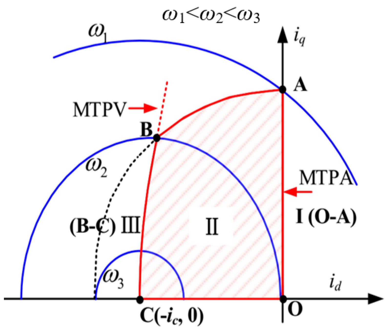
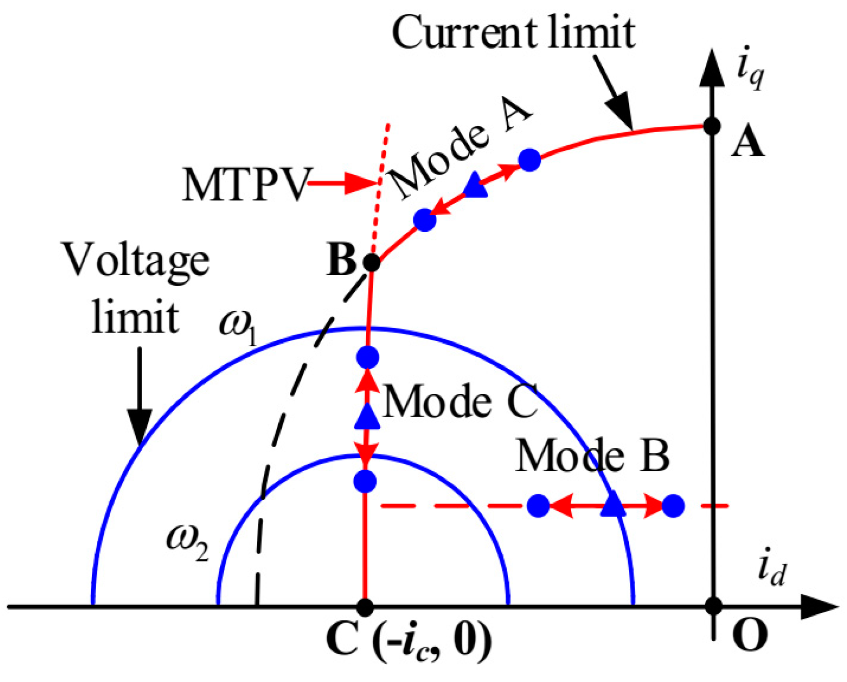
From (3), it can be seen that the voltage constraint is a circle whose center point is (${\omega }_e^2{L}_s{\psi }_m/Z_s^2$, ${\omega }_e{R}_s{\psi }_m/Z_s^2$) and the radius is $V_m/Z_s$. As the speed increases, the voltage limit circle shrinks. If the resistance is ignored or the machine speed is infinity, the center of the voltage limit circle is (−i_c, 0), where i_c is the characteristic current. As illustrated in Figure 1, the speed range of the machine with MTPV control can be categorized into three distinct regions:

1. Region I

In the region I, the machine operates on the curve ‘OA’, aiming to achieve maximum torque per ampere (MTPA). Since the machine operates inside the current and voltage limit circle, i.e., |I_s| < I_m and |V_s| < V_m, no flux-weakening control is required in this region.

2. Region II

The region II includes the curve ‘AB’ and the area within the closed curve ‘OABCO’. On the curve ‘AB’, the machine operates on the intersection point of the voltage and current limit circles, i.e., |V_s| = V_m and |I_s| = I_m. In the area ‘OABCO’, the machine operates on the voltage limit circle and inside the current limit circle, i.e., |V_s| = V_m and |I_s| < I_m. In region II, the flux-weakening control is required to satisfy the voltage and current constraints.

3. Region III

In the region III, the machine operates on the MTPV curve ‘BC’ that inside the current limit circle, i.e., |I_s| < I_m and |V_s| = V_m. In this region, the MTPV control strategy can be applied to maximize the torque capability and extend the operation speed range.

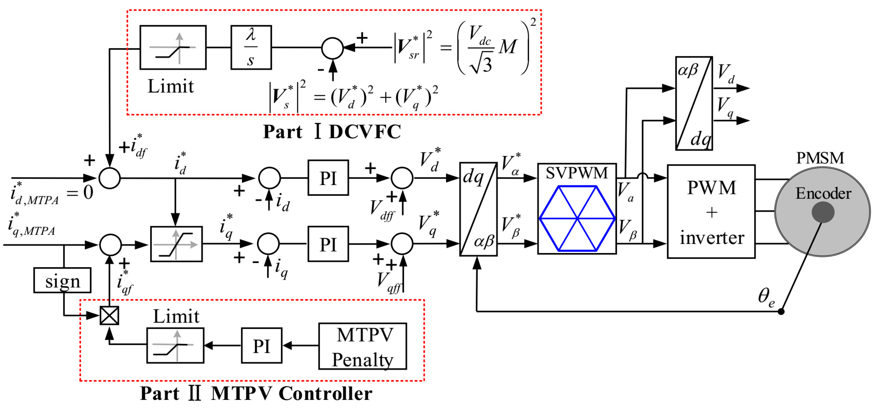
2.3. Control Strategies

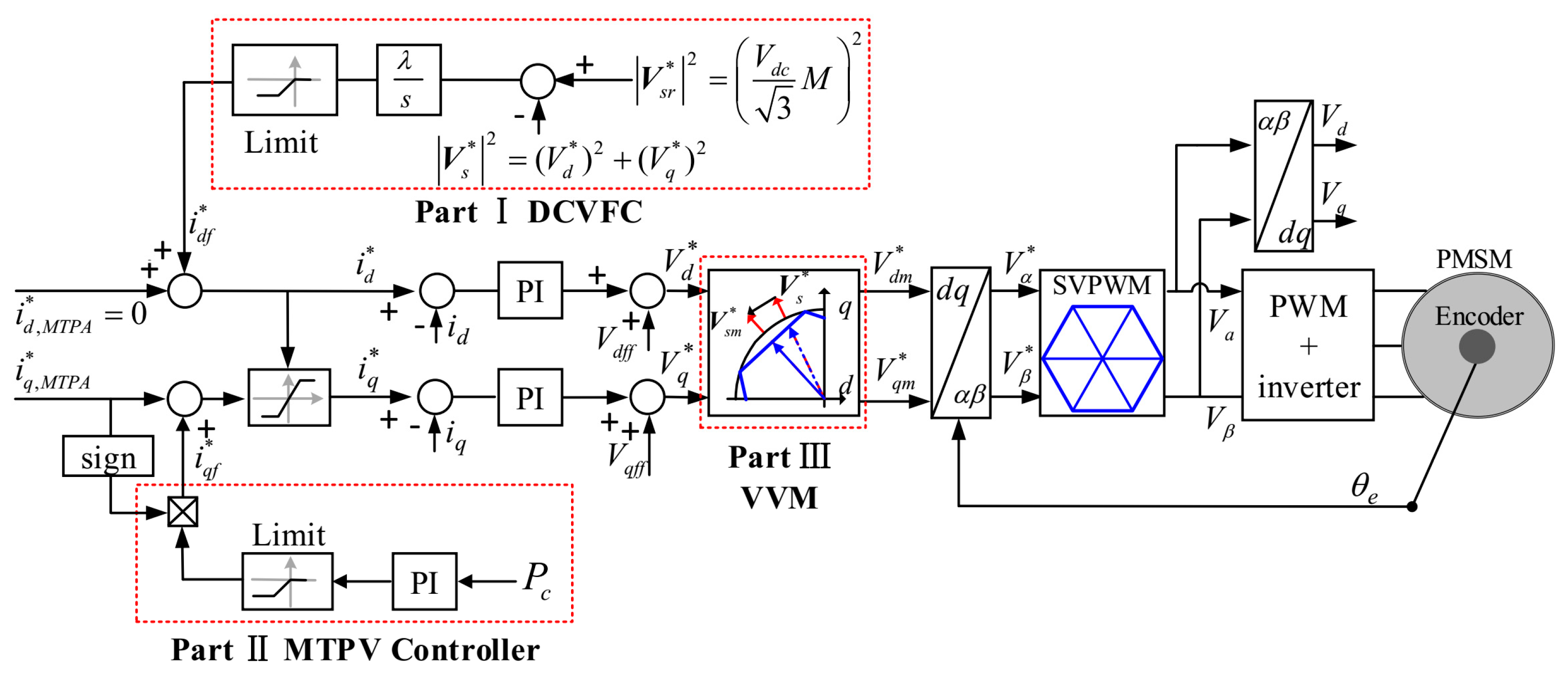
Figure 2 shows the schematic of the control system, which is based on the conventional current vector control system using a dual current control structure that regulates the i_d and i_q currents.

In the region I, d- and q-axis current commands, denoted as i^*_d,_MTPA and i^* _q,MTPA, are determined based on the MTPA method. For a non-salient PMSM, i^*_d,_MTPA is zero in the region I while i^*_q,_MTPA is directly calculated, as it is proportional to the torque requirement.

In region II, the d-axis current voltage feedback controller (DCVFC) using a pure integrator is applied [14]. The expression for the demagnetizing d-axis current command is given by

$$i_{df}^{*}=\lambda {\displaystyle \int ({\left|{\mathit{V}}_{sr}^{*}\right|}^2-{\left|{\mathit{V}}_s^{*}\right|}^2)}dt$$

(4)

where λ is the integration gain; i_df^* is the demagnetizing d-axis current command; V*_s is the voltage command vector before the over modulation block, i.e., (V_d^* + jV_q^*) in dq reference frame or (V_α^* + jV_β^*) in αβ reference frame; |V*_sr| is the voltage magnitude reference, i.e., $M{V}_{dc}/\sqrt{3}$, where M is the coefficient that can be used to adjust voltage magnitude reference. When M ≤ 1, the system operates in the LMR. For the conventional minimum phase error over modulation (MPEOM), when $M=2/\sqrt{3}$, the voltage magnitude can be extended to the hexagon boundary, at which condition the magnitude of the fundamental component is 0.6057 V_dc.

In the region III, the machine operates on the MTPV curve, which can be obtained at the tangent point of the voltage limit circle and constant torque curve. Therefore, the penalty function for the MTPV operation, i.e., P, can be defined as

$$P={\displaystyle \frac{1}{2}}({\displaystyle \frac{\partial {\left|{\mathit{V}}_s\right|}^2}{\partial i_d}}{\displaystyle \frac{\partial T_e}{\partial i_q}}-{\displaystyle \frac{\partial T_e}{\partial i_d}}{\displaystyle \frac{\partial {\left|{\mathit{V}}_s\right|}^2}{\partial i_q}})$$

(5)

where the condition P = 0 represents the MTPV curve. The MTPV control strategy is realized by designing a feedback controller that drives the penalty function to zero. This feedback-based approach ensures that the system automatically transitions from the FW region to the MTPV region. The feedback controller continuously monitors the system’s performance and makes real-time adjustments, seamlessly switching between the FW and MTPV regions, ensuring the machine operates efficiently on the MTPV curve. As shown in Part II of Figure 2, the q-axis current command is further modified by the output of a PI controller. The modified term, i.e., i_qf^*, can be expressed as

$$i_{qf}^{*}=sign(i_{q,MTPA}^{*})min(0,{\displaystyle \frac{k_{pqf}s+k_{iqf}}{s}}P)$$

(6)

where k_pqf and k_iqf are the proportional and integral gains of the PI controller. Therefore, the q-axis current command can be obtained as

$$i_q^{*}=sign(i_{q,MTPA}^{*})\min (\sqrt{I_m^2-{(i_d^{*})}^2},\left|i_{q,MTPA}^{*}+i_{qf}^{*}\right|)$$

(7)

The combined FW and MTPV controllers ensure efficient motor operation at high speeds in the MTPV region. The FW controller weakens the flux to enable higher speeds within voltage limits, while the MTPV controller adjusts i_q to maximize torque for the given voltage.

3. Optimized MTPV Controller

3.1. Penalty Function for MTPV

At steady state, by referring (1) and (5), P can be derived in voltage and current form as

$$P=\left\{\begin{array}{c}{P}_v={\omega }_e{V}_q{L}_s+R{V}_d\hfill \\ P_c=(i_d+i_c{\displaystyle \frac{{({\omega }_e{L}_s)}^2}{Z_s^2}})Z_s^2\hfill \end{array}\right.$$

(8)

where P_v and P_c represent the voltage and current forms of the penalty function, respectively.

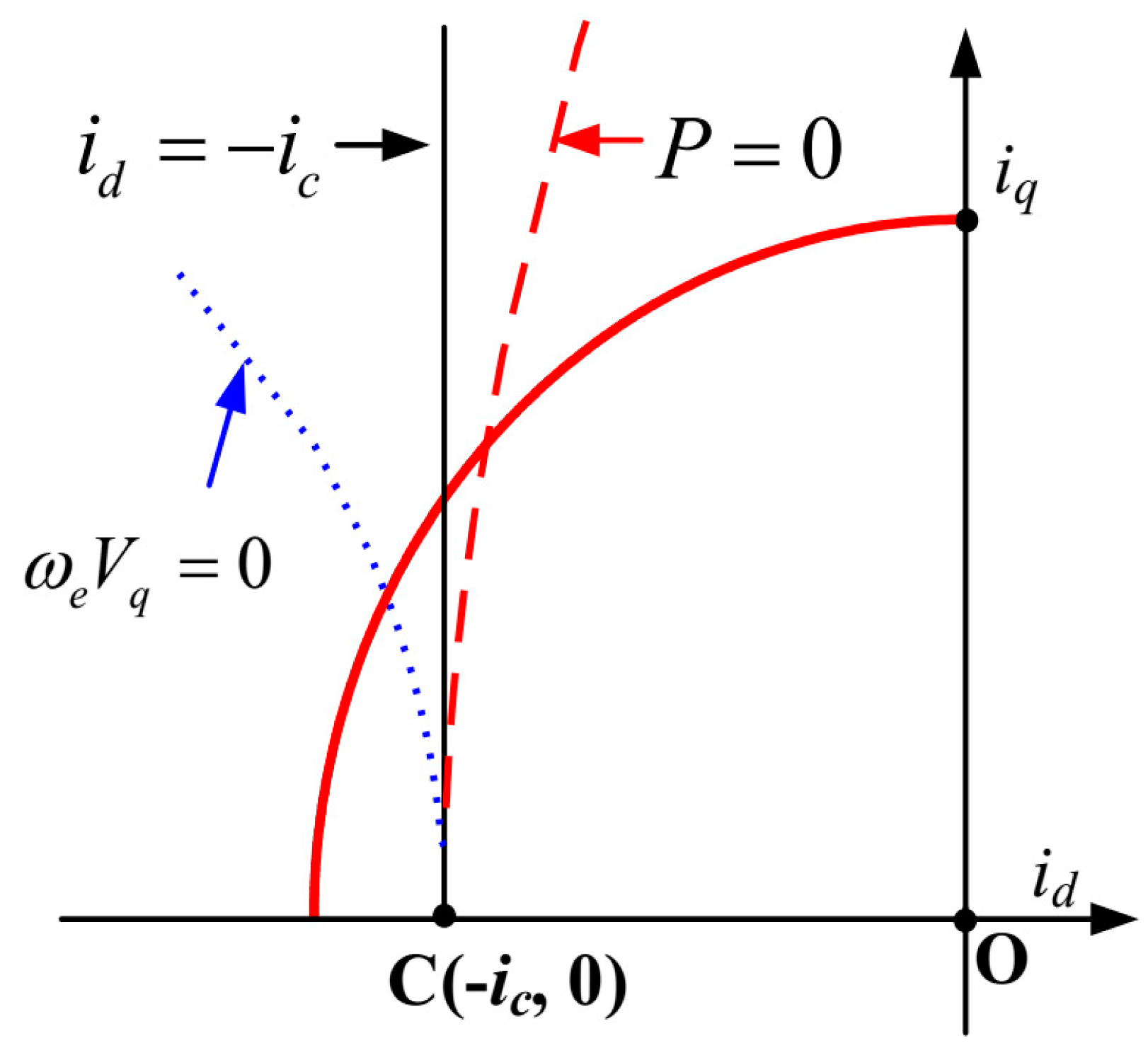
According to (8) if the resistance is ignored, the MTPV curve can be simplified as ω_eV_q = 0 or i_d = −i_c, as shown in Figure 3. However, for the small power machine especially when the power cable is required, the ignoring of the resistance could cause a notable deviation of the current trajectory from the actual one.

Thus, when seeking the optimal current trajectory, it is advantageous to employ a resistance-weighted penalty function. A voltage-based penalty term, P_v, can be defined in terms of the d- and q-axis voltage commands, V_d and V_q. However, in the over-modulation region, the over-modulation stage induces ripple components in both V_d and V_q. Furthermore, the voltage commands are not purely steady-state: they also include dynamic components arising from the output of the current PI regulator. For example, within the LMR, the q-axis voltage command satisfies V_q = V*_q (see Figure 2). Consequently, the PI regulator output V*_q is reintroduced into the q-axis current reference via the MTPV PI loop. Any high-frequency ripple on V*_q is therefore propagated—and even amplified—by the cascaded PI controllers. Because classical PI controllers offer limited rejection of such high-frequency components, this amplification can induce oscillations and, in the worst case, destabilize the drive. In [22], a precede first order low pass filter is added to the MTPV controller to solve this problem, and the penalty function is revised to P_vLpf, i.e.,

$$P_{vLpf}=P_v{\displaystyle \frac{{\omega }_c}{s+{\omega }_c}}$$

(9)

where ω_c is the cut off frequency of the lower pass filter. However, the introduced low pass filter will limit the dynamics of the MTPV loop. In order to improve the dynamic performance, the penalty function without low pass filter is preferred.

Alternatively, the penalty function can also be expressed in the current form, i.e., P_c, in (8). Since the MTPV controller aims to plan the current command trajectory in the region III, i_d in P_c can be replaced by the d-axis current command i_d^*. In addition, as P_c = 0 represents the MTPV curve, the term $Z_s^2$ can be canceled out. Therefore, the penalty function in the current form can be revised as

$$P_c=i_d^{*}+i_c{\displaystyle \frac{{({\omega }_e{L}_s)}^2}{Z_s^2}}$$

(10)

At the equilibrium point, the variation of the machine speed can be ignored due to the larger mechanical time constant when compared with the electrical time constant. Therefore, (10) implies that the variation of P_c mainly origins from the variation of i_d^*, i.e., ∆P_c = ∆i_d^*, where the prefix ‘∆’ denotes their corresponding small signals. From the small signal point of view, in ∆P_c, only ∆i_d^* is the information required for the MTPV control. According to (6), in region III, the d-axis current command output by DCVFC will be directly transformed to the q-axis current command by the MTPV controller. Therefore, no extra filter is required, and better dynamics can be expected than that by using the voltage command feedback MTPV controller.

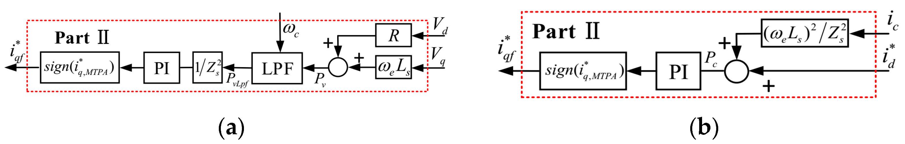
For easy comparison in the experimental section, the penalty function P_vLpf is divided by $Z_s^2$ to keep the same dimension as P_c in (10). The block diagrams of the MTPV controller by using voltage command feedback and current command feedback are shown in Figure 4a,b, respectively.

Since the optimal current trajectory for the MTPV requires accurate parameters, in practice, this could be done by online parameter estimation. As the parameter estimation is out of the scope of this paper, it will not be discussed further. It should be noted that accurate parameters are only required to improve the steady-state performance. Therefore, the parameters used for the estimating P_c can be updated much slower than the dynamics of the MTPV loop. It means that the MTPV control and parameter estimation will not interfere with each other if the penalty term P_c is employed. In other words, the improvement of the dynamic performance and the steady performance can be done separately. In this paper, P_c is finally used as the penalty function for the MTPV control owing to its better dynamic performance.

3.2. MTPV Control Design

Due to the nonlinear behavior of the voltage loop in flux-weakening regions, the flux-weakening controller can be designed based on the linearized model. Therefore, considering the current, voltage, and torque constraints, and according to the different small signal behaviors, the operation modes in the flux-weakening region can be classified into three categories, as shown in Figure 5: mode A, where the machine operates on the current limit circle; mode B, where the machine operates along the constant torque curve; and mode C, where the machine operates on the MTPV curve.

Under different operation modes, the direction of current variation differs and can be characterized by the slope of the current trajectory, defined as k = ∆i_q/∆i_d.

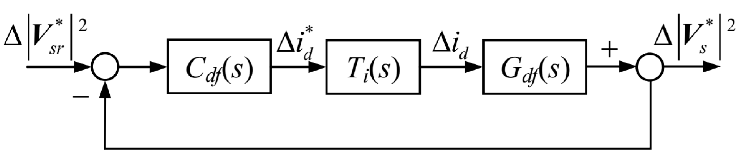
In region II, the MTPV controller is not activated, only the DCVFC is required. In region III, the DCVFC and MTPV controller are both involved in control, DCVFC is still an important part for the MTPV control. Therefore, DCVFC is analyzed first. Figure 6 shows the equivalent linearized model of the voltage loop with DCVFC [14]. In Figure 6, C_df(s), T_i(s) and G_df(s) are the transfer functions of the integral controller, the equivalent current loop, and the control plant, respectively. C_df(s), T_i(s) and G_df(s) can be expressed as

$$C_{df}(s)={\displaystyle \frac{\lambda }{s}}$$

(11)

$$T_i(s)={\displaystyle \frac{{\omega }_c}{s+{\omega }_c}}$$

(12)

$$G_{df}(s)={\displaystyle \frac{\mathsf{\Delta }{\left|{\mathit{V}}_s^{*}\right|}^2}{\mathsf{\Delta }{i}_d}}\approx {\displaystyle \frac{\mathsf{\Delta }{\left|{\mathit{V}}_s\right|}^2}{\mathsf{\Delta }{i}_d}}=2V_d^0{\displaystyle \frac{\mathsf{\Delta }{V}_d}{\mathsf{\Delta }{i}_d}}+2V_q^0{\displaystyle \frac{\mathsf{\Delta }{V}_q}{\mathsf{\Delta }{i}_d}}=bs+a$$

(13)

where ω_c is the bandwidth of the current loop; the variables with superscript ‘0’ denote their steady-state values on the equilibrium point.

Assuming ∆i_q = k∆i_d, a and b can be expressed as

$$\left\{\begin{array}{l}a=2{\omega }_e^0(V_q^0{L}_{\mathrm{s}}-V_d^{0}k{L}_s)+2R_s(V_d^0+V_q^{0}k)\\ b=2(V_d^0{L}_s+V_q^0{L}_{s}k)\end{array}\right.$$

(14)

Therefore, the close-loop transfer function of the voltage loop with DCVFC can be expressed as

$$\mathsf{\Phi }(s)={\displaystyle \frac{{\omega }_c\lambda (bs+a)}{s^2+{\omega }_c(1+b\lambda )s+{\omega }_c\lambda a}}$$

(15)

According to the Routh stability criterion, the stable condition of the voltage loop with DCVFC is

$$\left\{\begin{array}{c}a\lambda >0\hfill \\ 1+b\lambda >0\hfill \end{array}\right.$$

(16)

The details of selection of λ can be referred to Appendix A. When the machine operates in the region III, the operation mode B that is activated by the DCVFC cooperates with the mode C that is activated by the MTPV controller. For the DCVFC, the voltage loop can be analyzed in mode B. Since i_q remains constant in mode B, the slope k equals zero, and the coefficients a and b can be derived accordingly as

$$\left\{\begin{array}{c}{\left.a\right|}_{modeB}=2({\omega }_e^0{V}_q^0{L}_s+R{V}_d^0)\hfill \\ {\left.b\right|}_{modeB}=2V_d^0{L}_d\hfill \end{array}\right.$$

(17)

where a|_modeB and b|_modeB denote the values of a and b in mode B. At the equilibrium point, it can be seen that a|_modeB = 2P_v. Therefore, in the region III, a|_modeB = 0, which means that the voltage loop with DCVFC cannot maintain stable in this region and the MTPV control strategy has to be applied.

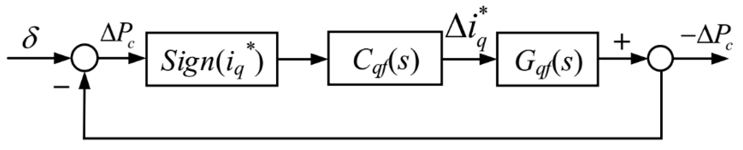
Furthermore, the equivalent linearized model of MTPV loop is shown in Figure 7. In Figure 7, C_qf(s) and G_qf(s) are the transfer functions of the PI controller and the control plant of the MTPV loop, respectively; δ is the reference of MTPV loop, which is an infinitesimal value. C_qf(s) and G_qf(s) can be obtained as

$$C_{qf}\left(s\right)={\displaystyle \frac{k_{pqf}s+k_{iqf}}{s}}$$

(18)

$$G_{qf}\left(s\right)=-{\displaystyle \frac{\mathsf{\Delta }{P}_c}{\mathsf{\Delta }{i}_q^{*}}}$$

(19)

According to (10), ∆P_c = ∆i* d, G_qf(s) can be rewritten as

$$G_{qf}\left(s\right)=-{\displaystyle \frac{\mathsf{\Delta }{i}_d^{*}}{\mathsf{\Delta }{i}_q^{*}}}$$

(20)

Since ∆i* d origins from DCVFC, G_qf(s) can be reconstructed as

$$G_{qf}\left(s\right)=-{\displaystyle \frac{\mathsf{\Delta }{i}_d^{*}}{\mathsf{\Delta }{\left|{\mathit{V}}_s^{*}\right|}^2}}{\displaystyle \frac{\mathsf{\Delta }{\left|{\mathit{V}}_s^{*}\right|}^2}{\mathsf{\Delta }{i}_q^{*}}}$$

(21)

In region III, the term $\mathsf{\Delta }{i}_d^{*}/\mathsf{\Delta }{\left|{\mathit{V}}_s^{*}\right|}^2$ can be obtained from Figure 6. When a = 0, it can be derived as

$${\displaystyle \frac{\mathsf{\Delta }{i}_d^{*}}{\mathsf{\Delta }{\left|{\mathit{V}}_s^{*}\right|}^2}}=-{\displaystyle \frac{\lambda }{s}}{\displaystyle \frac{(s+{\omega }_c)}{(s+{\omega }_c(1+{\left.b\right|}_{modeB}\lambda ))}}$$

(22)

According to Appendix A, b|_modeBλ ≈ 0 in region III, and $\mathsf{\Delta }{i}_d^{*}/\mathsf{\Delta }{\left|{\mathit{V}}_s^{*}\right|}^2\approx -{\lambda }_I/s$. In addition, $\mathsf{\Delta }{\left|{\mathit{V}}_s^{*}\right|}^2/\mathsf{\Delta }{i}_q^{*}$ can be derived as

$${\displaystyle \frac{\mathsf{\Delta }{\left|{\mathit{V}}_s^{*}\right|}^2}{\mathsf{\Delta }{i}_q^{*}}}=2V_d^0{\displaystyle \frac{\mathsf{\Delta }{V}_d^{*}}{\mathsf{\Delta }{i}_q^{*}}}+2V_q^0{\displaystyle \frac{\mathsf{\Delta }{V}_q^{*}}{\mathsf{\Delta }{i}_q^{*}}}$$

(23)

Moreover, since $V_q^0$ is close to zero, and $V_d^0=-V_{m}sign({\omega }_e^0{i}_q^{*})$ due to that i_d ≈ −i_c in region III, $\mathsf{\Delta }{\left|{\mathit{V}}_s^{*}\right|}^2/\mathsf{\Delta }{i}_q^{*}$ can be approximated as

$$\begin{array}{c}{\displaystyle \frac{\mathsf{\Delta }{\left|{\mathit{V}}_s^{*}\right|}^2}{\mathsf{\Delta }{i}_q^{*}}}\approx -2V_m{\displaystyle \frac{\mathsf{\Delta }{V}_d^{*}}{\mathsf{\Delta }{i}_q^{*}}}sign({\omega }_e^0{i}_q^{*})\hfill \\ \approx -2V_m{\displaystyle \frac{\mathsf{\Delta }{V}_d}{\mathsf{\Delta }{i}_q}}{\displaystyle \frac{\mathsf{\Delta }{i}_q}{\mathsf{\Delta }{i}_q^{*}}}sign({\omega }_e^0{i}_q^{*})=-2sign(i_q^{*})V_m\left|{\omega }_e^0\right|L_s{T}_i(s)\hfill \end{array}$$

(24)

In consequence, the control plant of the MTPV loop can be derived as

$$G_{qf}=K_{qf}{\displaystyle \frac{1}{s}}{T}_i(s)sign(i_q^{*})$$

(25)

where $K_{qf}=2V_m\left|{\omega }_e^0\right|L_s{\lambda }_I$. Equation (25) explains that a pure integral controller is not applicable for the MTPV controller, as the system could oscillate due to the resultant origin pole of the close-loop transfer function. Therefore, a PI controller can be adopted, which can ensure the stability in region III. The open-loop transfer function of the MTPV loop with PI controller, i.e., G_oqf(s) can be derived and simplified as

$$G_{oqf}=K_{qf}{\displaystyle \frac{k_{pqf}s+k_{iqf}}{s}}{\displaystyle \frac{1}{s}}{T}_i(s)$$

(26)

It is reasonable to make a further simplification of (26) by approximating T_i(s) as a unity gain if the MTPV loop is tuned with the bandwidth much lower than the current bandwidth. Therefore, the close-loop function of the MTPV loop can be obtained as

$${\displaystyle \frac{-P_c}{\delta }}={\displaystyle \frac{(k_{pqf}{K}_{qf}s+K_{qf}{k}_{iqf})}{s^2+k_{pqf}{K}_{qf}s+K_{qf}{k}_{iqf}}}$$

(27)

As a second order system, the control parameters can be tuned as

$$k_{pqf}={\displaystyle \frac{2\xi {\omega }_{Nqf}}{K_{qf}}}={\displaystyle \frac{2{\omega }_{Nqf}}{K_{qf}}},k_{iqf}={\displaystyle \frac{{\omega }_{Nqf}^2}{K_{qf}}}$$

(28)

where ω_Nqf is the selected natural frequency, ξ is selected damping factor which is set at 1 in the experiments.

3.3. Over Modulation Improvement

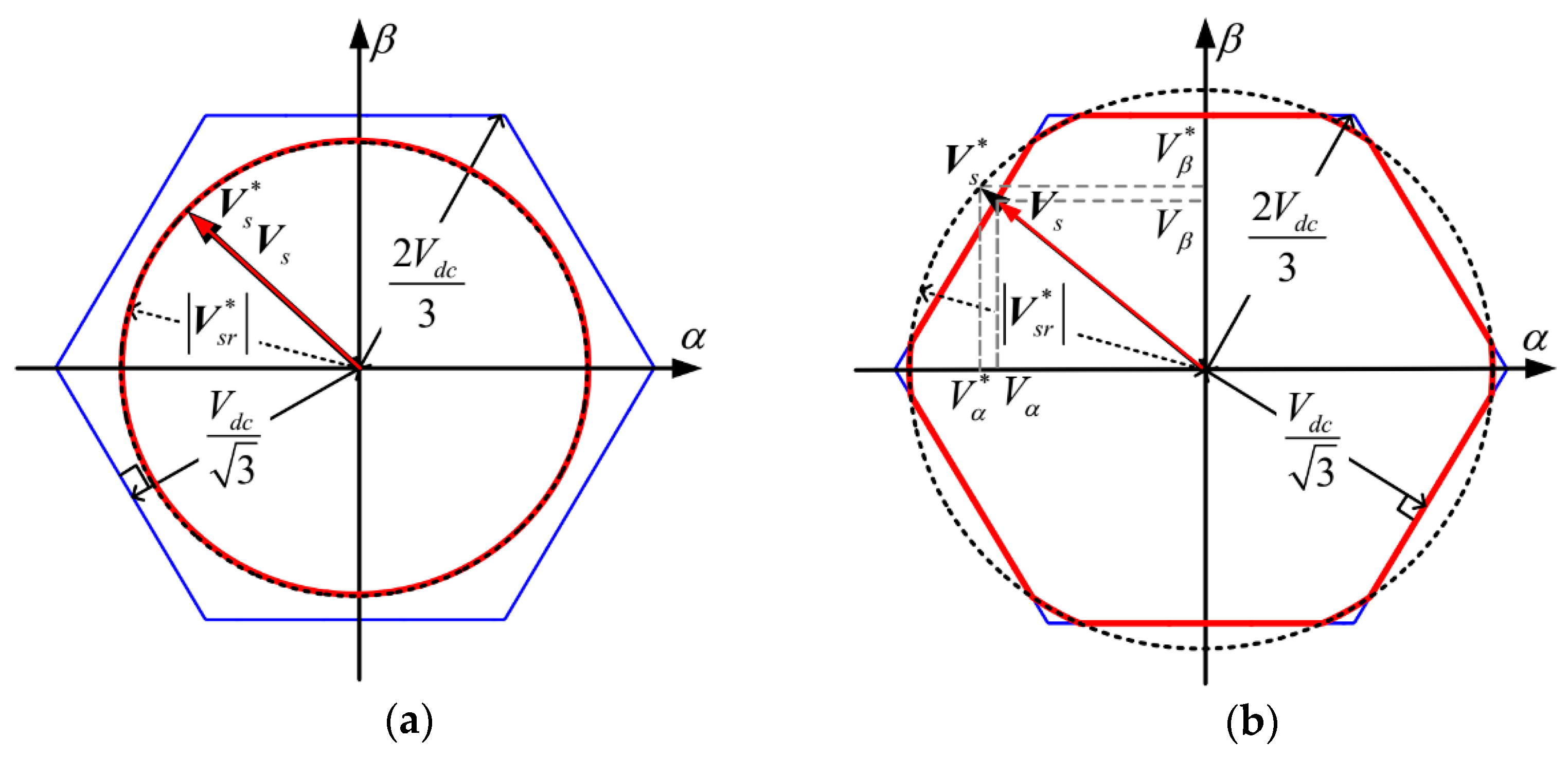
Figure 8 illustrates voltage synthesis under MPEOM in both linear and over-modulation regions. In the linear region, the reference voltage vector V_s can be accurately synthesized without distortion. However, in the over-modulation region, only vectors located within the hexagonal boundary are fully realizable. Any reference vector extending beyond this limit is clipped to the hexagon perimeter while preserving its direction. 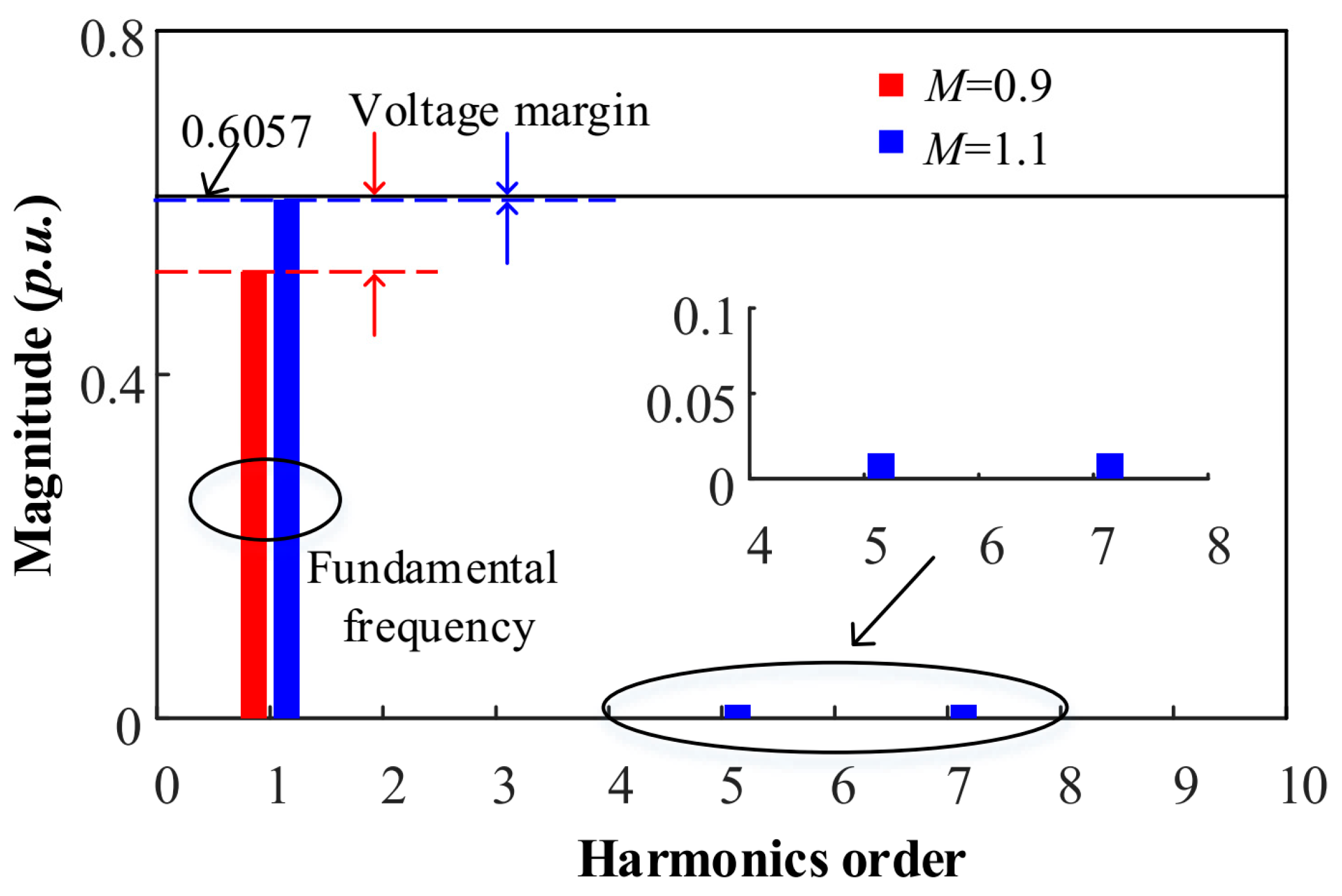Figure 9 presents the normalized spectral content of the α-axis voltage with respect to V_dc for modulation indices M = 0.9 and M = 1.1. The amplitude of the fundamental component serves as an indicator of DC-link voltage utilization.

The over-modulation region demonstrates improved utilization of the DC-link voltage compared to the LMR. However, this benefit comes at the cost of reduced voltage control margin and increased harmonic content. As a result, voltage saturation becomes more prominent, negatively impacting current regulation and potentially causing instability. To mitigate this issue, the flux-weakening control scheme utilizes a d-axis current reference generated via the DCVFC and a q-axis current reference provided by the MTPV controller. Ensuring rapid and stable current dynamics is thus critical for maintaining system stability within the flux-weakening region.

In the over modulation region, the VVM shows a good option for improving the current dynamics, which is firstly proposed in [9] and applied in region II. In this paper, the VVM will be applied in both region II and region III to improve the system stability in over modulation region. The working principle of the VVM is quite simple, which will be briefly introduced as follows.

Since the inductive voltage drop on the inductance can be approximated as

$$\left\{\begin{array}{c}{L}_s{\displaystyle \frac{d{i}_d}{dt}}\approx V_d+{\omega }_e{L}_s{i}_q\hfill \\ L_s{\displaystyle \frac{d{i}_q}{dt}}\approx V_q-{\omega }_e(L_s{i}_d+{\psi }_m)\hfill \end{array}\right.$$

(29)

The right side of (29) represents the voltage margin in d- and q-axes that can be created. When V_d and V_q are already limited on the hexagon boundary, the only way to increase the voltage margin is to utilize the coupling term between d- and q-axes. 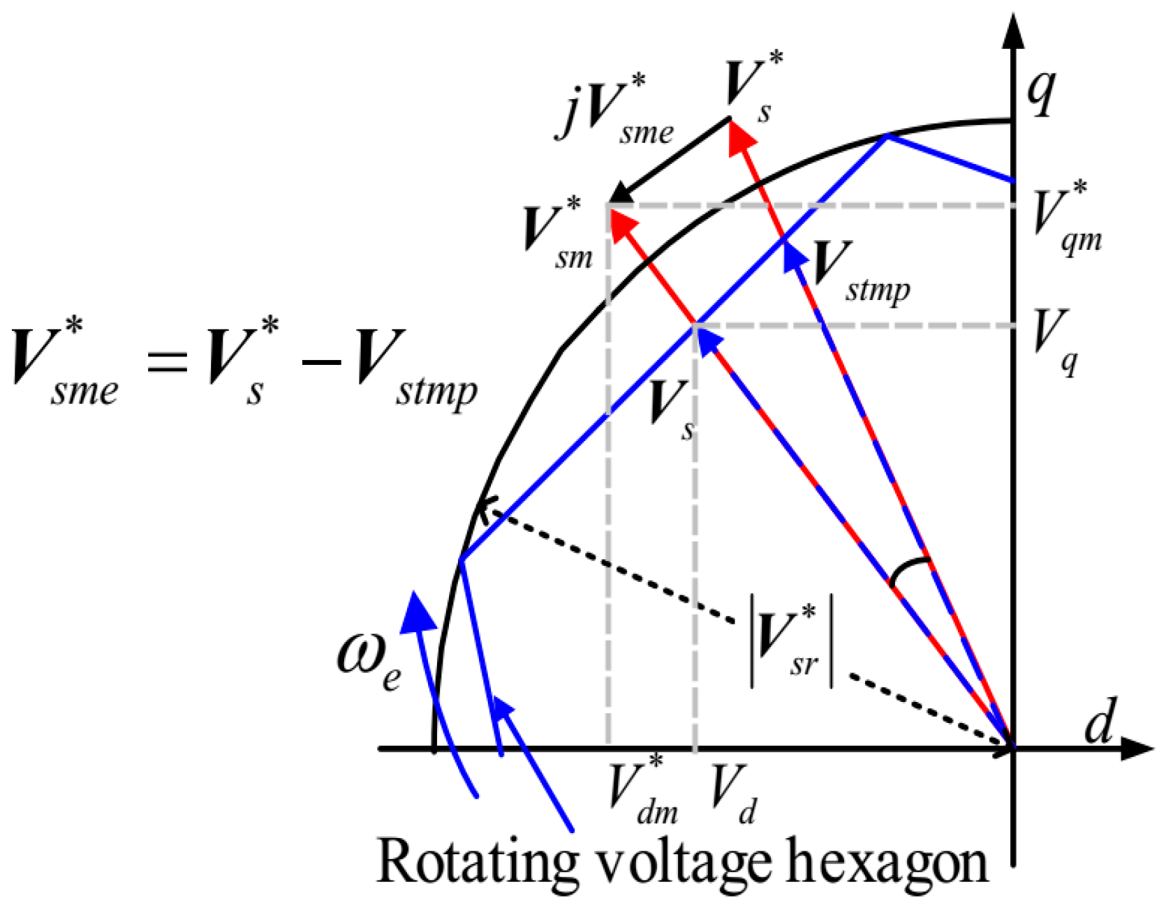For example, when ω_e > 0, decreasing i_d can be realized by decreasing i_q, and therefore decreasing V_q; increasing i_q can be realized by decreasing i_d, and therefore decreasing V_d. By utilizing this coupling feature between d- and q-axes, the voltage command vector can be modified as

$${\mathit{V}}_{sm}^{*}={\mathit{V}}_s^{*}+j{\mathit{V}}_{sme}^{*}\mathrm{sign}({\omega }_e)$$

(30)

where V^*_sme = V^*_s – V_stmp is the temporal voltage error vector between the input voltage command vector V^*_s and temporal voltage vector V_stmp, as shown in Figure 10; V^*_sm is the new modified voltage vector, i.e., V^*_dm + j V^*_qm.

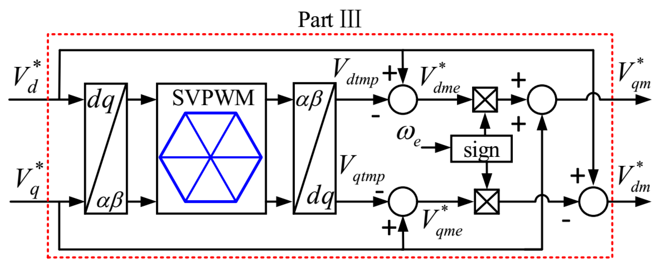
Figure 11 presents the scalar-based implementation of the VVM in block diagram form. In this configuration, the voltage commands generated by the current controllers, V_d^* and V_q^* are modified to V_dm^* and V_qm^*, through the VVM. These modified commands are subsequently processed by the MPEOM scheme before being applied to the inverter.

The whole control diagram with MTPV controller and the VVM can be seen in Figure 12. Since the temporal voltage error vector V^*_sme only exists in the over modulation region, the VVM will not influence the steady-state performance in the LMR.

4. Experimental Verification

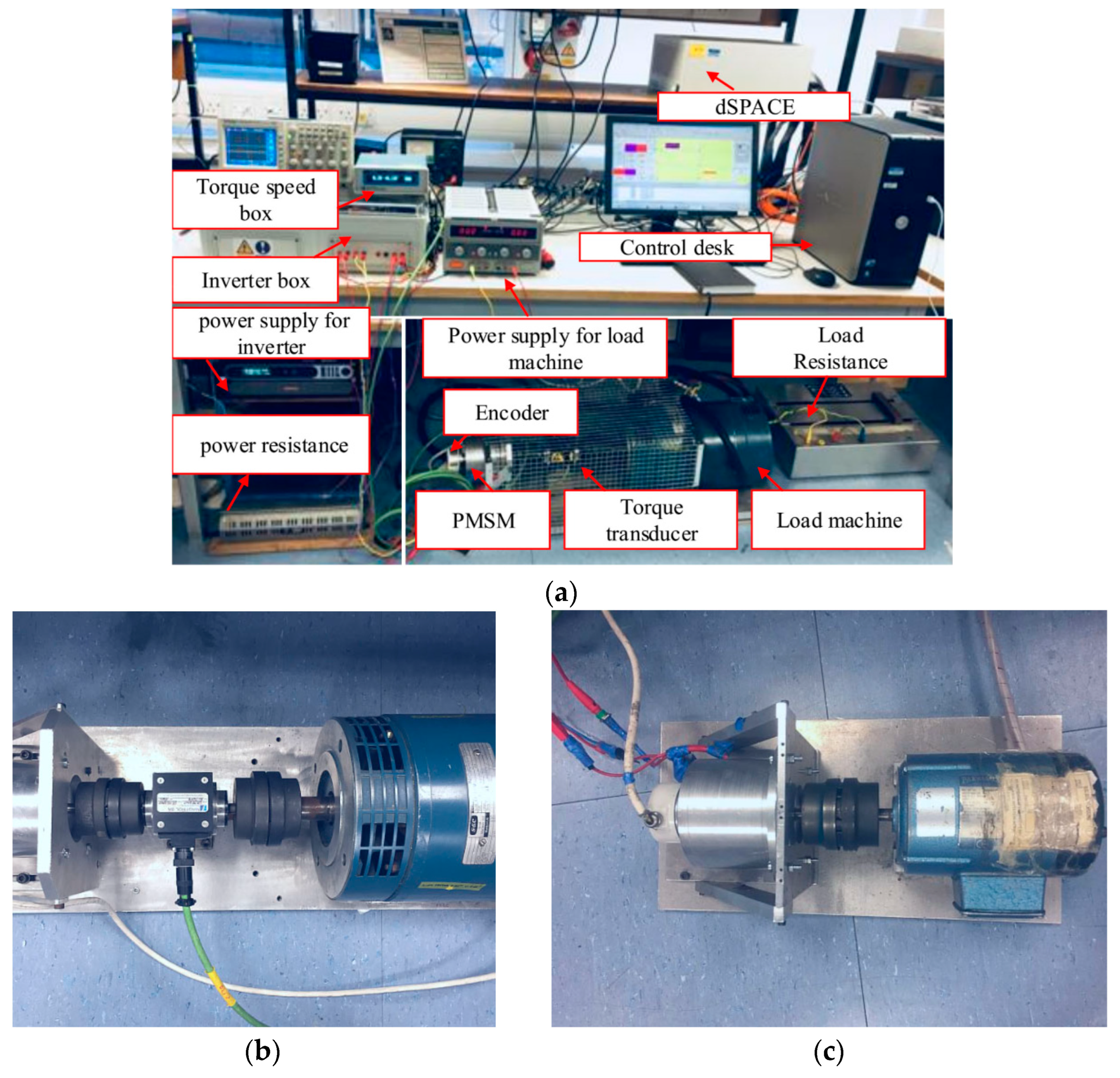
Experimental validation is carried out using a non-salient pole PMSM controlled via a dSPACE-based setup. The inverter employs IRFH7440-type MOSFETs as switching devices. Due to its negligible value relative to the motor resistance, the drain-source resistance (below 2.4 mΩ) is disregarded in analysis. The system operates at a PWM switching frequency of 10 kHz, with the current control loop bandwidth configured at 1200 rad/s. A visual overview of the experimental setup is provided in Figure 13.

As shown in Figure 13, Test Rig I is equipped with a high-inertia load of 0.012 kg·m² and incorporates a torque transducer for steady-state performance evaluation. In contrast, Test Rig II features a lower inertia of 0.001 kg·m², making it suitable for assessing transient behavior. Detailed specifications of the machine and drive system are provided in

Table 1. Machine and drive parameters.

Parameters	Value
Phase resistance (Rs)	0.25 Ω
Synchronous inductance (Ls)	1.7 mH
PM-flux linkage (ψm)	10 mWb
Number of pole pairs	10
DC link voltage (Vdc)	14 V
Current limit (Im) when icn = 1	7.35 A
Current bandwidth (ωcc)	1200 rad/s
Rated speed (n*)	1000 rpm
Cable resistance	0.1 Ω
PWM switching frequency	10 Hz

. For dynamic testing, data acquisition is conducted at a sampling rate of 1 kHz.

The following experimental results begin with an evaluation of steady-state performance using Test Rig I, highlighting the benefits of incorporating resistance effects within the MTPV region. Subsequently, the dynamic behavior of the system employing a current command feedback MTPV controller is examined and compared against its voltage command feedback counterpart. Finally, system stability in the over-modulation region is analyzed under conditions with and without the implementation of the VVM.

4.1. Steady-State Performance

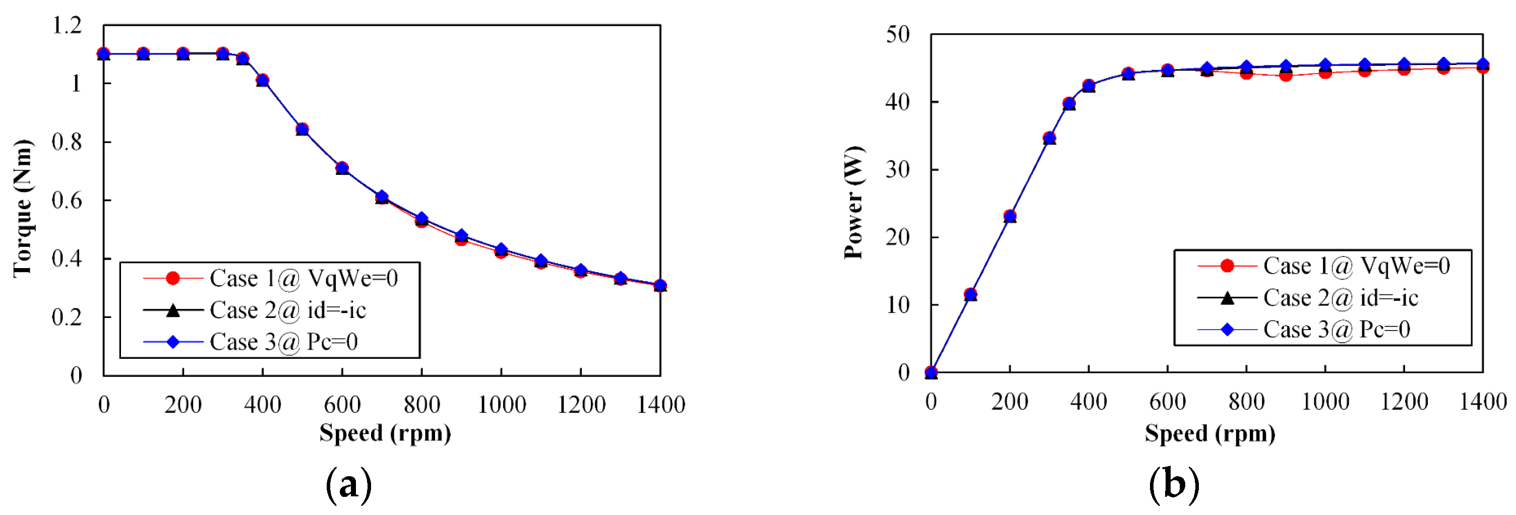
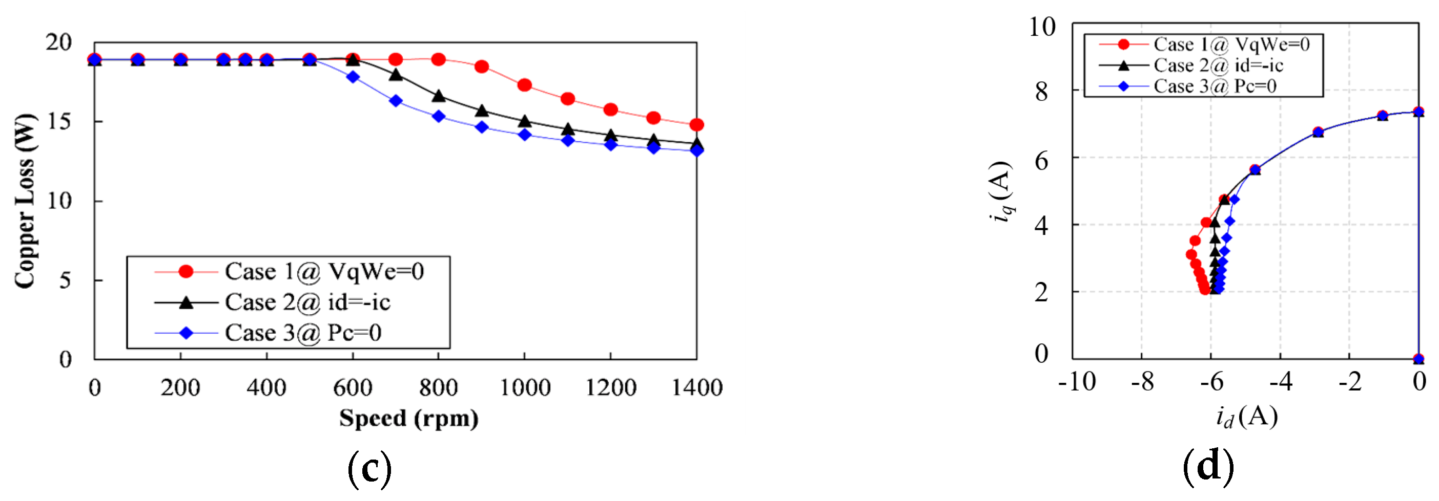
Figure 14 shows the steady-state performance for M = 0.9M under three distinct MTPV penalty function scenarios: V_qω_e = 0 (case 1) i_d = −i_c (case 2) and P_c = 0 (case 3). Cases 1 and 2 correspond to implementations where the impact of resistance is neglected, using voltage- and current-based forms, respectively. In contrast, Case 3 incorporates the resistance effect into the penalty function. The resistance value considered in P_c is the total resistance of the system, set to 0.35 Ω.

Figure 14a,b show the torque speed curve and power speed curve, respectively, under three cases. Although the variations in output torque and power among the three test cases are relatively small, Case 3 consistently delivers marginally higher values compared to Cases 1 and 2 when the machine speed exceeds approximately 650 rpm. Conversely, Case 1 produces the lowest torque and power across the range. As illustrated in Figure 14c, Case 3 also exhibits the lowest copper losses among the three scenarios. At 900 rpm, the copper loss in Case 3 is approximately 25% lower than that of Case 1. Figure 14d further reveals that Case 3—where resistance is taken into account—achieves the smallest current magnitude, particularly near the operating region where the system transitions from mode A to mode C, thereby contributing to the reduced copper loss. Additionally, Case 3 enters the MTPV region earlier than the others. Accurate tracking of the MTPV trajectory during dynamic transitions may further enhance the system's dynamic response.

4.2. Dynamic Performance with Different MTPV Controllers

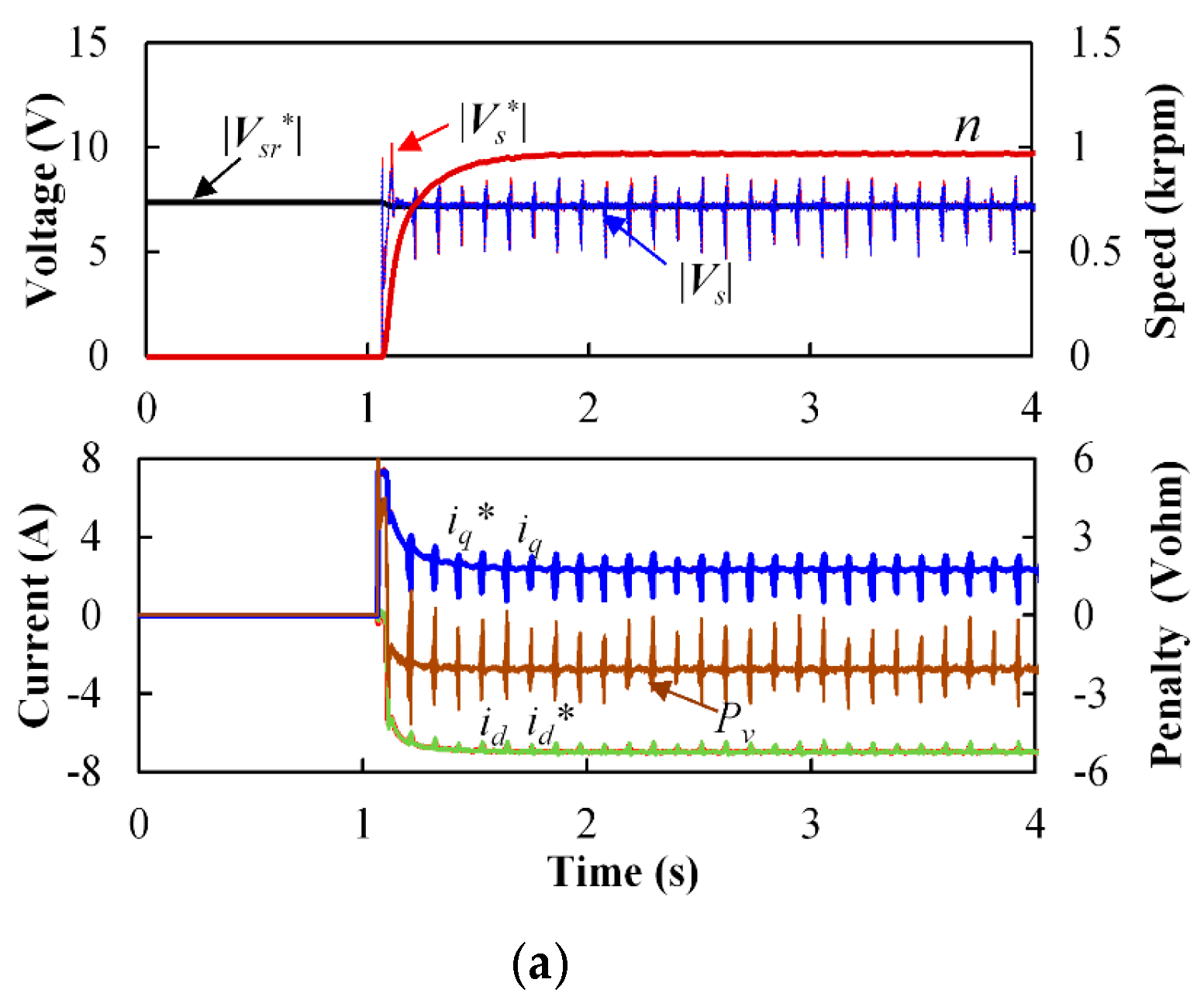
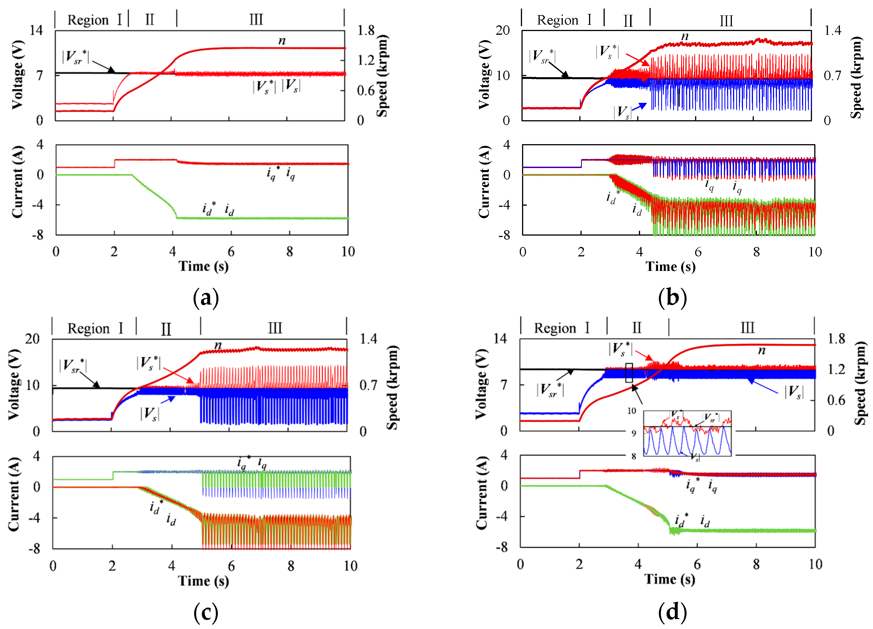
The dynamic responses of the system under voltage and current command feedback MTPV control schemes are evaluated by applying a step input of i^*_q,MTPA = 7.35A with a modulation index M = 0.9. Figure 15 shows the dynamic behavior of the system using the voltage command feedback controller under varying PI parameter settings. In Figure 15a, noticeable oscillations occur in the absence of a low-pass filter. By setting ω_Nqf = 50 rad/s and ω_c = 600 rad/s, the system maintains stable behavior, as depicted in Figure 15b, though an evident overshoot appears in both the current response and the and P_vLpf profile. When the cutoff frequency ω_Nqf is increased further—as shown in Figure 15c—oscillatory behavior reemerges, indicating a loss of system stability.

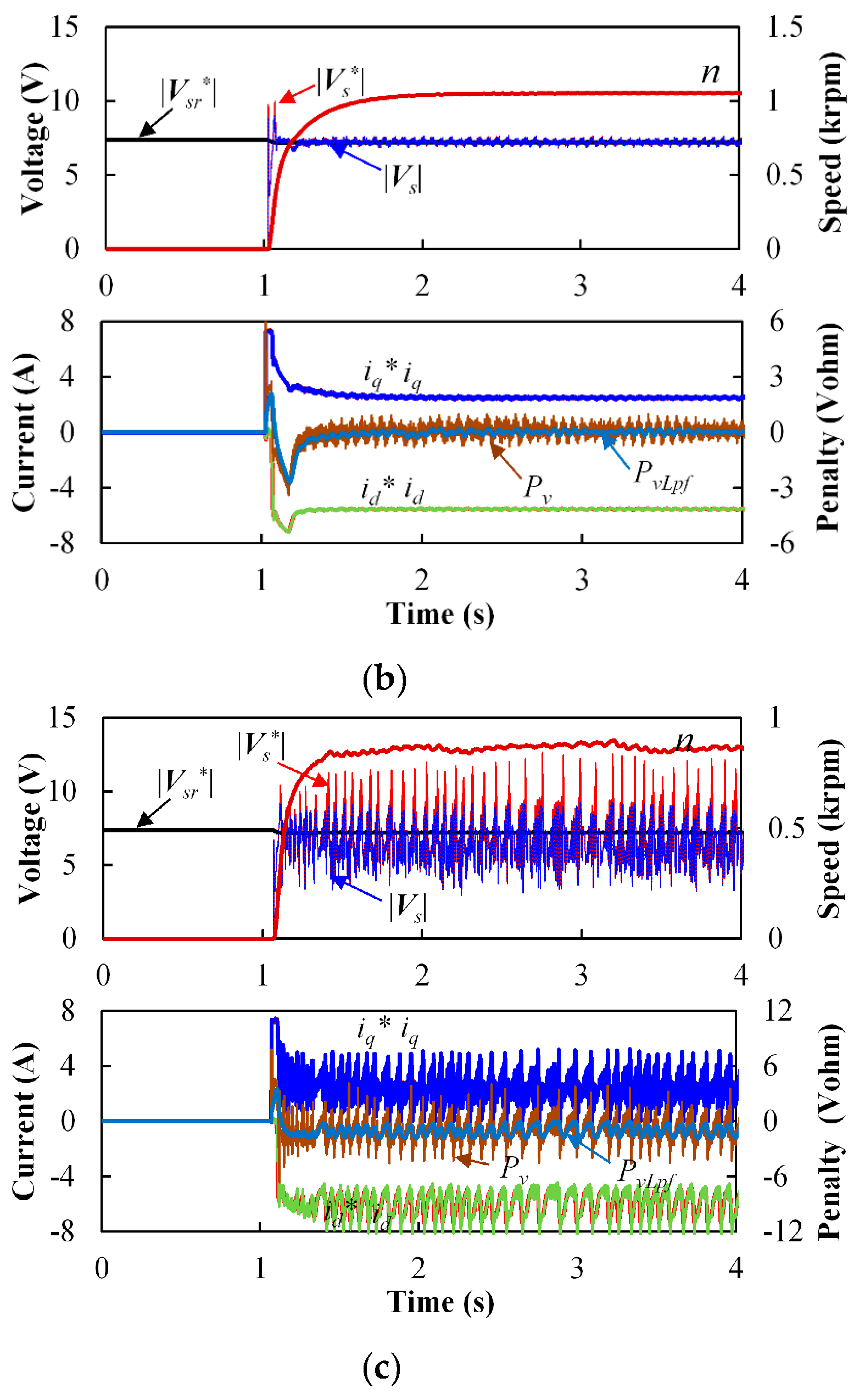
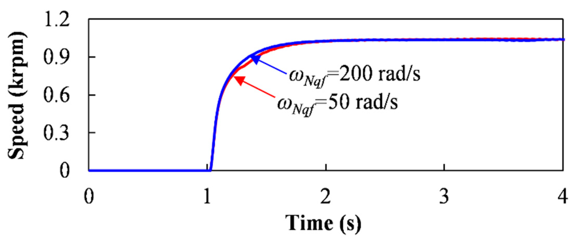
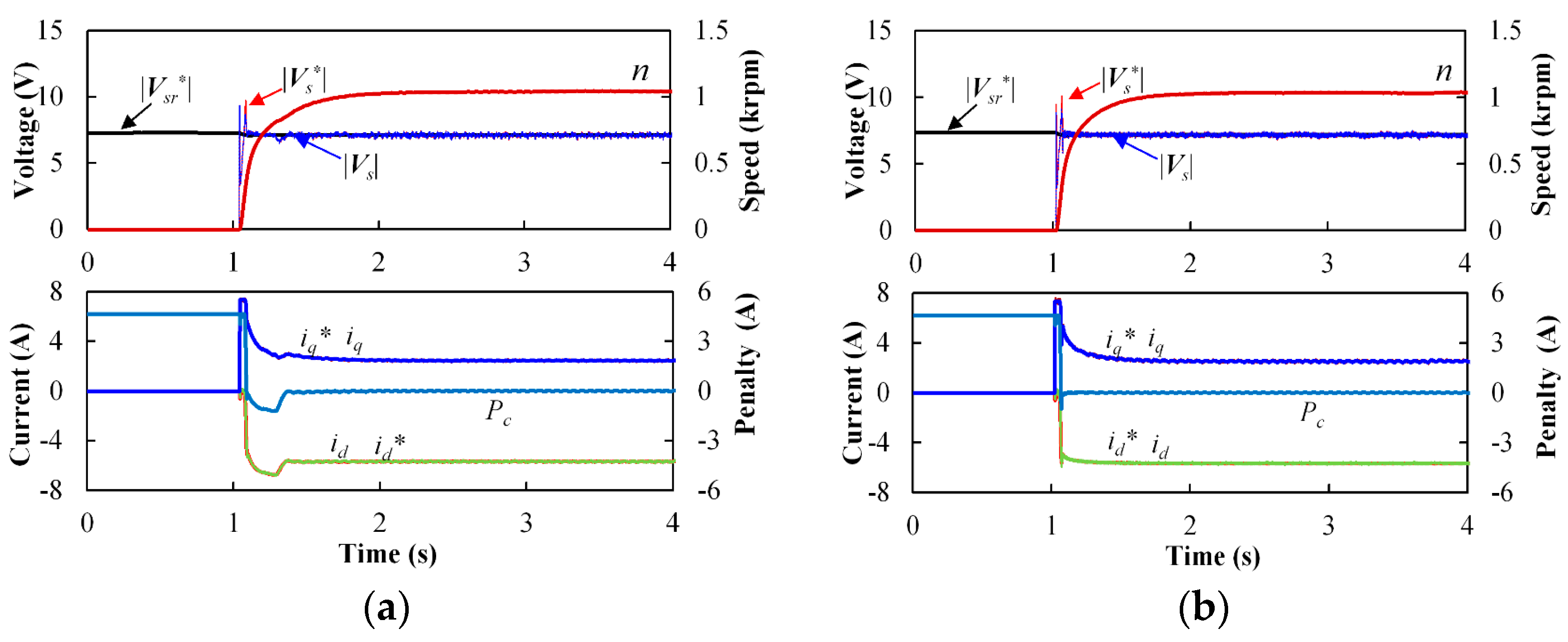
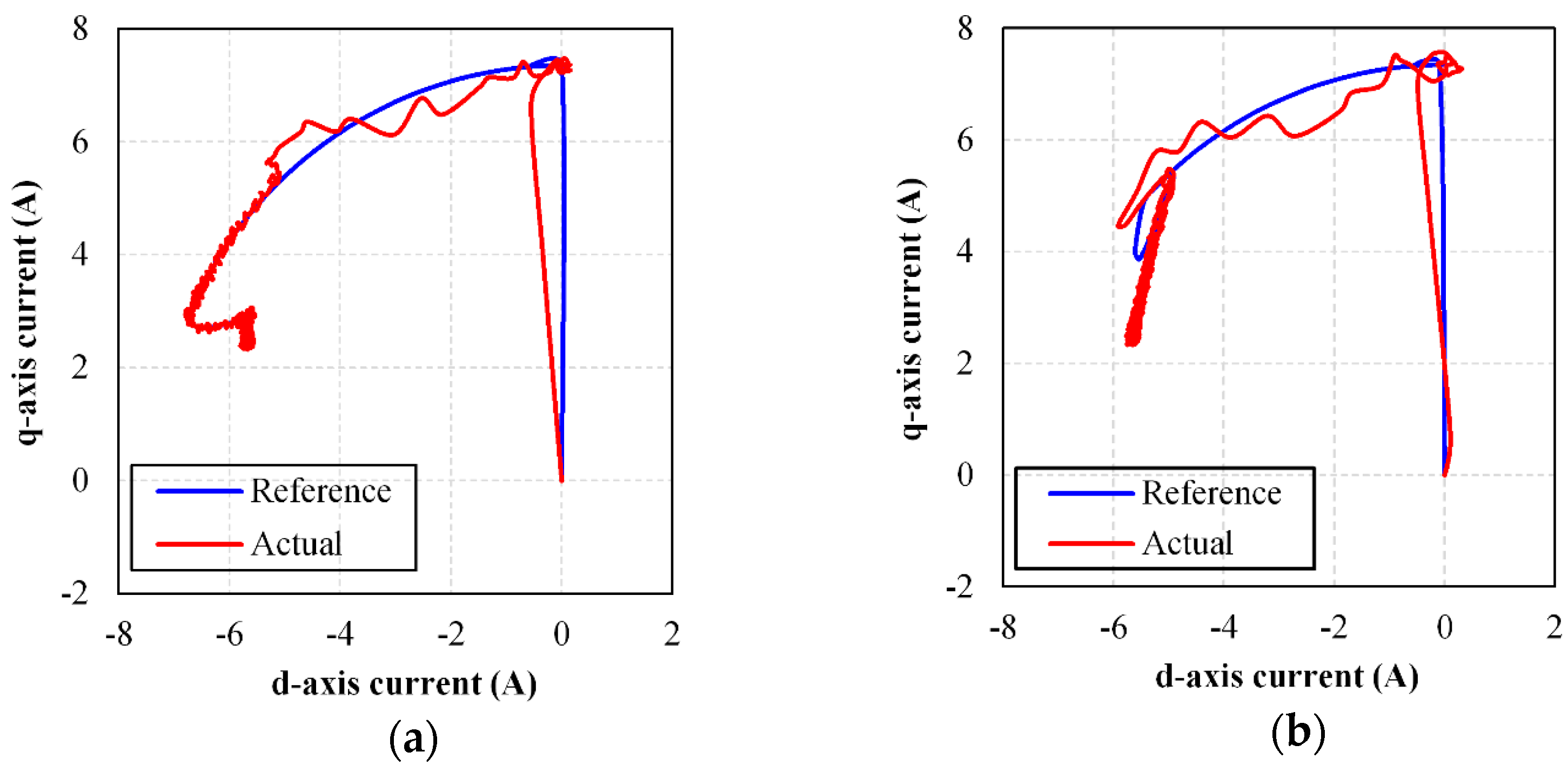
Figure 16 shows the dynamic performance by using the current command feedback MTPV controller under different PI control parameters. It can be seen that the system can operate stably when ω_Nqf are 50 rad/s and 200 rad/s, as shown in Figure 16a,b, respectively. Figure 17 illustrates the current trajectories when ω_Nqf = 50 rad/s and 200 rad/s. when ω_Nqf = 50, as shown in Figure 17a, although the current shows overshoot when approaching MTPV curve, this overshoot is much less when ω_Nqf increases to 200 rad/s. As a result, better speed dynamics can be obtained, which can be seen in Figure 18.

From the foregoing analysis, the pure integral MTPV controller can hardly maintain the stability in the MTPV region. In order to demonstrate this phenomenon, Figure 19 shows one of the oscillation cases when the integral gain is tuned by disabling the proportional controller while ω_Nqf = 50 rad/s.

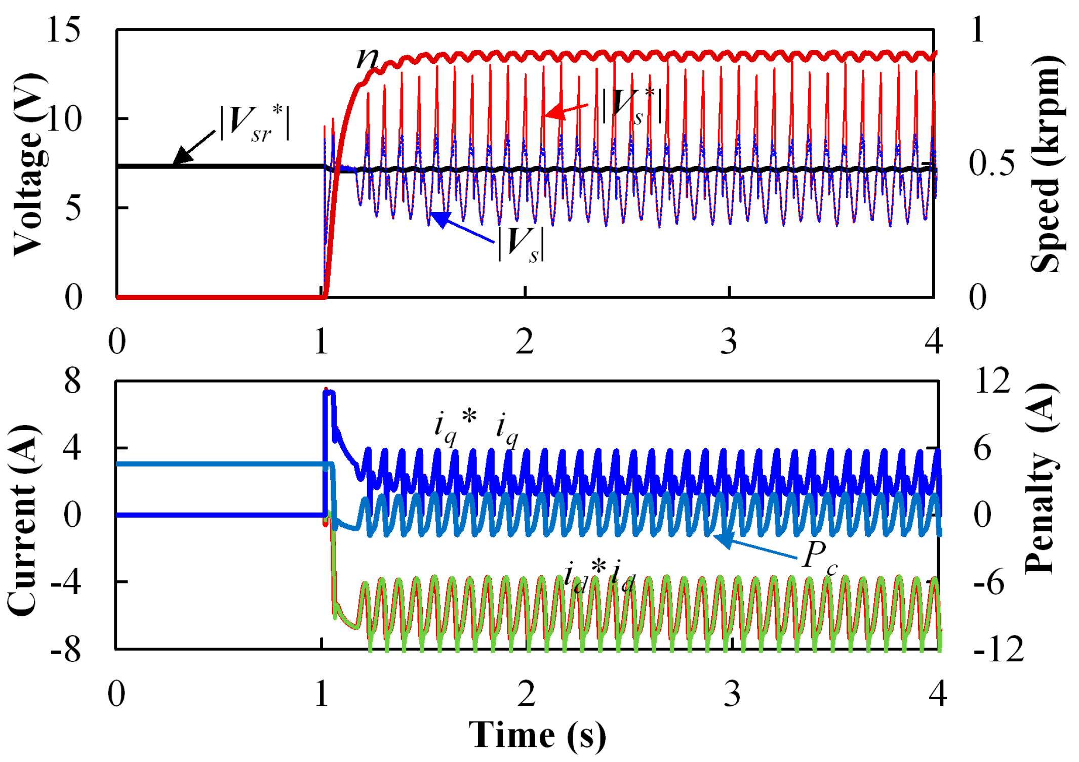
4.3. Stability in over Modulation Region

When M = 1.15, the system stabilities are compared under the conditions with and without VVM. By changing q-axis current command from 1A to 2A at 2 seconds, the machine accelerates from region I to region II, and then to region III. Figure 20a shows the system performance without VVM. It can be seen that both current and voltage oscillate in the flux-weakening regions (region II and region III). However, as shown in Figure 20b, with the VVM, the system stability in flux-weakening region is remarkably improved. It should be noted that the ripples of |V_s| in Figure 20b is caused by the limit boundary of the over modulation block.

5. Conclusions

This paper investigates and improves a feedback-oriented flux-weakening control scheme for a non-salient PMSM, with particular emphasis on its operation in the MTPV region. To improve steady-state performance—particularly in low-power machines—the effect of stator resistance has been incorporated into the control framework. A comparative study of two MTPV controller structures, namely voltage-command and current-command feedback controller, has been conducted. Additionally, design considerations for a PI-based MTPV controller have been addressed with respect to maintaining system stability in the MTPV region. To further enhance system robustness in both over-modulation and flux-weakening regions, a VVM is employed. Theoretical analysis and experimental validation confirm the effectiveness of the proposed methods, demonstrating that:

1. The steady-state performance in the MTPV region can be improved by considering the resistance especially for the small power machine;

2. The current command feedback MTPV controller can obtain better dynamics than the voltage command feedback controller;

3. A PI MTPV controller is preferred as the pure integral MTPV controller can hardly maintain stability in the MTPV region;

4. The stability in the over modulation region under different flux-weakening regions (region II and region III) can be improved with VVM while the dual current control structure can still be preserved.