Compressed Air Energy Storage in Salt Caverns Optimization in Southern Ontario, Canada

Abstract

Energy storage systems are gaining increasing attention as a solution to the inherent intermittency of renewable energy sources such as solar and wind power. Among large-scale energy storage technologies, compressed air energy storage (CAES) stands out for its natural sealing properties and cost-efficiency. Having abundant salt resources, the thick and regionally extensive salt deposits in Unit B of Southern Ontario, Canada, demonstrate significant potential for CAES development. In this study, optimization for essential CAES salt cavern parameters are conducted using geological data from Unit B salt deposit. Cylinder-shaped and ellipsoid-shaped caverns with varying diameters are first simulated to determine the optimal geometry. To optimize the best operating pressure range, stationary simulations are first conducted, followed by tightness evaluation and long-term stability simulation that assess plastic and creep deformation. The results indicate that a cylinder-shaped cavern with a diameter 1.5 times its height provides the best balance between storage capacity and structural stability. While ellipsoid shape reduces stress concentration significantly, it also leads to increased deformation in the shale interlayers, making them more susceptible to failure. Additionally, the findings suggest that the optimal operating pressure lies between 0.4 and 0.7 times the vertical stress, maintaining large capacity and minor gas leakage, and developing the least creep deformation.

1. Introduction

Nowadays, the global energy landscape is undergoing a significant transformation, driven by increasingly severe climate change and energy shortage. Since 2010, global warming has accelerated by more than 50% over the 1970–2010 warming rate of 0.18 °C per decade [1]. Additionally, 1.6 billion people are in threat of energy shortage, with the world’s population projected to reach 8.6 billion by 2030 [2]. These escalating situations necessitate an urgent shift from traditional fossil fuels to renewable and cleaner energy sources, including but not limited to wind, solar, geothermal, and hydropower. Such energy sources have been vigorously developed worldwide. By 2030, renewable electricity generation worldwide is projected to surpass 17,000 TWh, which is an increase of nearly 90% from 2023 levels, and solar photovoltaic technology is expected to drive approximately 80% of this growth [3]. Governments are increasingly committed to adopting renewable energy sources. Japan aims to increase its renewable energy share to up to half of the country’s electricity needs by 2040, reducing greenhouse gas emissions by 70% from 2013 levels within the next 15 years, targeting carbon neutrality by 2050 [4]. In 2024, Europe achieved a milestone with 47% of its electricity generated from renewable sources like solar and wind. The European Union aims to achieve a 55% reduction in emissions by 2030 and become the first climate-neutral continent by 2050 [5].

Currently, the development of renewable energy faces technical bottlenecks, as mainstream renewable energy sources generally suffer from intermittent power supply issues, with their output constrained by seasonal and climatic conditions. For example, in December 2024, German consumers faced electricity prices averaging EUR 395 per MWh, the highest since December 2022, caused by low wind and solar power generation due to adverse winter weather conditions. The wind power generation fell from an average capacity of nearly 20 GW to just over 3 GW, challenging the overall stability of the energy grid [6]. The construction of energy storage systems can effectively address the issue of intermittency. Such systems can adapt to the random fluctuations in power systems by storing excess electricity during periods of peak generation and releasing it when power supply is insufficient. Extensive research has been conducted to explore the application of energy storage systems. Malka et al. analyzed the feasibility of integrating energy storage systems into Albania’s Drin River Cascade hydropower plants to reduce energy losses, manage transmission congestion, and improve renewable energy integration [7]. Zou et al. analyzed how China’s electricity market evolves with increasing renewable energy integration under the 2050 High Renewable Energy Penetration Roadmap, find out that energy storage systems stabilize electricity prices and reduce ancillary service costs [8]. Evans et al. evaluated and compared various energy storage technologies to address the intermittency of renewable energy sources and ensure a stable electricity supply for utility-scale applications [9].

Large-capacity energy storage systems include pumped hydro energy storage (PHES), geothermal energy storage (GES), hydrogen storage, and compressed gas energy storage (CAES) [10]. PHES is the most mature technology, with decades of operational experience. However, such a system is constrained by specific topographical features. Moreover, construction of a such system can impact local ecosystems and may involve significant land use [11]. GES harnesses natural underground heat resources, thus avoiding the influence of weather conditions and providing a more stable and continuous energy output. Nevertheless, GES implementation requires specific geological conditions, and initial preparation like exploration and drilling can be extremely costly [12]. Hydrogen bears high energy density and is suitable for long-term storage, but the processes of electrolysis and reconversion to electricity is both costly and ineffective [13]. However, not only is CAES capable of storing a significantly large scale of energy, but it can also transform to electricity rapidly during peak hours [14]. In addition, utilizing existing geological formations like salt caverns after mining makes CAES more cost effective [15]. Therefore, compressed air energy storage (CAES), due to its technological maturity, has become one of the key solutions for large-scale energy storage.

Large-scale CAES systems are typically recommended for underground installation, as they generally require more space than surface facilities can provide. In addition, underground energy storage offers inherent advantages in terms of safety, as it can effectively isolate stored gases from risks that may arise due to human activities. It is also cost-effective, as it utilizes largely unexplored underground space [16]. Potential underground space for CAES includes depleted natural gas fields [17], hard rock caverns [18], aquifers [19], and salt caverns [10]. Depleted natural gas fields have proven their inherent stability and capacity by the gases and oil they previously trapped for years, yet the residual gas may pose contamination risks [20]. The widespread distribution and low cost of aquifers make them potential options, but pressure maintenance and preventing gas leakage present challenges in both design and construction [21]. Both salt caverns and hard rock caverns are free to be engineered to specific sizes and shapes based on storage requirements. However, compared to salt caverns, the excavation process of hard rock caverns can be capital-intensive and time consuming [22]. Moreover, the inherent low porosity, excellent tightness, and limited self-healing properties of salt make salt caverns one of the most promising options for CAES [23]. So far, research regarding CAES in salt caverns has been conducted worldwide. Mou et al. investigated the feasibility of using salt caverns in the Yunying area of Hubei Province, China, for CAES, focusing on evaluating the stability and tightness of the salt caverns [24]. Zhao et al. presented a comprehensive risk assessment of a zero-carbon salt cavern CAES power station in China [25]. Mark et al. evaluated the exergy storage potential of salt caverns in the Cheshire Basin, UK, using adiabatic compressed air energy storage technology [26].

CAES in salt caverns continues to show great potential, with many prospective sites yet to be explored. For instance, salt rock is one of the major mineral resources in Canada, as abundant halite deposits are found in Alberta, Ontario, Saskatchewan, Manitoba, New Brunswick, and Nova Scotia. When considering essential factors for constructing underground energy systems, such as high halite purity (with minimal shale or carbonate interbeds), existing mining operations, location, and the form and thickness of deposits, the Western Canada Sedimentary Basin (WCSB) and southern Ontario demonstrate significant potential. These regions not only contain abundant bedded halite but also present a comparatively low likelihood of triggering severe seismic or volcanic events [27]. It is estimated that the geological structure of salt caverns in Ontario offers an energy storage potential of approximately 9.1 million cubic meters [28].

Although compressed air energy storage (CAES) holds significant potential, research focused on optimizing salt cavern reservoirs in Southern Ontario, Canada, remains limited. This study utilizes stratigraphic data and mechanical properties of the Salina B Formation in the region to construct a 3D geological model using COMSOL 6.2. The research primarily investigates the impact of different cavern geometries on reservoir stability and the mechanisms by which internal pressure variations affect the structural integrity of salt caverns. In addition, the study determines the optimal operational pressure range through sealability assessments and simulates the creep behavior of surrounding rock to ensure long-term stability, ultimately achieving optimized cavern geometry and design parameters.

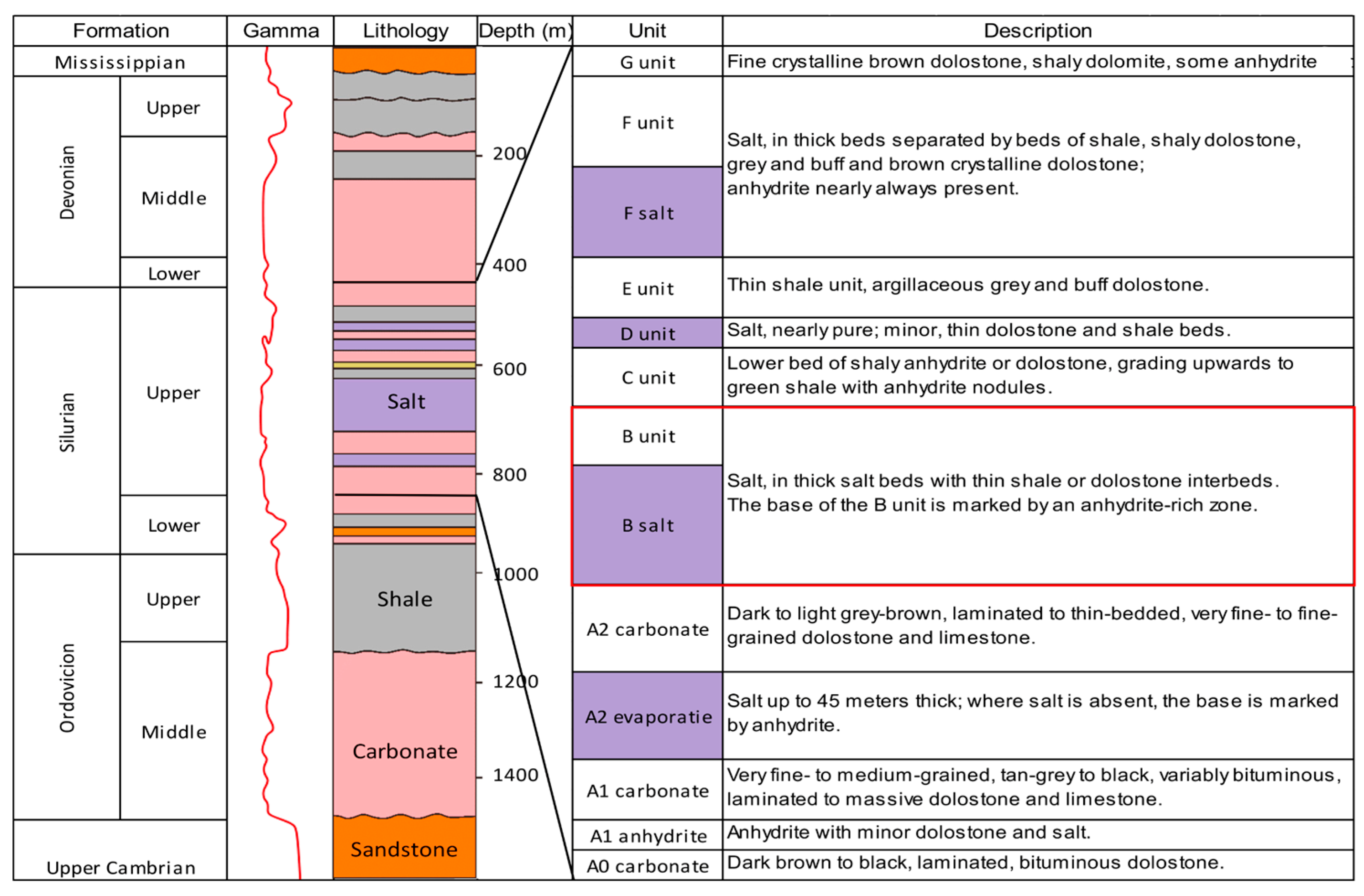
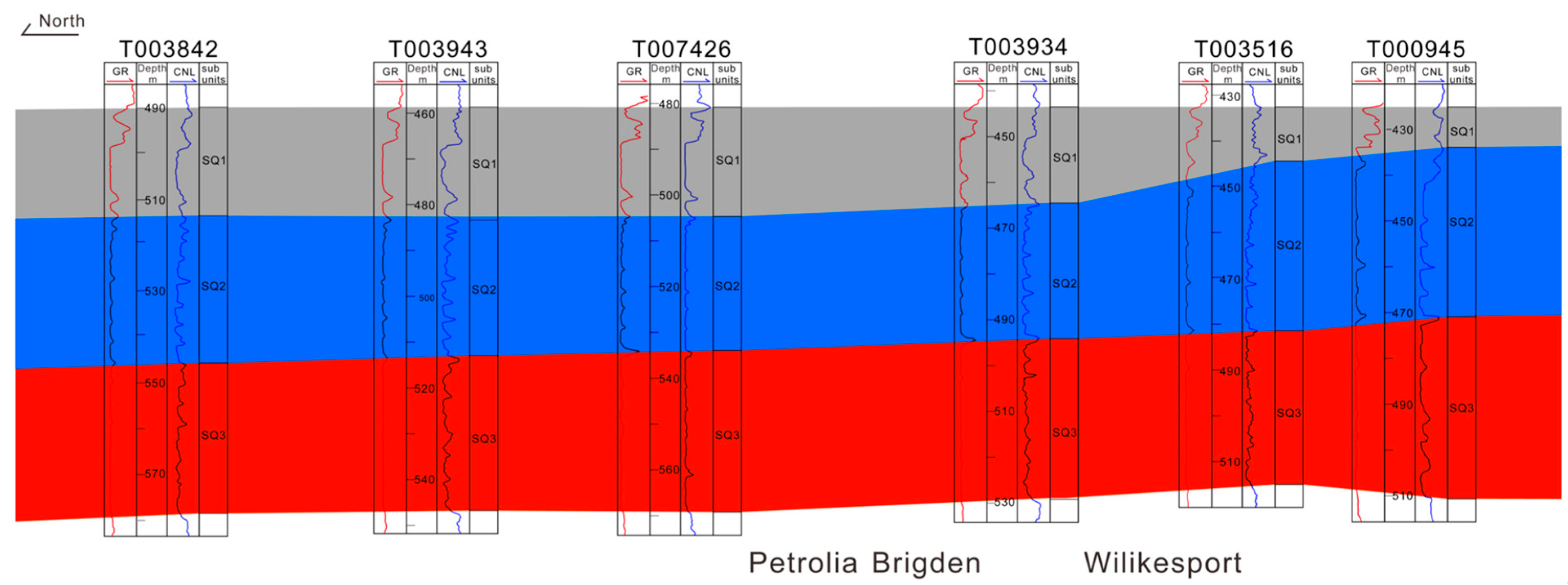
2. Geological Setting

The Michigan Basin, located in the southwestern area of southwestern Ontario, underlies the Salina Formation of the Silurian age. The Salina Formation can be systematically divided into seven units, labeled A through G, based on lithofacies characteristics. Among these, units F, D, B, and the lower part of A2 all contain halite deposits [29]. However, due to the vertical inconsistency of the rock layer properties, only unit B is considered a potential large-scale CAES construction site. The F unit contains various impurity components, including shale, dolomitic interlayers, and anhydrite, which pose obstacles to cavern construction and threaten overall stability. Though unit D and unit A2 contain pure salt rock mass, the space they can provide is insufficient for large-scale CAES, with unit D averaging a thickness of 12 m and unit A2 having a maximum salt layer thickness of 35 m [30]. The detailed lithology distribution of the Salina Formation is listed in Figure 1.

Based on the analysis of natural gamma (GR) and compensated neutron log (CNL) curves, two distinct sequence boundaries have been identified within the B unit. Accordingly, the unit is subdivided from top to bottom into three high-frequency sequence subunits: SQ1, SQ2, and SQ3. Specifically:

• The SQ1 subunit is characterized by high GR and CNL values, corresponding to interbedded halite and limestone;
• The SQ2 subunit consists of dark, laminated halite with pronounced fluctuations in the logging curves;
• The SQ3 subunit exhibits relatively stable and lower curve values, indicative of massive halite deposits.

Figure 2 illustrates the components of these subunits and around unit B, using data from wells F006864 and T003039 as examples [28]. Each subunit is distinguished by a different color.

The thicknesses of subunits SQ1, SQ2, and SQ3 in unit B generally range from 20 to 30 m, from 25 to 35 m, and from 30 to 40 m, respectively. SQ1 should be excluded from salt cavern construction due to its high limestone content. Although SQ2 contains shale sublayers, it is still considered for salt caverns to obtain maximum storage volume. Figure 3 illustrates the north–south spatial variation in the thickness of halite subunits within a representative area of the central Michigan Basin, specifically the Petrolia–Bridge–Wilkesport zone. In Figure 3, the thickness variation shows a relatively gentle and uniform distribution trend in the studied area. Therefore, the strata are assumed to be flat for the sake of model simplicity. The thicknesses of SQ2 and SQ3 are defined as 30 m and 35 m, respectively, both representing their average values and closely aligning with the geological conditions observed in the northern Petrolia region, as shown in Figure 3. Given the presence of randomly distributed shale layers in subunit SQ2, five equidistant shale layers, each 1 m thick, are incorporated into the model to better represent the heterogeneity of the bedded salt deposit. Subunit SQ3 is assumed to be pure salt based on the relatively stable trends with low GR and CNL values in the GR log of SQ3.

To conclude, the three-dimensional stratigraphic model measures 200 m × 200 m × 100 m and features a representative sequence structure: a 25 m-thick SQ1 limestone layer at the top, underlain by a 30 m-thick SQ2 halite layer containing five shale interbeds, which gradually transitions into a 35 m-thick SQ3 pure halite layer. The basal unit consists of a 3 m-thick anhydrite layer and a 7 m-thick limestone layer.

3. Constitutive Model

3.1. Elastoplastic Constitutive Model

The Drucker–Prager material model is widely used in geotechnical and petroleum engineering, particularly for analyzing rocks with significant plastic behavior and focusing on short-term processes such as borehole drilling and cavern excavation. It captures the frictional and cohesive characteristics of materials well and is easier to implement in finite element methods.

According to the conventional representation in rock mechanics, where compressive stress is considered negative, the yield criterion of the Drucker–Prager model can be expressed as follows [31]:

$$\mathrm{f}\left(\mathsf{\sigma }\right)=\sqrt{{\mathrm{J}}_2}+\mathsf{\alpha }{\mathrm{I}}_1-\mathrm{k}=0$$

(1)

where ${\mathrm{J}}_2$ is the second invariant of the stress deviator tensor, and ${\mathrm{I}}_1$ is the first invariant of the stress tensor.

${\mathrm{J}}_2$ and ${\mathrm{I}}_1$ are defined as follows:

$${\mathrm{J}}_2={\displaystyle \frac{1}{6}}[{({\mathsf{\sigma }}_1-{\mathsf{\sigma }}_2)}^2+{({\mathsf{\sigma }}_2-{\mathsf{\sigma }}_3)}^2+{({\mathsf{\sigma }}_1-{\mathsf{\sigma }}_3)}^2]$$

(2)

$${\mathrm{I}}_1={\mathsf{\sigma }}_1+{\mathsf{\sigma }}_2+{\mathsf{\sigma }}_3$$

(3)

${\mathsf{\sigma }}_1$, ${\mathsf{\sigma }}_2$, and ${\mathsf{\sigma }}_3$ are the principle effective stresses, and α and k are material constants connected to the material’s cohesion and friction angle. The correlations are as follows:

$$\mathsf{\alpha }={\displaystyle \frac{2\sin \mathsf{\phi }}{\sqrt{3}(3-\sin \mathsf{\phi })}}$$

(4)

$$\mathrm{k}={\displaystyle \frac{6\mathrm{c}\cos \mathsf{\phi }}{\sqrt{3}(3-\sin \mathsf{\phi })}}$$

(5)

where φ is the internal friction angle of the rock, and c is the cohesion.

3.2. Creep Constitutive Model

In this study, the rheological behavior of halite is characterized using the Norton creep equation, which is expressed as follows [32]:

$$\dot{\mathsf{\epsilon }}\left(\mathrm{t}\right)=\mathrm{A}{\mathrm{q}}^{\mathrm{n}}$$

(6)

where A and q are rock creep variables, and q is a variable connected to stress. The correlation between q and stress is expressed as follows:

$$\mathrm{q}=\sqrt{3{\mathrm{J}}_2}$$

(7)

3.3. Evaluation Model of Tightness

To simulate the leakage of compressed air during the long-term injection–extraction cycles, the Darcy’s law module is applied. The basic equations are as follows:

$${\displaystyle \frac{\partial }{\partial \mathrm{t}}}\left({\mathsf{ϵ}}_{\mathrm{p}}\mathsf{\rho }\right)+\nabla \left(\mathsf{\rho }\mathrm{u}\right)={\mathrm{Q}}_{\mathrm{m}}$$

(8)

$$\mathrm{u}=-{\displaystyle \frac{\mathsf{\kappa }}{\mathsf{\mu }}}(\nabla \mathrm{p}-\mathsf{\rho }\mathrm{g})$$

(9)

where ${\mathsf{ϵ}}_{\mathrm{p}}$ is the porosity of the surrounding rock, $\mathsf{\rho }$ is the density of the air, ${\mathrm{Q}}_{\mathrm{m}}$ is the mass resources, κ is the permeability of the surrounding rock, μ is the dynamic viscosity, p is the pressure, and u is the permeation velocity. The low pore space dimension and the low permeability of the condensed salt rock mass will significantly decrease the Reynolds numbers; thus it is safe to consider that the air flow in the surrounding salt rock conforms to Darcy’s law. The equation takes gravity into consideration and assumes the hosting rock to be isotropic.

Considering the porous rock background, the equation can be written as follows:

$${\mathsf{\rho }\mathrm{s}}_{\mathrm{p}}{\displaystyle \frac{\partial \mathsf{\rho }}{\partial \mathrm{t}}}+\nabla \left(\mathsf{\rho }\mathrm{u}\right)={\mathrm{Q}}_{\mathrm{m}}$$

(10)

$${\mathrm{s}}_{\mathrm{p}}={\mathsf{ϵ}}_{\mathrm{p}}{\mathsf{\chi }}_{\mathrm{f}}+(1-{\mathsf{ϵ}}_{\mathrm{p}}){\mathsf{\chi }}_{\mathrm{p}}$$

(11)

where ${\mathsf{\chi }}_{\mathrm{f}}$ is the compressibility of the air, and ${\mathsf{\chi }}_{\mathrm{p}}$ is the compressibility of the hosting rock.

4. Numerical Model

In this study, a numerical model was developed using the COMSOL Multiphysics 6.2 simulation platform, based on actual well-logging data from the B unit. The model geometry is defined as 200 m in length, 200 m in width, and 100 m in height, with the top surface buried at a depth of 475 m. Based on computational analysis, the average density of the overlying strata is assumed to be 2300 kg/m³. The detailed mechanical properties of the rock mass are listed in

Table 1. Basic rock properties for rock layers.

Lithology	Young’s Modulus (GPa)	Poisson’s Ratio	Density (kg/m3)	Cohesion (MPa)	Angle of Internal Friction (deg)
Shale	25	0.35	2500	1.5	25
Salt	2.26	0.28	2200	5.76	31.6
Anhydrite	12.9	0.22	3000	3.2	35
Limestone	20	0.23	2700	15.9	36

.

4.1. Cavern Design

Salt caverns are typically constructed through leaching owing to the water-soluble property of salt. In the leaching process, water is pumped through the well and semi brine is collected, which can be further processed for salt production. The leaching method has been refined over the years, allowing for better control of the salt cavern shape by adjusting the leaching path and operating parameters to achieve the desired geometry [33]. For example, two basic leaching strategies, direct and indirect leaching, can lead to different cavern shapes. In direct leaching, freshwater is injected through a central tubing to the bottom of the cavern, where it dissolves the salt rock. The resulting brine is then extracted through the outer casing. This method typically results in the formation of a cylindrical cavern. In contrast, the indirect or reverse leaching method introduces freshwater from the top through the outer casing and dissolves the salt rock at the bottom of the cavern. The resulting brine is then withdrawn through the central tubing. This method tends to form a pear-shaped cavern with an enlarged top [34]. Both leaching methods will leave a layer of insoluble sediment at the cavern bottom. A schematic depicting both methods is shown in Figure 4. However, indirect leaching is not recommended for designing salt caverns intended for energy storage, as the resulting cone-shaped cavern significantly reduces the utilization rate of underground space. Moreover, leaching program parameters, such as the injection rate and water volume, play a crucial role in controlling the resulting cavern shape. By adjusting these parameters, an elliptical-shaped salt cavern can be achieved, helping to avoid sharp corners and mitigate stress concentrations [33]. However, achieving perfectly shaped caverns is challenging even with intentional controls, as layers containing insoluble materials can cause irregularities in the cavern shape. These irregularities often manifest as bevels, ledges, “necks”, or “waists” in bedded salt deposits with less soluble interlayers [35], but adjustments in leaching methods and leaching program parameters can help reduce such irregularities. Moreover, since these irregularities are difficult to predict prior to leaching, cavern shapes are often assumed to be regular in preliminary studies.

In addition to cavern shape, the geometric parameters also need to be considered carefully when designing a salt cavern for energy storage. In bedded salt deposits, a minimum height-to-diameter ratio of 0.5 is required to maintain geomechanical stability. It is recommended that the hanging wall have a minimum thickness of 75% of the cavern diameter, while the footwall thickness should be at least 20% of the cavern diameter [36]. Additionally, some studies suggest that for thin salt layers, the hanging wall should be no less than 20 m thick, with a minimum footwall thickness of 10 m [37,38].

In this study, two basic cavern shapes were adopted for simulation: cylinder and ellipsoid. An upside-down cone-shaped cavern was neglected due to its smaller volume. Each cavern was modeled with a fixed height of 35 m, ensuring a recommended 20 m-thick hanging wall and a 10 m-thick footwall to maintain basic stability. For each shape, five diameters were selected: 17.5 m, 35 m, 52.5 m, 70 m, and 87.5 m, corresponding to diameter-to-height ratios of 0.5, 1, 1.5, and 2. The models assume that 15% of insoluble sediment remains at the bottom of the cavern after leaching. Calculations for the height of sediments for each shape of cavern are as follows:

• Cylinder

$$\mathsf{\pi }{\mathrm{r}}^2\mathrm{h}=0.15\mathsf{\pi }{\mathrm{r}}^2\mathrm{H}$$

(12)

$$\mathrm{h}=0.15\mathrm{H}=5.25 \mathrm{m}$$

(13)

2.

Ellipsoid

To optimize the utilization of underground space, the ellipsoid is designed with a circular cross-section. It is assumed that the ratio between the ellipsoid’s horizontal parameter and its height is denoted as a. Accordingly, the ellipsoid equation can be expressed as:

$${\displaystyle \frac{{\mathrm{x}}^2}{{{\mathrm{a}}^2\mathrm{H}}^2}}+{\displaystyle \frac{{\mathrm{y}}^2}{{{\mathrm{a}}^2\mathrm{H}}^2}}+{\displaystyle \frac{{\mathrm{z}}^2}{{\mathrm{H}}^2}}=1$$

(14)

Setting the cross-section at half of the height of the ellipsoid as the coordinate system plane, the following is obtained:

$${\int }_{-\frac{\mathrm{H}}{2}}^{-(\frac{\mathrm{H}}{2}-\mathrm{h})}\mathsf{\pi }(1-{\displaystyle \frac{{\mathrm{z}}^2}{{\mathrm{H}}^2}}){\mathrm{a}}^2{\mathrm{H}}^2\mathrm{d}\mathrm{z}=0.15{\displaystyle \frac{4}{3}}\mathsf{\pi }{\mathrm{a}}^2{{\displaystyle \frac{\mathrm{H}}{8}}}^3$$

(15)

For H = 35 m, the equation leads to:

$$\mathrm{h}=8.55 \mathrm{m}$$

(16)

4.2. Operating Pressure Design and Leakage Evaluation

CAES systems store energy by compressing air during periods of low electricity demand and releasing it to generate electricity during peak demand. During storage, compressed air is injected into salt caverns and withdrawn when needed. Ideally, the maximum internal pressure should be as high as possible, while the minimum internal pressure should be as low as possible to maximize storage capacity. However, operating pressures must be carefully maintained within safe limits, as the operation of huge storage causes cyclic loading posed on the cavern wall, creating great engineering disturbances in geological bodies of salt rock and dramatic changes the stress state and loading condition. Salt rocks exhibit pronounced plastic deformation and creep behavior; therefore, salt caverns will undergo long-term deformation that potentially leads to inevitable damage, including cavern collapse and energy leakage, if the operating pressure is too high [39].

When designing the propriate operating pressure, another essential step is evaluating the tightness of the system with the chosen operating pressure, as this parameter is the key driving force for energy leakage. Compressed air stored in the cavern will inevitably dissipate into the surrounding rock mass, and higher operating pressures will accelerate this process. Moreover, excessive operating pressure can lead to fractures, further exacerbating energy leakage and compromising the system’s integrity [40]. Although salt rock provides a naturally sealed storage space, the interlayers can serve as potential leakage pathways, and the changing stress field may intensify this leakage. Therefore, tightness evaluation is essential to ensure that the operating pressure is not excessively high.

Previous studies suggest that the gas pressure inside the cavern should be maintained between 30% and 85% of the vertical pressure at the cavern top to ensure stability [41,42]. In this study, potential operating pressures of 0.3, 0.4, 0.5, 0.6, 0.7, and 0.8 times the vertical stress are evaluated. Stationary simulations are first conducted using these operating pressures, and the resulting deformations are analyzed to assess their impact on cavern stability. Based on the findings, the operating pressures with the least influence on overall stability are selected for further analysis. A time-dependent simulation is then performed, incorporating the creep behavior and plastic deformation of salt rock to evaluate the selected pressure range and optimize working pressure during operation. The simulation spans 10 years to estimate total plastic deformation and creep deformation distributions, and the injection production frequency is set to be four times per year, providing insights into the long-term performance and safety of the storage system.

5. Modeling Results

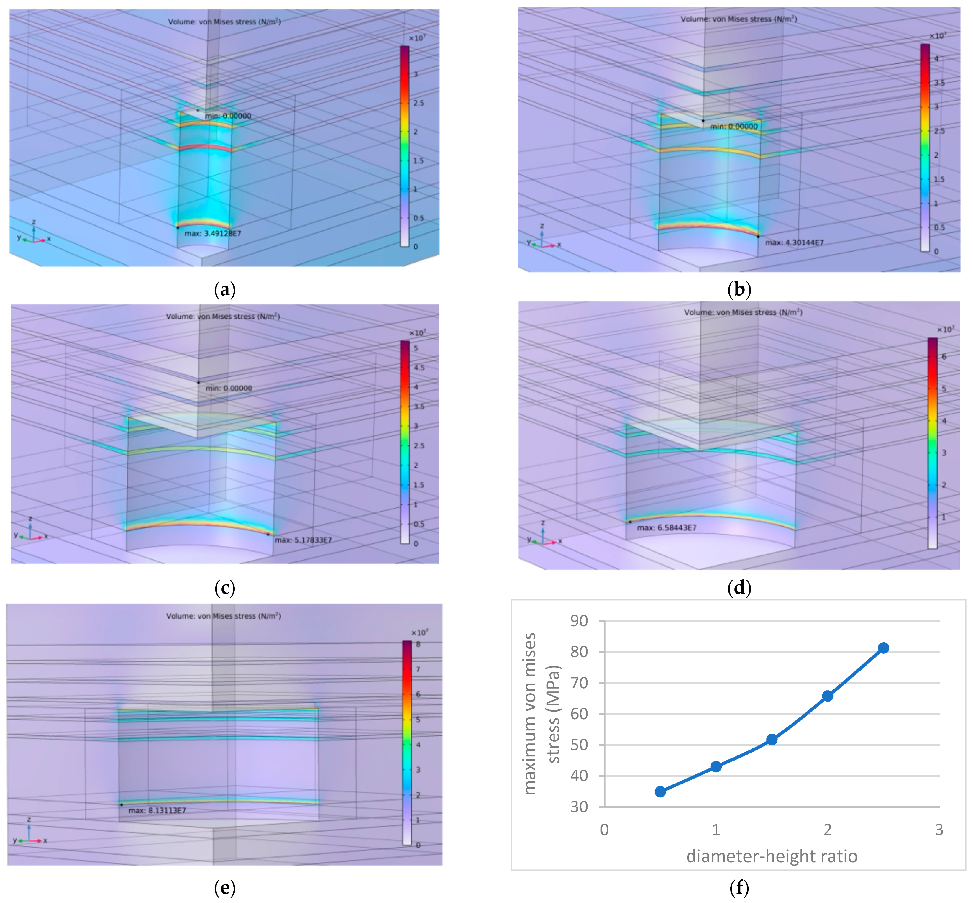
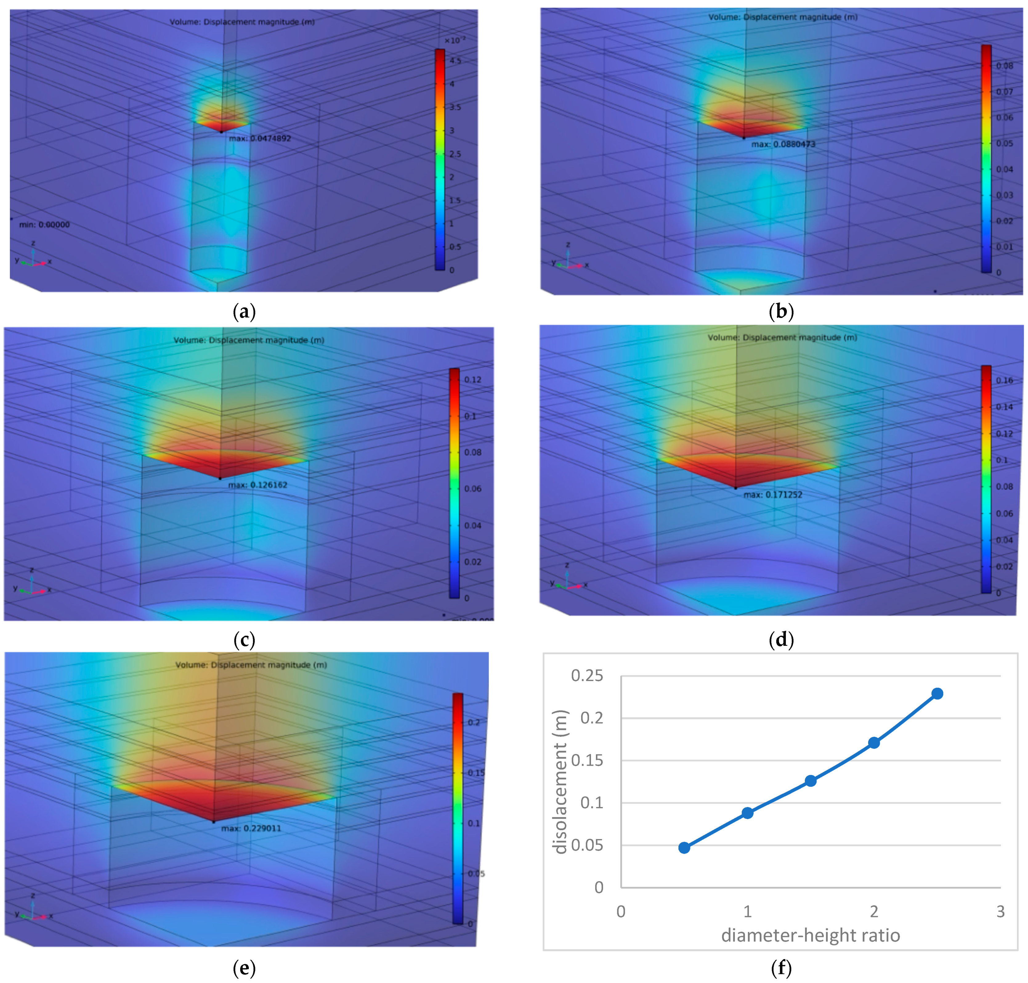
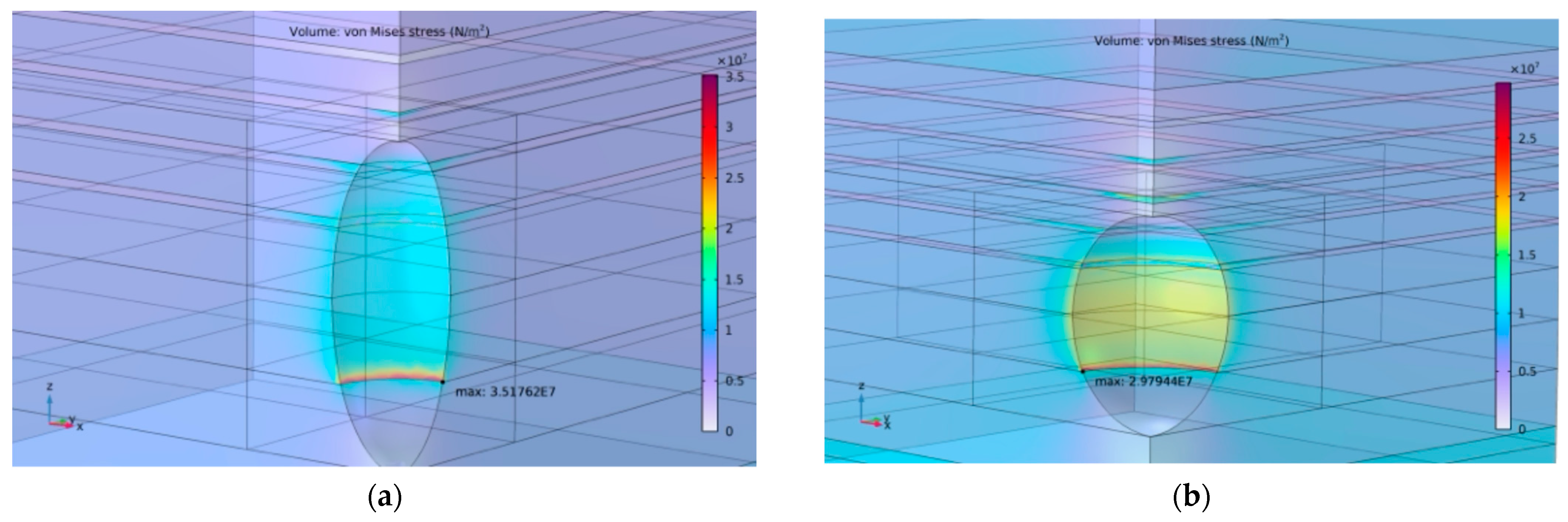
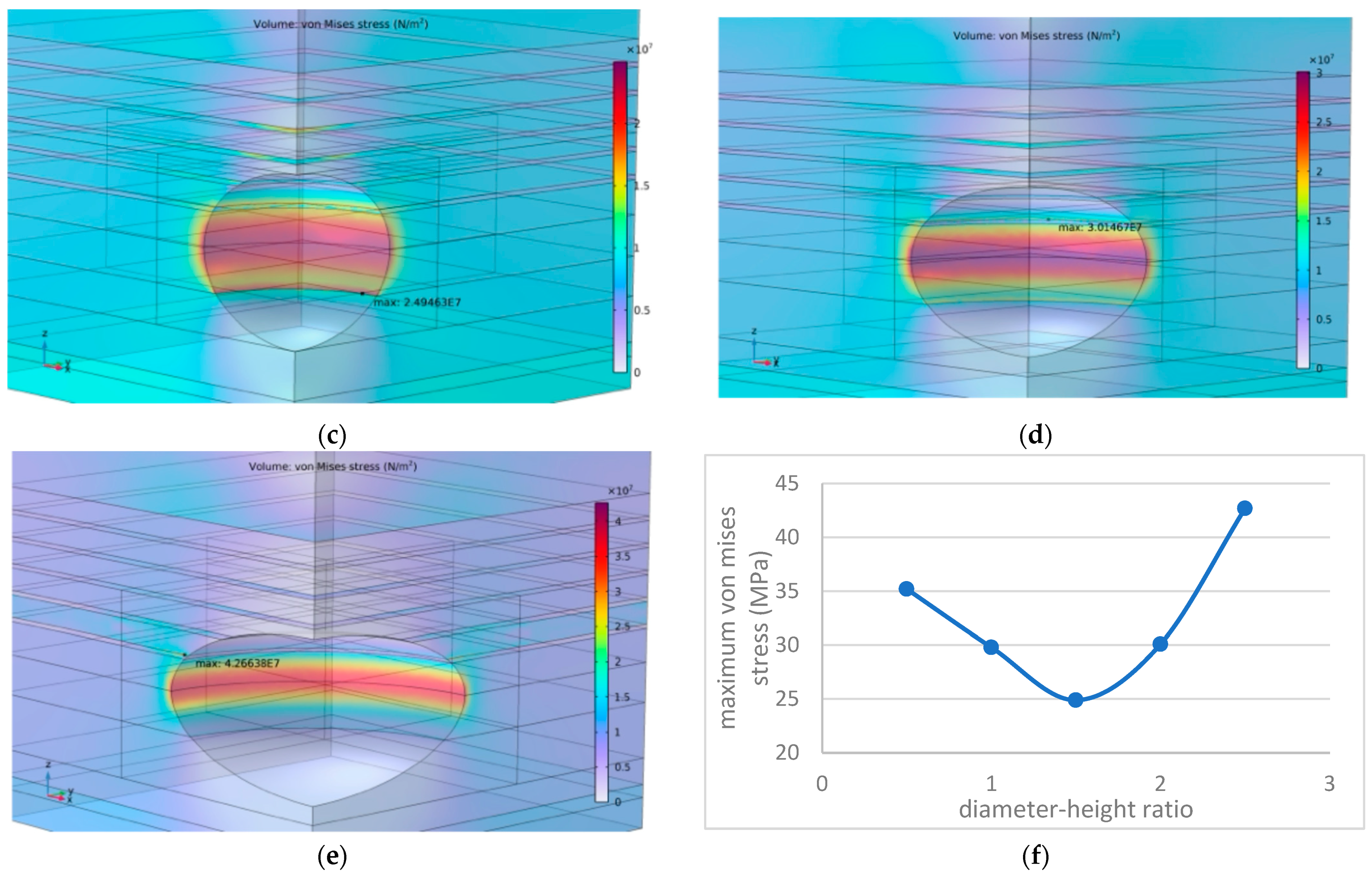
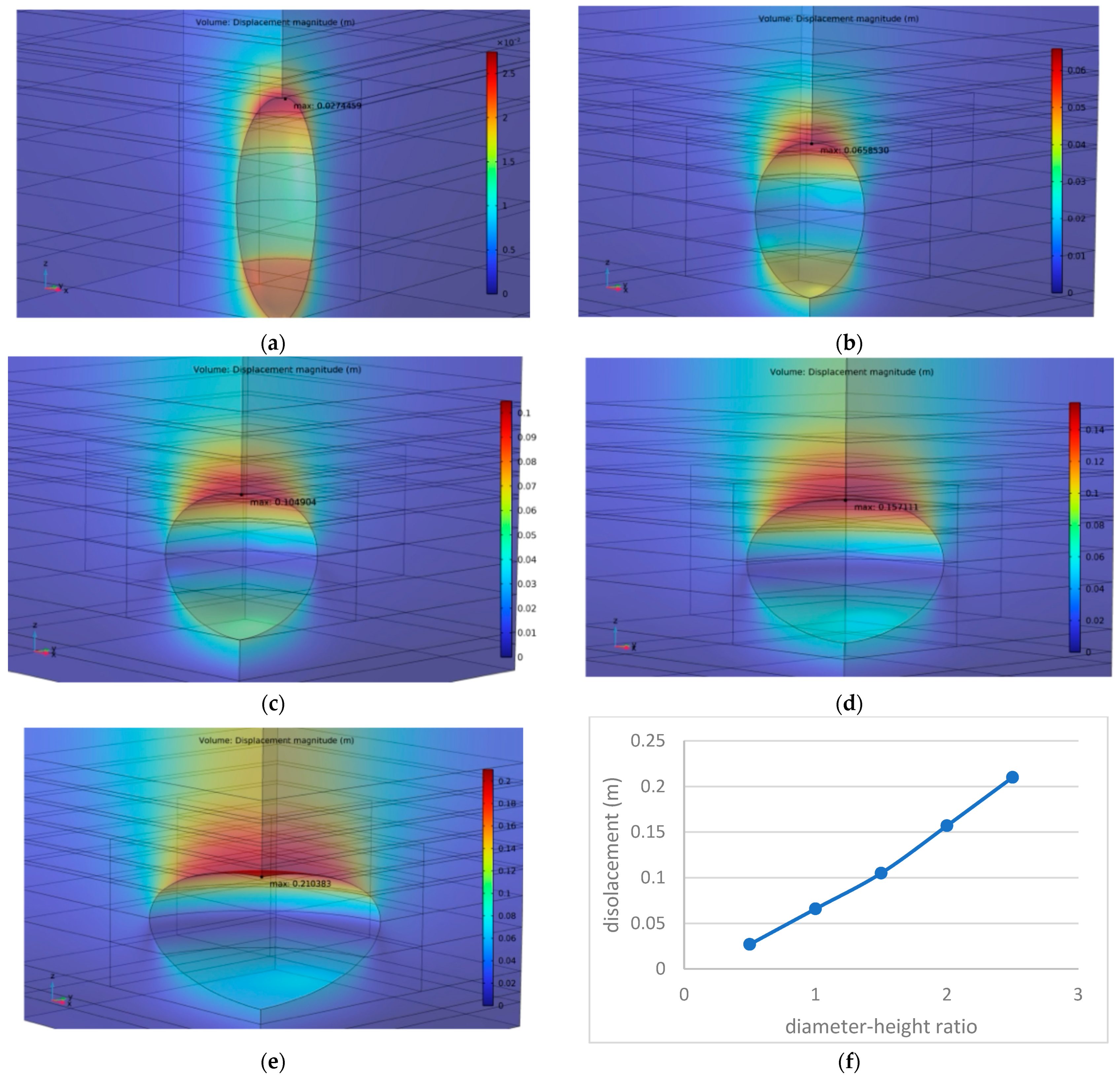
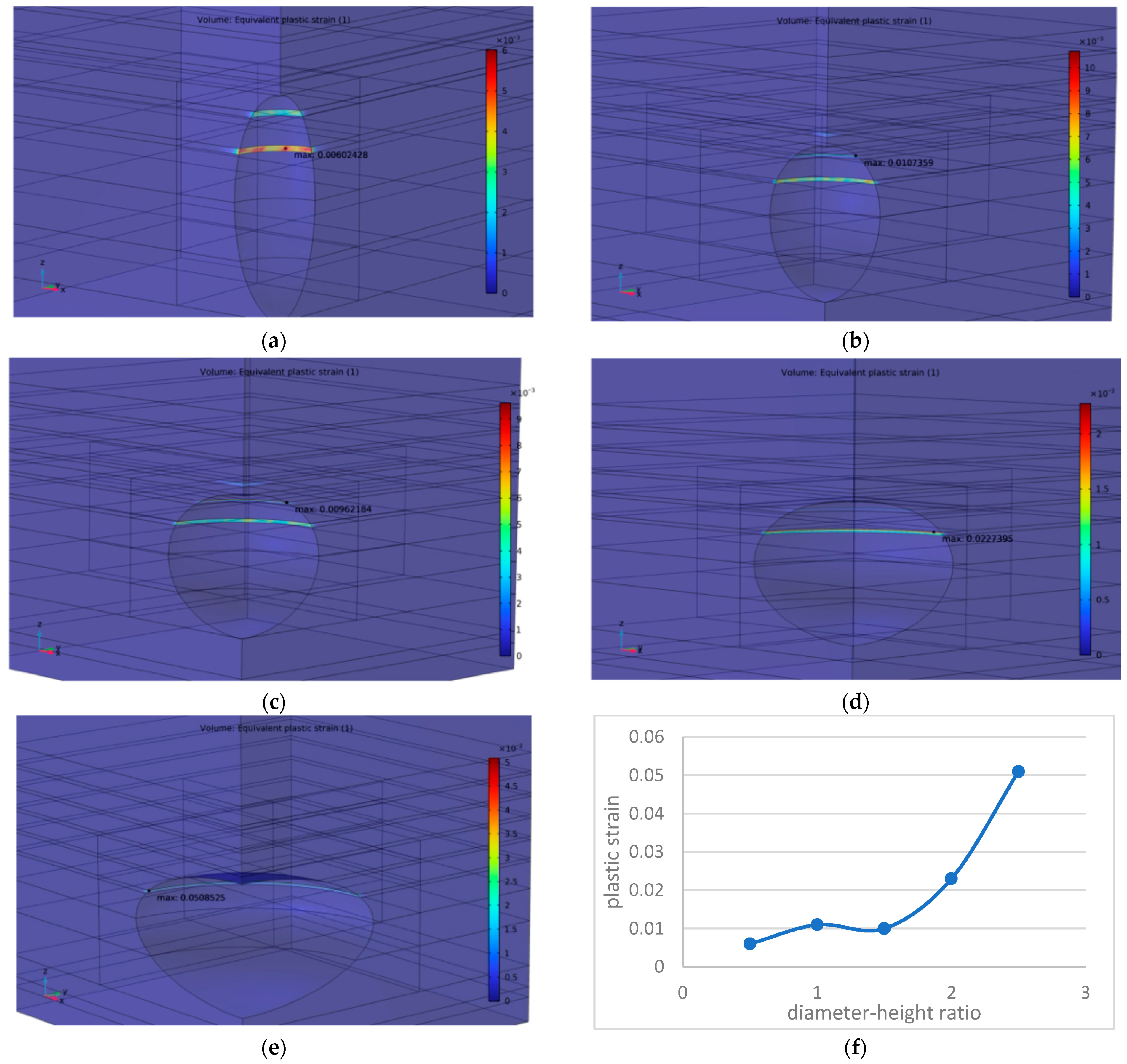
5.1. Cavern Shape and Parameter Optimization

To investigate the impact of cavern shapes on the overall stability of the CAES system and determine the optimal shape, the von Mises stress distribution and displacement contour maps, as well as plastic deformation development for each cavern shape after leaching, were analyzed as follows:

• Cylinder

Cylinder-shaped caverns are set with diameters of 0.5, 1, 1.5, 2, and 2.5 times their height. After excavation, the von Mises stress fields are determined, as shown in Figure 5.

For salt caverns with varying diameters, the von Mises stress is consistently concentrated in the embedded shale layers surrounding the caverns and at the edges of the top and bottom of cylindrical-shaped caverns. The sharp corners of the cylindrical caverns introduce stress concentrations, resulting in higher von Mises stress levels and making them more susceptible to potential hazards. The maximum von Mises stress is generally located at the edge of the cavern roof, along both the x-axis and y-axis directions, aligning with the direction of the horizontal stresses. The concentration of von Mises stress in the embedded shale layers is attributed to their weaker geomechanical properties, making these areas another potential source of concern. However, stress concentration in the shale layers is less pronounced compared to the cavern roof, as the von Mises stress increases more significantly at the edge of the upper roof with the growth in cavern diameters.

According to the maximum von Mises stress curve, as the height-to-diameter ratio increases, the von Mises stress shows an initially linear increase followed by an accelerated rise, with a turning point occurring at a ratio of 1.5. Beyond this critical value, stress concentration in the cavern bottom region becomes significantly more pronounced, suggesting that the salt rock in this area is approaching the onset of plastic yielding.

Displacement contour plots of different caverns are shown in Figure 6.

Figure 6 illustrates that after leaching, the cavern roof exhibits a significant tendency of deformation, bending downward. This settlement trend extends into the overlying rock layers but gradually diminishes with distance. Other parts of the cavern, including the walls and floor, also show inward deformation tendencies. However, this inward extrusion weakens at the junctions between different rock layers, resulting in less deformation in the shale layers compared to the salt rock mass, even though the difference is minor and has little influence on the overall stability of the salt caverns. Notably, inward deformation is more pronounced in caverns with smaller diameters. While displacements around the salt cavern generally increase with cavern diameter, the rate of deformation growth is most significant at the cavern roof.

The biggest displacement occurs at the central part of the cavern roof for caverns with all different diameters. With the increase in diameter-to-height ratio, the displacement grows linearly to 0.229 m when the ratio reaches 2.5. This linear growth indicates that the salt rock at the roof center remains within the elastic range. However, the overall stability of the cavern is not guaranteed, as excessive displacement can pose potential risks to the system.

To better analyze the plastic development of the cavern wall, the plastic strain clouds are plotted, as presented in Figure 7.

According to the plastic strain contours for caverns with varying diameters, the plastic strain in salt caverns of different sizes is primarily concentrated in four critical regions: the salt rock layer near the sidewalls of the cavern roof, the two embedded shale layers, and the salt rock zone near the sidewalls of the cavern floor. In caverns with smaller diameters, plastic deformation in all four areas remains minor, with small, localized plastic zones. As the diameter-to-height ratio increases, deformation in all four areas develops further, while areas in the salt rock near the cavern sidewalls close to the floor develop the most significantly. This pronounced deformation is influenced not only by the higher stress field at greater depths but also by stress concentrations at the cavern corners, with the latter playing the most critical role in enhancing plastic deformation. This is further evidenced by the plastic deformation in the salt rock near the cavern sidewalls close to the roof. While the shale interlayers also exhibit plastic deformation trends, they are less significant compared to other areas. Nonetheless, they should not be overlooked, as deformation in these layers increases rapidly when the diameter-to-height ratio reaches 2.

The maximum plastic strain varies with cavern diameter, but predominant deformation occurs in the salt rock zone adjacent to the sidewalls of the cavern roof. It generally increases linearly with the diameter-to-height ratio until the ratio reaches 2, beyond which a significant acceleration is observed, indicating the stability limit is being approached.

In summary, while considering both the stability and the capability, the best diameter may be set to 1.5 to 2 times the height in unit B when the cavern shape is determined to be a cylinder.

• Ellipsoid

For an ellipsoid shape, the diameters of the cross-section circle at the middle of the cavern are seen as the cavern diameter, and they are set to be 0.5, 1, 1.5, 2, and 2.5 times its height. After excavation, the von Mises stress fields are determined, as shown in Figure 8.

The von Mises stress cloud plots reveal that the stress concentration in ellipsoidal salt caverns exhibits a distinct spatial distribution pattern. Overall, two dominant concentration zones are observed: the edge of the cavern roof and the midsection of the sidewalls. Before the diameter-to-height ratio reaches around 1.5, the stress concentration is primarily confined to the cavern wall near the roof edge, indicating that the stress concentration induced by the sediment layer is the prominent factor. When the ratio reaches 1.5, the stress concentration can be found in both regions. As the ratio continues to increase, the concentration shifts further toward the central region. The von Mises stress at the edge near the top of the sediment layer decreases as the diameter increases, due to the widening angle between the sediment and the cavern wall. Consequently, the stress difference between this area and the surrounding salt cavern wall diminishes as stress concentration along the central cavern wall becomes increasingly prominent, with this difference disappearing when the diameter-to-height ratio reaches 2.5. Unlike the salt rock around the sediment surface, the stress concentration in the middle part of the cavern keeps growing as the cavern shape flattens with increasing diameter. Therefore, an initial drop trend in the maximum von Mises stress can be found as the stress in the middle part of the cavern fails to exceed that in the salt around sediment surface, and it begins to increase dramatically after the diameter-to-height ratio reaches 1.5 as the stress concentration in the middle cavern begins to show its prominence.

Despite the rapid growth in the stress concentration in the middle part of cavern, the maximum von Mises stress is found in the interlayers after the diameter-to-height ratio reaches 2. This is because as the diameter increases, the angle between the cavern wall and the interlayer becomes sharp, aggravating the stress concentration. Before that, the maximum von Mises stress is found in the cavern wall around the sediment top surface. Compared with the cylinder-shaped cavern with same diameter, the maximum von Mises stress is much lower, especially at the diameter-to-height ratio of 1.5. However, though bearing a much lower von Mises stress, the narrow angle between the interlayer and the cavern wall makes the stress concentration significantly prominent, posing a potential threaten to the cavern stability. Moreover, the insoluble contents of the interlayers make the cavern shape hard to control; thus, such a stress concentration may be hard to predict in the simulation period.

Besides the von Mises stress contribution, the displacement contour of each cavern after leaching is determined, as shown in Figure 9.

The displacement distribution exhibits a pattern similar to that of cylindrical-shaped caverns: the cavern roof bends downward, while the floor protrudes upward. The most significant displacement occurs at the center of the cavern roof. However, compared to cylindrical-shaped caverns, the floor’s protrusion tendency is more pronounced, and the deformation in the interlayers tends to be more uniform with the surrounding salt rock. Additionally, the maximum displacement is slightly smaller than that of a cylindrical-shaped cavern with the same diameter and increases linearly with the diameter.

Figure 10 illustrates the plastic strain distribution.

Unlike cylindrical-shaped caverns, plastic deformation in ellipsoid-shaped caverns is mainly confined to the bedded shale interlayers. Although the sediment layers introduce stress concentration and significant displacement is observed at the cavern floor, the ellipsoid shape effectively mitigates plastic deformation in the surrounding salt rock. However, plastic deformation within the interlayers remains prominent, with the maximum plastic strain being significantly higher than that in cylindrical-shaped caverns of the same diameter. This elevated plastic strain makes the interlayers more susceptible to potential hazards such as fracturing. As the diameter-to-height ratio increases, the plastic strain generally rises, except for caverns with a ratio of 1.5, where a temporary reduction is observed. Beyond a ratio of 1.5, plastic deformation intensifies dramatically, indicating an increasing threat to overall cavern stability.

Based on the above findings, this study identifies the cylindrical salt cavern with a height-to-diameter ratio of 1.5 as the most suitable structural configuration for CAES. Although ellipsoid-shaped caverns exhibit a significantly lower stress field due to the reduced stress concentration, their shape is challenging to control during the leaching process. The presence of insoluble materials in the interlayers further complicates shape predictability around these zones. Additionally, ellipsoid-shaped caverns experience much higher plastic strain compared to cylinder-shaped caverns. In contrast, a cylindrical cavern offers better structural stability and a larger storage capacity for the same diameter, making it the preferred choice for practical implementation.

5.2. Operating Pressure Optimization

5.2.1. Stational Analysis for Initial Selection of Operating Pressure

Through a series of scenarios analyzing 0.3 to 0.8 times the vertical stress, the static analysis results reveal a consistent pattern in stress distribution. To maintain conciseness, this study presents the typical distribution characteristics under 0.4, 0.6, and 0.8 times the vertical stress, as these cases effectively capture the mechanical response trends across the entire pressure range. Figure 11 presents the displacement contours.

Shown in the displacement contours for different operating pressures posed on the cavern wall, the cavern roof exhibits predominant downward deformation, while the floor shows upward extrusion; both deteriorate with the increasing operating pressure. This occurs because the operating pressure tends to make the cavern expand, countering with the shrinking tendency of the cavern brought on by the highly compressive geological stress field. This is further demonstrated by the displacement development along the sidewall as the operating pressure increases. For caverns subjected to low operating pressure, the sidewalls exhibit a tendency for inward extrusion, though the displacement values remain minimal. As shown in the figure, when the operating pressure ratio is 0.4, most of the sidewall displacement is less than 0.01 m, with substantial areas displaying no displacement, which significantly enhances the stability of the cavern sidewall. As the operating pressure increases and exceeds the far-field stress acting on the sidewall, the salt rock displays an outward bending tendency. As shown in the figure, at an operating pressure of 0.8 times the vertical stress, the salt rock mass on the sidewall bends outward, while the shale interlayers experience a relatively minor deformation, forming a supporting function. Consequently, the maximum displacement of the sidewall salt rock is found in the middle section, posing a potential threaten of cavern failure.

Before the operating pressure reaches 0.7 times the vertical stress, the maximum displacement decreases steadily as the operating pressure increases. However, when the operating pressure reaches 0.8 times the vertical stress, the location of maximum displacement shifts from the central roof to the middle section of the sidewall. This indicates that the influence of operating pressure surpasses the compressive geological field somewhere between 0.7 and 0.8 times the vertical stress, potentially compromising the overall stability of the salt cavern.

The distribution of von Mises stress and plastic strain is shown in Figure 12.

Figure 12 shows that the von Mises stress consistently concentrates at both the upper and the lower edges of the salt cavern, regardless of the operating pressure, highlighting the predominant influence of the cavern’s sharp corners. Although the shale interlayers experience relatively minor deformation according to Figure 11, their von Mises stress increases more rapidly than that of the surrounding salt rock along the sidewalls. According to Figure 12, the von Mises stress is lower than that in the surrounding salt rock at an operating pressure of 0.4 times the vertical stress, while it surpasses that of the salt rock when the operating pressure ratio reaches 0.6, with the difference becoming significantly more pronounced at a ratio of 0.8. The high-stress field confined in the interlayers will inevitably damage the shale integrity, compromising the overall stability.

Despite the rapid increase in stress within the interlayers, the maximum von Mises stress across all cases is still observed at the cavern’s bottom edge. With the increase in the operating pressure, the maximum von Mises stress decreases, with the rate of decline slowing as the growing operating pressure counteracts the compressive geological field. The declining trend in stress plateaus between operating pressure ratios of 0.6 and 0.7, as the maximum von Mises stress values are nearly identical in these two cases. Beyond this point, the maximum von Mises stress begins to increase, indicating that the expanding force brought on by the operating pressure surpasses the confining effect of the stress field. Considering the cyclic loading demand of the CAES system, such a turning point should not be surpassed, as the compaction-to-expansion transform will harm the salt rock integrity significantly.

Considering everything discussed above, the minimum operating pressure is recommended to be 0.4 times the vertical stress, and the maximum operating stress is recommended to be around 0.7 times the vertical stress.

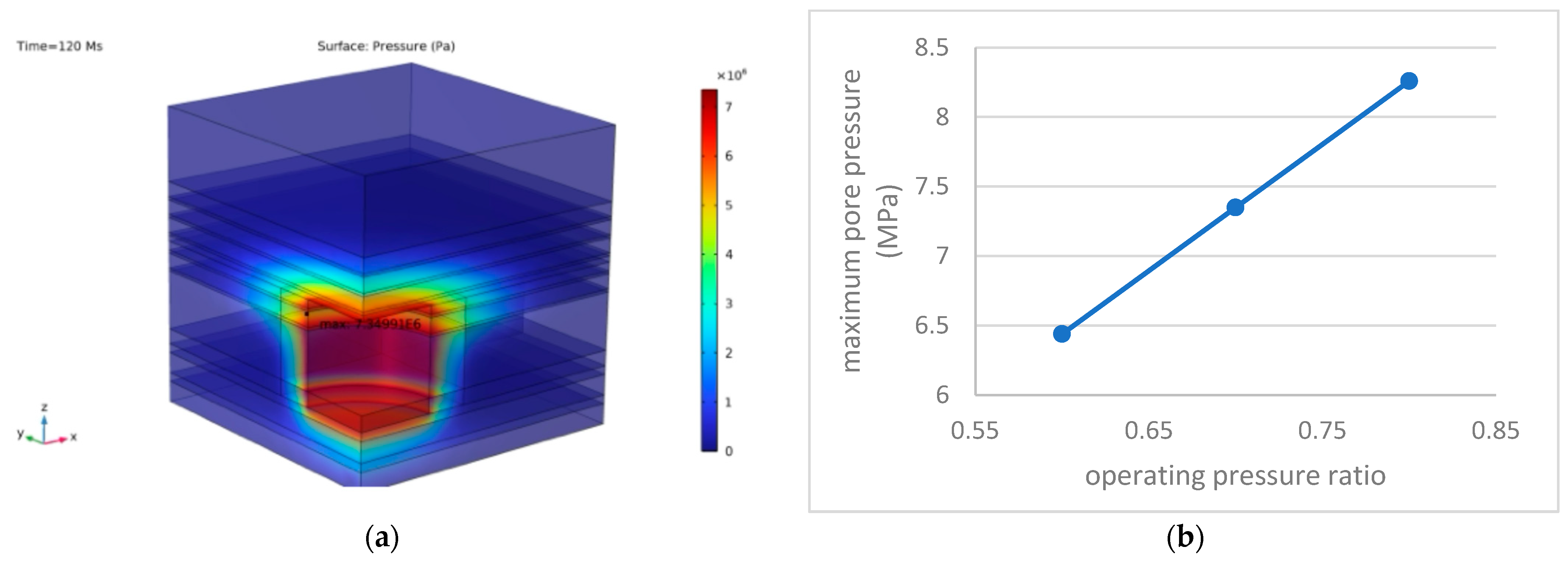
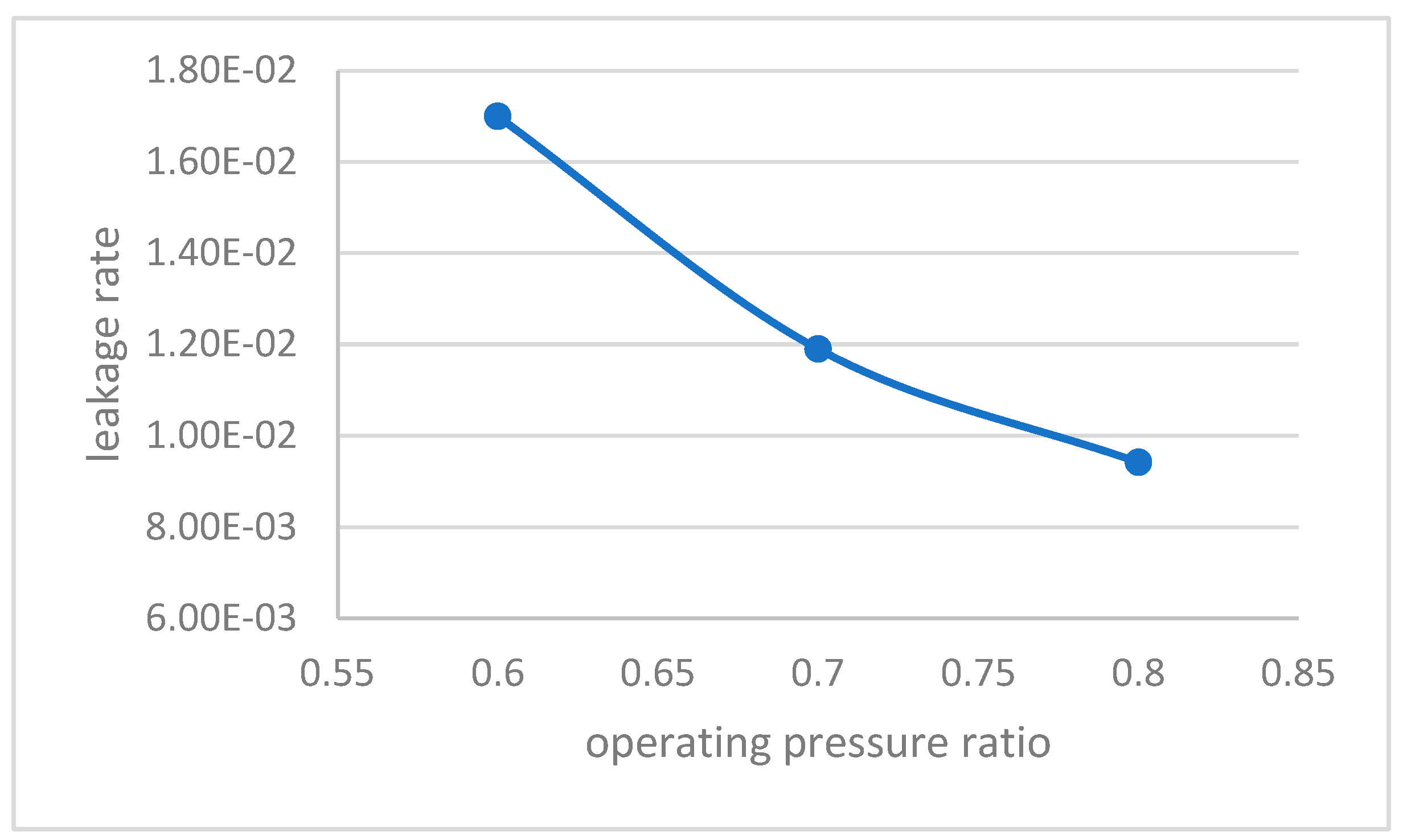
5.2.2. Tightness Evaluation

In this simulation, the fixed minimum operating pressure is set to be 0.4 times the vertical stress, as mentioned above, with 0.6, 0.7, and 0.8 times the vertical stress selected to be the potential maximum operating pressure for simulation. The simulation period is set to be 10 years, with four injection–withdrawal cycles per year, and the total gas leakage rate of each case is compared. Relevant rock properties are shown in

Table 2. Percolation properties for rock layers.

Lithology	Permeability (m2)	Porosity	Compressibility (Pa−1)	Diffusion Coefficient (m2/s)
Shale	1 × 10−19	0.07	3.6 × 10−11	1 × 10−8
Salt	1 × 10−21	0.01	5.84 ×10−10	1 × 10−9
Anhydrite	1 × 10−19	0.04	1.3 × 10−10	1 × 10−8
Limestone	1 × 10−18	0.01	1 × 10−10	1 × 10−8

.

The initial pore pressure around the cavern is set to be 0, as the rock mass is assumed to be completely dry and fully compressed under high-pressure conditions. During the injection–production cycle, the stored air dissipates into the surrounding rock mass, with a portion becoming trapped in the pore throats, resulting in an increase in pore pressure. Therefore, the pore pressure distribution after the simulation effectively represents the leakage pattern. It is noteworthy that though leakage will also occur in the injection and extraction wells, such leakage can be neglected due to the small volume of the well compared to the salt rock deposit. Taking the maximum operating pressure of 0.7 times the vertical stress as an example, Figure 13 illustrates the resulting pore pressure distribution.

According to Figure 13, compressed air dissipates into the surrounding rock from all sides of the cavern, with the primary seepage pathway occurring through the embedded shale layers. With the rock property changing with the pore pressure induced, leaked air is trapped in the surrounding rock mass and accumulates. The rock mass near the cavern wall exhibits higher pore pressure levels, which decline rapidly with increasing distance from the cavern, indicating the naturally sealed properties of the salt rock. Leaked gas dissipates further in the embedded shale layer, as the pore pressure in the shale layer is significantly higher than that in the adjacent salt rock. Gas that dissipates into the shale layers tends to infiltrate nearby salt rock, expanding the overall diffusion area.

The maximum pore pressures in all three cases are located near the embedded shale layers, indicating a higher level of leaked gas accumulation in these regions. It increases linearly with the maximum operating pressure, suggesting energy loss at higher pressures. Moreover, the maximum pore pressure values for each case are all lower than the maximum operating pressure applied, indicating that the tightness for each case is still in good condition.

To analyze the leakage directly, the total leakage rate is derived after the simulation. The gas storage capacity for one cycle can be calculated as follows:

$$\mathrm{M}=\mathrm{n}{\displaystyle \frac{{\mathrm{M}}_{\mathrm{a}\mathrm{i}\mathrm{r}}{\mathrm{V}}_0}{\mathrm{R}}}({\displaystyle \frac{{\mathrm{P}}_{\mathrm{m}\mathrm{a}\mathrm{x}}}{{\mathrm{Z}}_1{\mathrm{T}}_1}}-{\displaystyle \frac{{\mathrm{P}}_{\mathrm{m}\mathrm{i}\mathrm{n}}}{{\mathrm{Z}}_2{\mathrm{T}}_2}})$$

(17)

where M is the working air mass in kg; ${\mathrm{M}}_{\mathrm{a}\mathrm{i}\mathrm{r}}$ is the molar mass of air; ${\mathrm{V}}_0$ is the cavern volume; R is the gas constant, set to 8.314 J/(Mol⋅K); Z is the compression factor; And T is the temperature in K, assuming that the temperature of surrounding rock and gas injected stay the same during the whole process. In this study, T is set to 303.15 K, corresponding to the average formation temperature at a depth of 500 m, and n is the total number of cycles taken. The simulation period is defined as 10 years, with four complete pressure cycles considered per year, resulting in a total of 40 cycles.

Table 3. Total air capacity and leakage rate.

Operating Pressure (MPa)	Capacity (kg)	Total Mass of Leaked Air (kg)	Leakage Rate (%)
4.8–9.6	1.44 × 108	1.36 × 106	0.94
4.8–8.4	1.11 × 108	1.32 × 106	1.19
4.8–7.2	7.59 × 107	1.29 × 106	1.70

presents the gas leakage rate for each of the three cases, and the correlation of the leakage rate and the maximum operating pressure is illustrated by Figure 14.

As demonstrated in Figure 14, the leakage rate decreases with the maximum operating pressure value. With the expansion in the operation pressure range, the capacity of the cavern increases as stored air is further compressed. Meanwhile, the higher level of operating pressure promotes the dissipation of the stored air, making the leaked air mass increase as well. However, the naturally sealed condition of the salt cavern makes the capacity increase greater than the leakage increase, leading to the overall decreased leakage rate. Such a decrease in leakage rate is more significant when the maximum operating pressure ratio is between 0.6 and 0.7, and slows down afterwards, indicating an accelerate leakage potential. Moreover, the cavern exhibits significant deformation when 0.8 times the vertical stress is applied. Therefore, to maintain the cavern’s stability and capacity, a maximum operating pressure ratio of 0.7 is suggested.

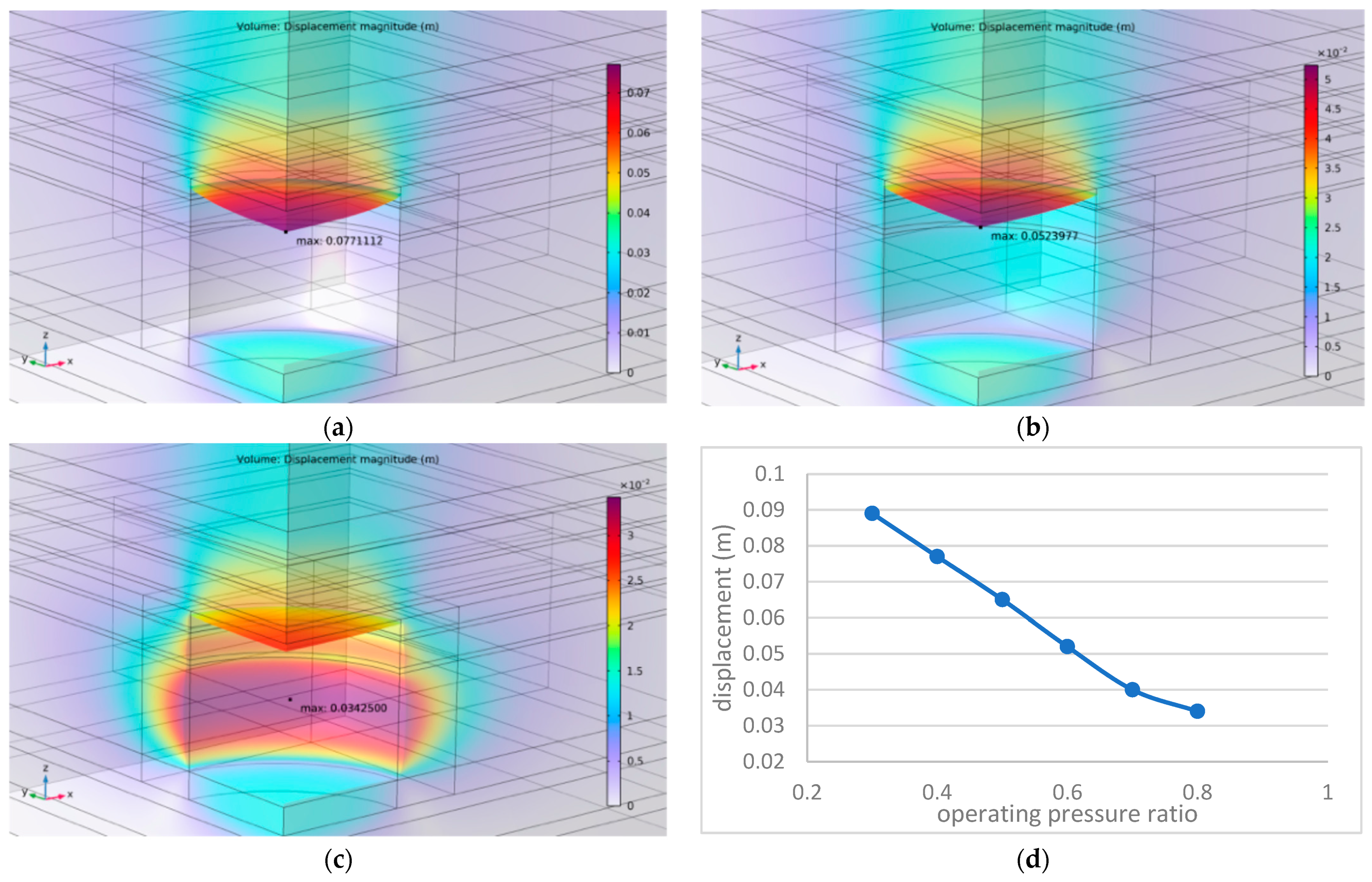
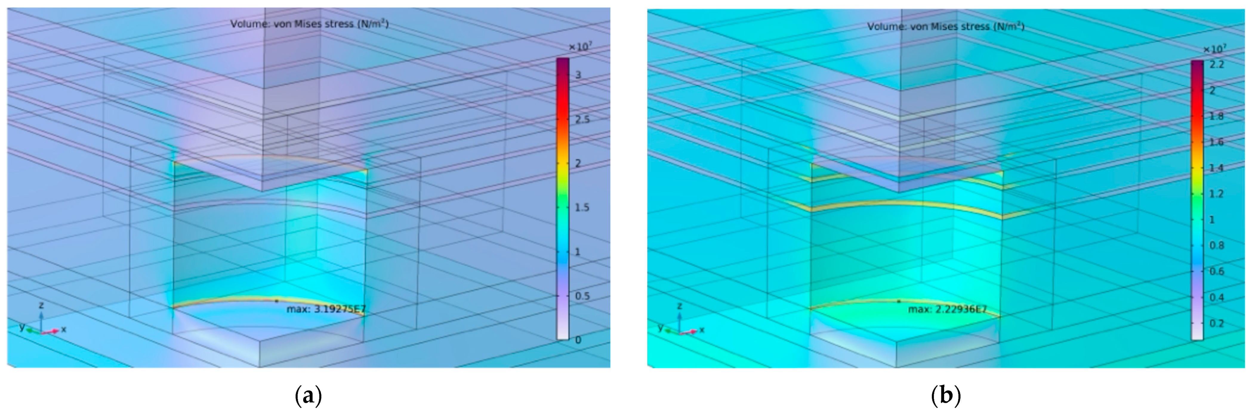
5.2.3. Long-Term Stability Evaluation

The pronounced plastic deformation and creep behavior of salt rock make it essential to evaluate the long-term stability of salt caverns, as the cyclic loading and unloading process will inevitably introduce unwanted deformation and even damage. To further support the operating pressure range, long-term stability evaluations considering both the creep effect and the plastic deformation of the salt rock are conducted. The simulation considers 10 years of operation, and maximum operating pressures of 0.6, 0.7, and 0.8 times the vertical stress are chosen. The relevant rock properties are shown in

Table 4. Creep properties for rock layers.

Lithology	Creep Rate Coefficient (1/s)	Stress Exponent	Reference Stress (MPa)
Shale	5 × 10−15	3.24	1.0
Salt	1.415 × 10−14	3.52	1.0
Anhydrite	3.3 × 10−15	3.16	1.0
Limestone	4.8 × 10−15	4	1.0

.

Figure 15 illustrates the plastic deformation contour after the simulation. It is noteworthy that since the deformation of the sediment will not harm the overall stability of the cavern, the sediment layer is not shown in the picture for a clearer view.

According to Figure 15, after 10 years of the loading cycle, the plastic deformation demonstrates an uneven distribution. For cases with a maximum operating pressure ratio of 0.6 and 0.7, plastic deformation is primarily concentrated along the sidewall near the top of the sediment layer, as the connecting corner induces stress concentration. Around the cavern bottom, plastic strain is primarily concentrated along the x-axis, the y-axis, and the central region between these directions. As the operating pressure is uniformly applied to the cavern wall, the directions aligned with the horizontal principal stress retain higher stress levels, leading to greater deformation in these areas. For caverns with a maximum operating pressure ratio of 0.7, the most prominent plastic deformation occurs in the middle region between the x-axis and y-axis directions, where shear stress is at its highest level. Bearing a weaker shear resistance, the salt rock tends to develop a higher plastic deformation level, thus making it more susceptible to potential structural risks. Though unevenly distributed, the maximum plastic strain stays low, while the surrounding areas exhibit minimal plastic deformation. The highly deformed region helps relieve intensified stress, thereby maintaining overall stability within an acceptable range. When the maximum operating pressure ratio reaches 0.8, the shale interlayer loses its stability as extremely high-level plastic deformation occurs, which is around 1000 times higher than that of the surrounding salt rock. Such high deformation will inevitably compromise the overall stability of the cavern, potentially leading to failure in the interlayers.

Figure 16 shows the creep strain distribution after simulation.

As shown in Figure 16, the cavern wall near the sediment layer top develops a concentrated creep strain region, corresponding to the stress concentration region when the cavern is subjected to operating pressure. The maximum creep strain for the cavern with a maximum operating pressure ratio of 0.6 is significantly high, making the cavern corner in the direction of the maximum horizontal stress a potential zone of failure. This further corroborates the stationary simulation result that the applied operating pressure helps relieve the stress concentration, making the maximum von Mises stress higher, with minor average operating pressure. For the case with a maximum operating pressure ratio of 0.7, the maximum creep strain is found where the maximum shear stress occurs, as the shear stress concentration makes the salt rock reach its shear residence limit. However, the creep strain in most of the cavern stays minimal, averaging 0.2%, and the average creep strain in the corner stays around 2%, which is an acceptable value. Moreover, when leaching the salt cavern, the sediment layer will be less condensed; thus, a curve will most likely form in the corner, relieving the stress concentration. Therefore, the cavern is still considered stable in this case. When the maximum operating ratio reaches 0.8, the average creep strain in the corner increases, and the shale layer and salt rock around develop significant creep deformation due to the shear stress concentration and compression. The maximum creep strain in the shale layer reaches 14.4%, indicating significant deformation and a potential risk of failure.

Overall, the range for the operating pressure of between 0.4 and 0.7 times the vertical stress strikes a balance between minimizing leakage and maintaining the structural stability of the cavern.

6. Conclusions

Based on the stratigraphy characteristics of the B unit of the Salina group in Southern Ontario, Canada, simulations have been performed to optimize essential parameters for CAES in salt cavern design, focusing on different cavern shapes and operating pressures. Two main shapes, cylinder and ellipsoid, are analyzed in this study, and the impacts of diameter are considered for cavern shape optimization. The comparison study results indicate that the cylinder-shaped cavern with a diameter 1.5 times its height shows large storage potential while maintaining good stability. While the ellipsoidal shape effectively reduces stress concentration, it also leads to increased deformation in the shale interlayers, and the insoluble content makes the shape around the shale layers hard to control.

Stationary simulations of varying operating pressures reveal that an appropriate operating pressure helps mitigate stress concentration at the cavern corners by enlarging the corner angle. However, excessive operating pressure results in significant deformation and may cause tensile failure at the cavern walls. The minimum operating pressure ratio is optimized at 0.4, as lower pressures fail to effectively reduce stress concentration. A maximum operating pressure ratio of 0.7 is recommended, while 0.6 and 0.8 may be set as the reference group for further analysis. Based on the results, tightness evaluation and plastic-creep simulations are conducted to further optimize the operating pressure. The tightness evaluation indicates that all three cases exhibit minimal leakage rates, with the rate of capacity increase surpassing the rate of leakage mass increase. The plastic-creep simulation results demonstrate that shear stress concentration accelerates the sidewall deformation at a maximum operating pressure ratio of 0.7, but the cavern maintains good overall stability, as most of the cavern deformation remains minor. When the maximum operating pressure ratio grows to 0.8, significant deformation occurs at the shale layers. These results further corroborate the conclusion that the optimal operating pressure range is 0.4–0.7 times the vertical stress.

7. Discussion

While this study provides a preliminary assessment of implementing CAES systems in salt deposits in southern Ontario, further research is required before construction can proceed. To begin with, while this study conducts a 10-year time span of the cavern’s creep and plastic deformation, fatigue behavior is not considered. Salty rocks exhibit both creep deformation and fatigue during the cyclic loading process; thus, only considering the creep factor may lead to an incomplete understanding of the cavern’s behavior during prolonged operations. Future studies should incorporate both creep and fatigue simulations to provide a more comprehensive assessment. Moreover, due to limited access to detailed geological data, this study relies on data representative of typical rock formations found in both Canada and China. Field experiments may also be incorporated to provide more precise geographical and geological data for validation. Practical aspects like economic impact will also be studied in future research. Furthermore, future studies will focus on more sophisticated energy storage and withdrawal strategies, resulting in a more realistic and detailed framework.

References

1. Hansen, J.E.; Sato, M.; Simons, L.; Nazarenko, L.S.; Sangha, I.; Kharecha, P.; Zachos, J.C.; von Schuckmann, K.; Loeb, N.G.; Osman, M.B.; et al. Global Warming in the Pipeline. Oxf. Open Clim. Change 2023, 3, kgad008. [Google Scholar] [CrossRef]
2. NICR 2013-05 US Nat Resources 2020, 2030 2040.Pdf. Available online: https://www.dni.gov/files/documents/NICR%202013-05%20US%20Nat%20Resources%202020%2C%202030%202040.pdf?utm_source=chatgpt.com (accessed on 18 February 2025).
3. Global Overview—Renewables 2024—Analysis. IEA. Available online: https://www.iea.org/reports/renewables-2024/global-overview (accessed on 18 February 2025).
4. Japan Adopts New Carbon Reduction Targets as It Plans to Boost Nuclear and Renewable Energy by 2040|AP News. Available online: https://apnews.com/article/japan-climate-energy-decarbonization-targets-nuclear-carbon-7006f2dd241e30a3129a00da5bf707dd (accessed on 18 February 2025).
5. Europe Posts Record Year for Clean Energy Use as Trump Pulls US Toward Fossil Fuels. AP News. Available online: https://apnews.com/article/europe-renewables-climate-change-solar-wind-fossil-fuels-4a6ff96bbde3251cb42109e1d9d4b399 (accessed on 18 February 2025).
6. Fariza, I. Cold Without Wind: German ‘Dunkelflaute’ Brings Electricity Prices to Crisis Levels and Depletes Gas Reserves. EL PAÍS English. Available online: https://english.elpais.com/international/2024-12-12/cold-without-wind-german-dunkelflaute-brings-electricity-prices-to-crisis-levels-and-depletes-gas-reserves.html (accessed on 19 February 2025).
7. Malka, L.; Daci, A.; Kuriqi, A.; Bartocci, P.; Rrapaj, E. Energy Storage Benefits Assessment Using Multiple-Choice Criteria: The Case of Drini River Cascade, Albania. Energies 2022, 15, 4032. [Google Scholar] [CrossRef]
8. Zou, P.; Chen, Q.; Yu, Y.; Xia, Q.; Kang, C. Electricity Markets Evolution with the Changing Generation Mix: An Empirical Analysis Based on China 2050 High Renewable Energy Penetration Roadmap. Appl. Energy 2017, 185, 56–67. [Google Scholar] [CrossRef]
9. Evans, A.; Strezov, V.; Evans, T.J. Assessment of Utility Energy Storage Options for Increased Renewable Energy Penetration. Renew. Sustain. Energy Rev. 2012, 16, 4141–4147. [Google Scholar] [CrossRef]
10. Li, H.; Ma, H.; Zhao, K.; Zhu, S.; Yang, K.; Zeng, Z.; Zheng, Z.; Yang, C. Parameter Design of the Compressed Air Energy Storage Salt Cavern in Highly Impure Rock Salt Formations. Energy 2024, 286, 129520. [Google Scholar] [CrossRef]
11. Nikolaos, P.C.; Marios, F.; Dimitris, K. A Review of Pumped Hydro Storage Systems. Energies 2023, 16, 4516. [Google Scholar] [CrossRef]
12. Shah, M.; Prajapati, M.; Yadav, K.; Sircar, A. A Comprehensive Review of Geothermal Energy Storage: Methods and Applications. J. Energy Storage 2024, 98, 113019. [Google Scholar] [CrossRef]
13. Takach, M.; Sarajlić, M.; Peters, D.; Kroener, M.; Schuldt, F.; von Maydell, K. Review of Hydrogen Production Techniques from Water Using Renewable Energy Sources and Its Storage in Salt Caverns. Energies 2022, 15, 1415. [Google Scholar] [CrossRef]
14. Rabi, A.M.; Radulovic, J.; Buick, J.M. Comprehensive Review of Compressed Air Energy Storage (CAES) Technologies. Thermo 2023, 3, 104–126. [Google Scholar] [CrossRef]
15. Li, L.; Liang, W.; Lian, H.; Yang, J.; Dusseault, M. Compressed Air Energy Storage: Characteristics, Basic Principles, and Geological Considerations. Adv. Geo-Energy Res. 2018, 2, 135–147. [Google Scholar] [CrossRef]
16. Tarkowski, R. Underground Hydrogen Storage: Characteristics and Prospects. Renew. Sustain. Energy Rev. 2019, 105, 86–94. [Google Scholar] [CrossRef]
17. Wan, J.; Sun, Y.; He, Y.; Ji, W.; Li, J.; Jiang, L.; Jurado, M.J. Development and Technology Status of Energy Storage in Depleted Gas Reservoirs. Int. J. Coal. Sci. Technol. 2024, 11, 29. [Google Scholar] [CrossRef]
18. Zheng, Z.; Wang, G.; Yang, C.; Ma, H.; Yin, L.; Liao, Y.; Zhao, K.; Zeng, Z.; Li, H.; Han, Y. A Novel Nano-Grade Organosilicon Polymer: Improving Airtightness of Compressed Air Energy Storage in Hard Rock Formations. Int. J. Min. Sci. Technol. 2024, 34, 305–321. [Google Scholar] [CrossRef]
19. Guo, C.; Zhang, K.; Pan, L.; Cai, Z.; Li, C.; Li, Y. Numerical Investigation of a Joint Approach to Thermal Energy Storage and Compressed Air Energy Storage in Aquifers. Appl. Energy 2017, 203, 948–958. [Google Scholar] [CrossRef]
20. Donadei, S.; Schneider, G.-S. Compressed Air Energy Storage in Underground Formations. In Storing Energy; Elsevier: Amsterdam, The Netherlands, 2016. [Google Scholar] [CrossRef]
21. King, M.; Jain, A.; Bhakar, R.; Mathur, J.; Wang, J. Overview of Current Compressed Air Energy Storage Projects and Analysis of the Potential Underground Storage Capacity in India and the UK. Renew. Sustain. Energy Rev. 2021, 139, 110705. [Google Scholar] [CrossRef]
22. Fertig, E.; Apt, J. Economics of Compressed Air Energy Storage to Integrate Wind Power: A Case Study in ERCOT. Energy Policy 2011, 39, 2330–2342. [Google Scholar] [CrossRef]
23. Yin, J.; Zhan, X. Impact of Bias-Correction Methods on Effectiveness of Assimilating SMAP Soil Moisture Data into NCEP Global Forecast System Using the Ensemble Kalman Filter. IEEE Geosci. Remote Sens. Lett. 2018, 15, 659–663. [Google Scholar] [CrossRef]
24. Mou, J.; Shang, H.; Ji, W.; Wan, J.; Xing, T.; Ma, H.; Peng, W. Feasibility Analysis of Compressed Air Energy Storage in Salt Caverns in the Yunying Area. Energies 2023, 16, 7171. [Google Scholar] [CrossRef]
25. Zhao, H.; Hao, X. Risk Assessment of Zero-Carbon Salt Cavern Compressed Air Energy Storage Power Station. J. Clean. Prod. 2024, 468, 143002. [Google Scholar] [CrossRef]
26. Dooner, M.; Wang, J. Potential Exergy Storage Capacity of Salt Caverns in the Cheshire Basin Using Adiabatic Compressed Air Energy Storage. Entropy 2019, 21, 1065. [Google Scholar] [CrossRef]
27. Lemieux, A.; Shkarupin, A.; Sharp, K. Geologic Feasibility of Underground Hydrogen Storage in Canada. Int. J. Hydrogen Energy 2020, 45, 32243–32259. [Google Scholar] [CrossRef]
28. Li, L.; Yin, S.; Wang, Z. A Preliminary Assessment of Underground Space Resources for Hydrogen Storage in Salt Caverns in Lambton County, Southern Ontario, Canada. Mining 2024, 4, 530–545. [Google Scholar] [CrossRef]
29. Rine, M.J.; McLaughlin, P.I.; Bancroft, A.M.; Harrison, W.B.; Kuglitsch, J.; Caruthers, A.H.; Ramezani, J.; Kaczmarek, S.E.; Emsbo, P. Linked Silurian Carbon Cycle Perturbations, Bursts of Pinnacle Reef Growth, Extreme Sea-Level Oscillations, and Evaporite Deposition (Michigan Basin, USA). Palaeogeogr. Palaeoclimatol. Palaeoecol. 2020, 554, 109806. [Google Scholar] [CrossRef]
30. Carter, T. Bedded Salt in Ontario: Geology, Solution Mining and Cavern Storage. Available online: https://www.ogsrlibrary.com/downloads/Salt-Geology-and-Cavern-Storage-OPI-2009.pdf (accessed on 4 November 2024).
31. Drucker-Prager Criterion—ProQuest. Available online: https://www.proquest.com/docview/1114283355?accountid=14906&parentSessionId=0O9lmQYtpEmaQrytQSxrvu%2BeWyUhsFF82rIAZqnZ%2FQw%3D&pq-origsite=primo&sourcetype=Scholarly%20Journals (accessed on 4 November 2024).
32. Liu, W.; Dong, Y.; Zhang, Z.; Li, L.; Jiang, D.; Fan, J.; Chen, J.; Zhang, X.; Wan, J.; Li, Z. Optimization of Operating Pressure of Hydrogen Storage Salt Cavern in Bedded Salt Rock with Multi-Interlayers. Int. J. Hydrogen Energy 2024, 58, 974–986. [Google Scholar] [CrossRef]
33. Chromik, M.; Korzeniowski, W. A Method to Increase the Leaching Progress of Salt Caverns with the Use of the Hydro-Jet Technique. Energies 2021, 14, 5833. [Google Scholar] [CrossRef]
34. Cyran, K. Insight Into a Shape of Salt Storage Caverns. Arch. Min. Sci. 2020, 65, 363–398. [Google Scholar] [CrossRef]
35. Małachowska, A.; Łukasik, N.; Mioduska, J.; Gębicki, J. Hydrogen Storage in Geological Formations—The Potential of Salt Caverns. Energies 2022, 15, 5038. [Google Scholar] [CrossRef]
36. Caglayan, D.G.; Weber, N.; Heinrichs, H.U.; Linßen, J.; Robinius, M.; Kukla, P.A.; Stolten, D. Technical Potential of Salt Caverns for Hydrogen Storage in Europe. Int. J. Hydrogen Energy 2020, 45, 6793–6805. [Google Scholar] [CrossRef]
37. Parkes, D.; Evans, D.J.; Williamson, P.; Williams, J.D.O. Estimating Available Salt Volume for Potential CAES Development: A Case Study Using the Northwich Halite of the Cheshire Basin. J. Energy Storage 2018, 18, 50–61. [Google Scholar] [CrossRef]
38. Williams, J.D.O.; Williamson, J.P.; Parkes, D.; Evans, D.J.; Kirk, K.L.; Sunny, N.; Hough, E.; Vosper, H.; Akhurst, M.C. Does the United Kingdom Have Sufficient Geological Storage Capacity to Support a Hydrogen Economy? Estimating the Salt Cavern Storage Potential of Bedded Halite Formations. J. Energy Storage 2022, 53, 105109. [Google Scholar] [CrossRef]
39. Ma, L.; Wang, M.; Zhang, N.; Fan, P.; Li, J. A Variable-Parameter Creep Damage Model Incorporating the Effects of Loading Frequency for Rock Salt and Its Application in a Bedded Storage Cavern. Rock Mech. Rock Eng. 2017, 50, 2495–2509. [Google Scholar] [CrossRef]
40. Zhou, Y.; Xia, C.; Zhao, H.; Mei, S.; Zhou, S. An Iterative Method for Evaluating Air Leakage from Unlined Compressed Air Energy Storage (CAES) Caverns. Renew. Energy 2018, 120, 434–445. [Google Scholar] [CrossRef]
41. Zhao, K.; Liu, Y.; Li, Y.; Ma, H.; Hou, W.; Yu, C.; Liu, H.; Feng, C.; Yang, C. Feasibility Analysis of Salt Cavern Gas Storage in Extremely Deep Formation: A Case Study in China. J. Energy Storage 2022, 47, 103649. [Google Scholar] [CrossRef]
42. Ozarslan, A. Large-Scale Hydrogen Energy Storage in Salt Caverns. Int. J. Hydrogen Energy 2012, 37, 14265–14277. [Google Scholar] [CrossRef]
Figure 1. Detailed lithology distribution of the Salina Formation. The same color indicates the same rock type, while the red box highlights the stratum corresponding to Unit B [28].
Energies 18 02258 g001
Figure 2. The core distributions and subunits of unit B. Data taken from the F006864 well (left) and T003039 well (right). The green dotted line represents the mean value of the neutron log [28].
Energies 18 02258 g002
Figure 3. The north–south variation in thickness of subunits SQ1, SQ2, and SQ3 [28].
Energies 18 02258 g003
Figure 4. Salt cavern schematic showing different dissolution setups. (Left): direct leaching; (right): indirect leaching.
Energies 18 02258 g004
Figure 5. Stress field after cylinder-shaped caverns with different diameter–height ratios are excavated, (a) ratio = 0.5, (b) ratio = 1, (c) ratio = 1.5, (d) ratio = 2.0, (e) ratio = 2.5, (f) maximum von Mises stress curve corresponding to different ratios.
Energies 18 02258 g005
Figure 6. Displacement contour after cylinder-shaped caverns with different diameter–height ratios are excavated, (a) ratio = 0.5, (b) ratio = 1, (c) ratio = 1.5, (d) ratio = 2.0, (e) ratio = 2.5, (f) maximum displacement curve corresponding to different ratios.
Energies 18 02258 g006
Figure 7. Plastic strain contour after cylinder-shaped caverns with different diameter–height ratios are excavated, (a) ratio = 0.5, (b) ratio = 1, (c) ratio = 1.5, (d) ratio = 2.0, (e) ratio = 2.5, (f) maximum plastic strain curve corresponding to different ratios.
Energies 18 02258 g007
Figure 8. Stress field after ellipsoid-shaped caverns with different diameter–height ratios are excavated, (a) ratio = 0.5, (b) ratio = 1, (c) ratio = 1.5, (d) ratio = 2.0, (e) ratio = 2.5, (f) maximum von Mises stress curve corresponding to different ratios.
Energies 18 02258 g008aEnergies 18 02258 g008b
Figure 9. Displacement contour after ellipsoid-shaped caverns with different diameter–height ratios are excavated, (a) ratio = 0.5, (b) ratio = 1, (c) ratio = 1.5, (d) ratio = 2.0, (e) ratio = 2.5, (f) maximum displacement curve corresponding to different ratios.
Energies 18 02258 g009
Figure 10. Plastic strain contour after ellipsoid-shaped caverns with different diameter–height ratios are excavated, (a) ratio = 0.5, (b) ratio = 1, (c) ratio = 1.5, (d) ratio = 2.0, (e) ratio = 2.5, (f) maximum plastic strain curve corresponding to different ratios.
Energies 18 02258 g010
Figure 11. Displacement contours at different operating pressure-to-vertical stress ratios, (a) ratio = 0.4, (b) ratio = 0.6, (c) ratio = 0.8, (d) maximum von Mises stress curve corresponding to different ratios.
Energies 18 02258 g011
Figure 12. Von Mises stress distribution at different operating pressure-to-vertical stress ratios, (a) ratio = 0.4, (b) ratio = 0.6, (c) ratio = 0.8, (d) maximum von Mises stress curve corresponding to different ratios.
Energies 18 02258 g012aEnergies 18 02258 g012b
Figure 13. Pore pressure distribution at the end of the simulation, (a) ratio = 0.7, (b) maximum pore pressure curve corresponding to different ratios.
Energies 18 02258 g013
Figure 14. Leakage rate after 10 years.
Energies 18 02258 g014
Figure 15. Plastic strain distribution at different maximum operating pressure-to-vertical stress ratios, (a) ratio = 0.6, (b) ratio = 0.7, (c) ratio = 0.8.
Energies 18 02258 g015
Figure 16. Equivalent creep strain distribution at different maximum operating pressure-to-vertical stress ratios, (a) ratio = 0.6, (b) ratio = 0.7, (c) ratio = 0.8.
Energies 18 02258 g016