An Improved Short-Term Electricity Load Forecasting Method: The VMD–KPCA–xLSTM–Informer Model

Abstract

This paper proposes a hybrid forecasting method (VMD–KPCA–xLSTM–Informer) based on variational-mode decomposition (VMD), kernel principal component analysis (KPCA), extended long short-term memory network (xLSTM), and the Informer model. First, the method decomposes the original power load data and environmental parameter data using VMD to capture their multi-scale characteristics. Next, KPCA extracts nonlinear features and reduces the dimensionality of the decomposed modals to eliminate redundant information while retaining key features. The xLSTM network then models temporal dependencies to enhance the model’s memory capability and prediction accuracy. Finally, the Informer model processes long-sequence data to improve prediction efficiency. Experimental results demonstrate that the VMD–KPCA–xLSTM–Informer model achieves an average absolute percentage error (MAPE) as low as 2.432% and a coefficient of determination ($R^2$) of 0.9532 on dataset I, while, on dataset II, it attains a MAPE of 4.940% and an $R^2$ of 0.8897. These results confirm that the method significantly improves the accuracy and stability of short-term power load forecasting, providing robust support for power system optimization.

1. Introduction

Power load forecasting is a key link in power system planning, operation, and economic management and plays an important role in securing power supply, improving system efficiency, and reducing costs. Due to numerous external influences, power load presents complex nonlinear and time-varying characteristics, making short-term power load forecasting a difficult task. This complexity makes the development and use of forecasting models even more challenging [1].

There are various methods for power load forecasting, which can be mainly categorized into time-series analysis methods, machine learning methods, and deep learning methods. The time-series analysis method is one of the earliest methods used for power load forecasting; it is mainly based on using historical data to construct mathematical models to describe the relationship between time and load values. Common models include autoregressive integrated moving-average model (ARIMA) [2], seasonal autoregressive integrated moving-average model (SARIMA) [3], and vector autoregression model (VAR) [4]. When applied to power load forecasting, the time-series analysis method has the advantages of easy operation, high computational efficiency, and the ability to effectively capture the seasonal and trend characteristics of the data. However, the method has obvious limitations, such as harsh assumptions, difficulty in dealing with complex nonlinear relationships, extreme sensitivity to outliers, relatively narrow prediction range, and its insufficient consideration of external influences. In the case of strong data volatility, the time-series analysis method fails to accurately predict future data due to strong assumptions, and the MAPE reaches 14.5 [5,6]. Machine learning methods are able to deal with complex nonlinear relationships by automatically extracting features from a large amount of data, and common models include support vector machine (SVM) [7], Random Forests [8], extreme gradient boosting (XGBoost) [9], and least absolute shrinkage and selection operator (Lasso) [10]. Compared with time-series analysis methods, machine learning methods can improve the prediction accuracy, but there are still deficiencies in the extraction of data features, and, when faced with complex power systems, their prediction effect is poor and the accuracy of power load prediction is low [11,12]. The machine learning method has an R² of 0.75 and a MAPE of 5.70% when dealing with complex power system data, which are much lower than expected [13]. Deep learning models, on the other hand, are able to capture complex patterns through multilevel nonlinear transformations, and common models include artificial neural network (ANN) [14], long short-term memory (LSTM) [15], convolutional neural network (CNN) [16], and bidirectional long short-term memory (Bi-LSTM) [17]. Long short-term memory networks are specifically designed to deal with long-term dependency problems and are particularly suitable for the prediction of time-series data. And a bidirectional long short-term memory network combined with K-Means clustering and the Transformer model can further improve the prediction accuracy.

In the 1990s, the cyclic error-correcting code gating mechanism was introduced as the core idea of long short-term memory (LSTM) networks. Since then, LSTM has stood the test of time and contributed to many successful deep learning applications. However, the emergence of Transformer technology, which is centered on a parallelizable self-attention mechanism, marks the beginning of a new era and has surpassed LSTM in large-scale applications. Based on the LSTM model, literature reference [18] extends LSTM to billions of parameters and utilizes the latest technology of modern LLM, while alleviating the known limitations of LSTM, proposing the extended long short-term memory model. The xLSTM significantly enhances its modeling ability for long sequences by introducing exponential gating and an improved memory structure. This makes the xLSTM excel in both performance and scalability when compared to state-of-the-art Transformers and state-space models for processing complex time-series predictions.

Traditional Transformer models face problems of computational complexity and memory consumption when processing long sequences of data. Therefore, the research team from Peking University proposed Informer, a time-series prediction model based on the Transformer architecture [19]. By introducing the ProbSparse self-attention mechanism and distillation mechanism, the computational and memory efficiency of the model is significantly improved. It excels at processing long sequences of data, can capture long-distance dependencies, and has achieved excellent performance in multiple time-series prediction tasks.

Power load data may contain multiple frequency components and noise. The direct modeling of complex signals can lead to difficult model training and poor prediction accuracy. Many scholars process the data before prediction to improve prediction accuracy. Paper [20] proposes an EMD–ISSA–LSTM short-term power load prediction model based on empirical mode decomposition (EMD) and an improved sparrow search algorithm (ISSA). However, EMD is prone to mode aliasing during decomposition and is sensitive to noise. Compared with EMD, variational mode decomposition can suppress mode aliasing and is noise-resistant by means of a frequency-domain bandwidth constraint mechanism and minimizing the bandwidth of the mode components.

Ref. [21] uses the VMD–Pyraformer–Adan model for prediction. First, the VMD algorithm is used to decompose the load data into modal components of different frequencies. The zero-crossing rate and Pearson correlation coefficient are introduced to divide the modal components, obtaining low-frequency, medium-frequency, and high-frequency components, which are combined with the original load data to form reconstructed data. Next, the reconstructed data are input into the Pyraformer prediction network, and the parameters are optimized using the Adan optimizer to finally output the prediction results. Experimental results show that, compared with existing models, this model has higher prediction accuracy, but the input data are only the load data after decomposition by VMD, and environmental parameter data, such as temperature, humidity, wind speed, rainfall, etc., which are important variables affecting power demand, are not considered. If these environmental factors are not considered, the prediction results will be inaccurate. In [22], the VMD–KPCA–WSO–LSTM model was used to predict photovoltaic power. First, the VMD method was used to decompose the environmental factor sequence to reduce the non-stationarity of the sequence. Then, the kernel principal component analysis method was used to extract the characteristic sequence of the main influencing factors to obtain the best meteorological characteristic sequence. Finally, an LSTM network is used to predict the multivariate feature sequence, and a white shark optimization algorithm is used to optimize the parameters of the long short-term memory network to achieve the accurate prediction of photovoltaic output. However, considering only environmental factors and not historical data will cause the model to be unable to use historical trend information and the statistical characteristics of historical data, which will reduce the accuracy and reliability of the prediction results.

Current power load forecasting technology uses deep learning as its core, employing models like LSTM, BiLSTM, and Transformer to capture time-series features. These approaches are often combined with signal decomposition methods such as CEEMDAN and VMD to reduce data non-stationarity, thereby improving prediction accuracy significantly. To address the challenges of strong load variability and fluctuations under extreme weather, research prioritizes multi-frequency band feature extraction [23] and dynamic feature screening. Additionally, hybrid physical–data-driven models are introduced to enhance scenario adaptability. Despite advancements in feature engineering and model fusion, existing methods still struggle with bottlenecks like low computational efficiency and insufficient generalization for small-sample cases [24]. Future trends will focus on breakthroughs in large language model-based small-sample transfer learning, the multivariate joint prediction of electricity source–load–price, and probabilistic uncertainty quantification. These innovations will integrate with edge computing’s lightweight deployment, driving prediction technology toward high robustness, real-time performance, and multimodal fusion. Ultimately, such evolution aims to support the safe, stable operation of new power systems.

Based on the above analysis, this paper proposes a short-term power load forecasting model based on VMD–KPCA–xLSTM–Informer. The VMD–KPCA framework synergistically optimizes signal decomposition and nonlinear feature dimensionality reduction to enhance input data robustness. The improved xLSTM component strengthens dynamic adaptability to abrupt loads through gating optimization. Simultaneously, the Informer module efficiently captures long-period load patterns via its ProbSparse self-attention mechanism. By integrating decomposition with dimensionality reduction, time-series optimization, and long-sequence modeling, the model achieves complementary advantages. It significantly improves prediction accuracy and computational efficiency in high-fluctuation scenarios. Furthermore, it addresses the limitations of traditional methods in complex nonlinear coupling environments. This work provides a more universal solution for power systems to manage multi-source uncertainty.

2. Basic Model Principle

2.1. Variational Mode Decomposition

VMD is an adaptive signal decomposition method used to decompose a complex signal into multiple mode components (IMFs), each with a specific center frequency and bandwidth. It overcomes the problems of mode aliasing and endpoint effects of traditional methods such as EMD. It can more accurately extract the intrinsic modes of a signal through variational framework optimization and is suitable for processing nonlinear and non-stationary signals. VMD constructs a constrained variational problem to decompose a signal into K modal components, each of which is compactly distributed around the center frequency. The mathematical model is shown in Equation (1):

$$\underset{\left\{u_k\right\},\left\{{\omega }_k\right\}}{min}\left\{\sum _{k=1}^K{∥{\partial }_t\left[\left(\delta \left(t\right)+{\displaystyle \frac{j}{\pi t}}\right)\ast u_k\left(t\right)\right]e^{-j{\omega }_{k}t}∥}_2^2\right\}$$

(1)

The constraints are as follows:

$$\sum _{k=1}^K{u}_k\left(t\right)=f\left(t\right)$$

(2)

where $u_k\left(t\right)$ is the kth modal component, ${\omega }_k$ is the center frequency, $\delta \left(t\right)$ is the unit impulse function, ${\partial }_t$ is the time derivative of the function, “∗” denotes the convolution operation, $e^{-j{\omega }_{k}t}$ is the modulation term, and $f\left(t\right)$ is the original signal.

VMD transforms the problem into an unconstrained optimization problem by constructing a constrained variational optimization problem and introducing Lagrange multipliers and penalty factors. Each modal component $u_k$ is first updated by the alternating direction multiplier method:

$$u_k^{n+1}\left(\omega \right)={\displaystyle \frac{f\left(\omega \right)-{\sum }_{i\ne k}{u}_i\left(\omega \right)+\frac{\lambda \left(\omega \right)}{2}}{1+2\alpha {\left(\omega -{\omega }_k\right)}^2}}$$

(3)

where $f\left(\omega \right)$ is the frequency-domain representation of the original signal, $u_k\left(\omega \right)$ is the frequency-domain representation of the kth mode, $\lambda \left(\omega \right)$ is the frequency-domain representation of the Lagrange multiplier, and $\alpha$ is the bandwidth control parameter. The center frequency ${\omega }_k$ is then updated according to the spectral properties of the modal components:

$${\omega }_k^{n+1}={\displaystyle \frac{{\int }_0^{\infty }\omega {\left|u_k\left(\omega \right)\right|}^{2}d\omega }{{\int }_0^{\infty }{\left|u_k\left(\omega \right)\right|}^{2}d\omega }}$$

(4)

Then, update the Lagrange multipliers $\lambda$ to enhance the constraints:

$${\lambda }^{n+1}\left(\omega \right)={\lambda }^n\left(\omega \right)+\tau \left(f\left(\omega \right)-\sum _k{u}_k^{n+1}\left(\omega \right)\right)$$

(5)

where $\tau$ is the update step. Finally, check whether the algorithm satisfies the convergence conditions. The convergence conditions include whether the update of the modal component $u_k$ is stabilized:

$$\sum _k{∥u_k^{n+1}-u_k^n∥}_2^2<{ϵ}_1$$

(6)

whether the update of the center frequency ${\omega }_k$ is stabilizing:

$$\sum _k{∥{\omega }_k^{n+1}-{\omega }_k^n∥}_2^2<{ϵ}_2$$

(7)

and whether the update of the Lagrange multiplier $\lambda$ stabilizes:

$${∥{\lambda }^{n+1}-{\lambda }^n∥}_2^2<{ϵ}_3$$

(8)

where ${ϵ}_1$, ${ϵ}_2$, and ${ϵ}_3$ are three predefined tolerance thresholds. If all the above conditions are satisfied, the algorithm converges; otherwise, the iteration continues. The final output is the decomposed modal component $u_k$ and the corresponding center frequency ${\omega }_k$. It has been proven theoretically and experimentally that the algorithm converges quickly and with high stability, which ensures the reliability of the decomposition results [25].

Reconstruction error (RE) is an important indicator of data fidelity when decomposing VMD. It is used to evaluate the difference between the reconstructed signal and the original signal after decomposition. When the reconstruction error is small enough and does not show a significant downward trend, the parameter K can be determined. The specific formula is

$$\mathrm{RE}={\displaystyle \frac{∥f\left(t\right)-{\sum }_{k=1}^K{u}_k\left(t\right)∥}{\parallel f\left(t\right)\parallel }}$$

(9)

where $f\left(t\right)$ is the original signal, $u_k\left(t\right)$ is the kth modal component, K is the total number of modal components, and the denominator $\parallel f\left(t\right)\parallel$ is used for normalization so that the error values are comparable for different signal amplitudes.

2.2. Kernel Principal Component Analysis

KPCA is a nonlinear extension of principal component analysis (PCA) that is used to deal with nonlinear data distributions. Traditional PCA is a linear dimensionality reduction method that cannot effectively capture the nonlinear structure of the data. KPCA maps the data to a high-dimensional feature space through a kernel function, and then performs linear PCA analysis in the high-dimensional space, so that nonlinear features can be extracted and complex data distributions can be dealt with.

First, given a dataset $\left\{{\mathbf{x}}_1,{\mathbf{x}}_2,\dots ,{\mathbf{x}}_n\right\}$, KPCA first calculates the kernel matrix K, where $K_{ij}=k\left({\mathbf{x}}_i,{\mathbf{x}}_j\right)$, and then applies centering to the kernel matrix:

$$\tilde{K}=K-{\mathbf{1}}_{n}K-K{\mathbf{1}}_n+{\mathbf{1}}_{n}K{\mathbf{1}}_n$$

(10)

where ${\mathbf{1}}_n$ is the $n\times n$-matrix with all elements equal to $1/n$. The centralizer kernel matrix is then decomposed into eigenvalues:

$$\tilde{K}\mathbf{v}=\lambda \mathbf{v}$$

(11)

where $\lambda$ is the eigenvalue and $\mathbf{v}$ is the corresponding eigenvector. The eigenvectors corresponding to the top k eigenvalues are selected as the principal components. Finally, the data are projected onto the principal component space to obtain the reduced-dimensional data ${\mathbf{y}}_i$:

$${\mathbf{y}}_i=\sum _{j=1}^n{v}_{ij}k\left({\mathbf{x}}_j,{\mathbf{x}}_i\right)$$

(12)

where $v_{ij}$ is the jth component of the ith feature vector and $k\left({\mathbf{x}}_j,{\mathbf{x}}_i\right)$ represents the nuclear function. The reduced-dimensional data retain the main nonlinear characteristics of the original data while greatly reducing the dimension.

Power load data usually have nonlinear and nonsmooth characteristics, and the choice of RBF kernel function can map the data to a high-dimensional space, thus capturing the nonlinear relationships in the data, which are suitable for processing complex power load data. Compared with other kernel functions, the RBF kernel function performs well in tasks such as classification, regression, clustering, and dimensionality reduction.

2.3. Extended Long Short-Term Memory Network

LSTM is a classical recurrent neural network (RNN), which solves the gradient vanishing problem of traditional RNNs by introducing gating mechanisms (input gate, forgetting gate, and output gate), and is able to effectively handle long-sequence data (Figure 1). However, LSTM still has the limitations of (1) limited ability to memorize ultra-long sequences; (2) higher computational complexity and slower training speed; (3) insufficient ability to model certain complex nonlinear relationships. Therefore, xLSTM makes the following extensions and improvements on the basis of LSTM:

(1)

Extended Memory Unit

One of the core improvements of xLSTM is the introduction of the Extended Memory Cell, which is updated with the formula

$$c_t=f_t\odot c_{t-1}+i_t\odot {\tilde{c}}_t+e_t\odot m_t$$

(13)

where $c_t$ is the memory cell state at the current time step, “⊙” denotes that the elements correspond to multiplication, $f_t$ is the forgetting gate, $i_t$ is the input gate, ${\tilde{c}}_t$ is the candidate memory cell state, $e_t$ is the gating signal of the extended memory cell, and $m_t$ is the extended memory cell. The limited capacity of memory cells in traditional LSTM makes it difficult to effectively capture periodic patterns in power loads spanning weeks or months, and the extended memory cells can significantly improve long-term memory capacity through chunking design;

(2)

Multi-Layer Gating Mechanism

xLSTM introduces a multi-layer gating mechanism that enhances the representation of the model by stacking multiple gating layers. The gating signal of each layer is calculated by the following equation:

$$g_t^l=\sigma \left(W_g^l\left[h_{t-1},x_t\right]+b_g^l\right)$$

(14)

where l is the number of layers, $\sigma$ is the activation function, $h_{t-1}$ is the historical information from the previous moment, $x_t$ is the current input, and $W_g^l$ and $b_g^l$ are the weights and biases of the lth layer. Electricity load is affected by multiple coupled factors such as temperature, humidity, electricity price, holidays, etc. xLSTM can realize the dynamic selection of input features through the gating mechanism to improve the fitting ability of complex relationships;

(3)

Adaptive Time Step

xLSTM reduces unnecessary computations by dynamically adjusting the time step through an adaptive mechanism. The formula for the adaptive time step is

$$\Delta t=\tau ·\sigma \left(W_{\tau }{h}_{t-1}+b_{\tau }\right)$$

(15)

where $\tau$ is the scaling factor of the time step, and $W_{\tau }$ and $b_{\tau }$ are the weights and biases. Electricity load data contain both high-frequency fluctuations and low-frequency trends, and the adaptive time step allows the model to automatically shorten the step to capture details during critical periods and lengthen the step to reduce computational cost during smooth periods, which improves the forecasting efficiency.

2.4. Informer Network

Informer networks are an improved model based on the Transformer architecture, aiming to solve the problems of high computational complexity and memory usage faced by traditional Transformers when dealing with long sequential data. The core of Informer networks lies in its unique attention mechanism and encoder–decoder structure.

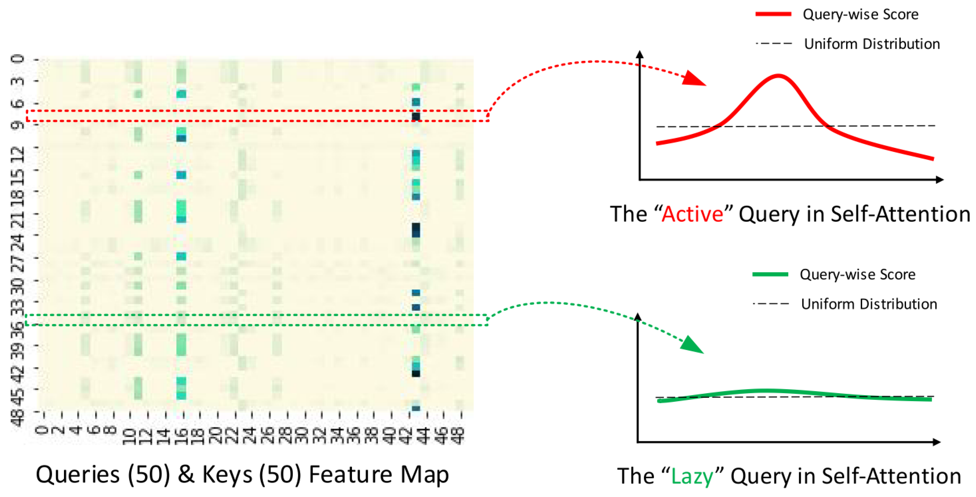
2.4.1. ProbSparse Attention Mechanisms

The ProbSparse attention mechanism is a key feature of the Informer model, which reduces the amount of computation in the self-attention mechanism by probabilizing it to achieve the effective processing of long-sequence time-series data. When the traditional self-attention mechanism calculates the attention score, each query $q_i$ needs to be calculated by dot product with all keys $k_j$. The formula is as follows:

$$A\left(q_i,K,V\right)=\sum _j{\displaystyle \frac{exp\left(q_i{k}_j^{\top }/\sqrt{d}\right)}{{\sum }_{l}exp\left(q_i{k}_l^{\top }/\sqrt{d}\right)}}{v}_j$$

(16)

where $q_i$ is the ith query, K is key matrix, V is value matrix, $k_j$ is the jth key, $v_j$ is the jth value, and d is the input dimension. The computational complexity is $O\left(L^2\right)$ due to the need to compute the dot product over all L queries and L keys, whereas the core idea of the ProbSparse attention mechanism is that not all query–key pairs contribute significantly to the final attention score, and that only a few query–key pairs contribute the majority of the attention score, while the others have a negligible contribution. Thus, the ProbSparse attention mechanism reduces computation by selectively computing those query–key pairs that contribute most to the attention score. To identify which query–key pairs are important, the ProbSparse attention mechanism introduces a sparsity metric $M\left(q_i,K\right)$, which measures the sparsity of the attention distribution of the ith query $q_i$ for all keys K. The sparsity metric $M\left(q_i,K\right)$ is defined as

$$M\left(q_i,K\right)=ln\sum _{j=1}^{L_K}{e}^{q_i{k}_j^{\top }/\sqrt{d}}-{\displaystyle \frac{1}{L_K}}\sum _{j=1}^{L_K}{q}_i{k}_j^{\top }/\sqrt{d}$$

(17)

where the first term is the Log-Sum-Exp (LSE) operation and the second term is the arithmetic average. If $M\left(q_i,K\right)$ is large, tjos means that the attention distribution of this query $q_i$ is sparse and only a few keys contribute significantly to its attention score. To further reduce the computation, the ProbSparse attention mechanism proposes a maximum mean approximation method for the fast estimation of $M\left(q_i,K\right)$. The maximum mean approximation is defined as

$$M\left(q_i,K\right)\approx \underset{j}{max}\left\{q_i{k}_j^{\top }/\sqrt{d}\right\}-{\displaystyle \frac{1}{L_K}}$$

(18)

This approximation avoids computing the dot product of all query–key pairs and instead computes $M\left(q_i,K\right)$ by randomly sampling $U=L_{K}ln{L}_Q$ query–key pairs, thereby reducing the computational complexity from the traditional $O\left(L^2\right)$ to $O(LlnL)$, which reduces the memory footprint when dealing with long sequences of power load data.

The left diagram in Figure 2 shows the feature graph of queries and keys. It can be seen that each query is associated with multiple keys, forming a feature map. The upper right panel in Figure 2 shows the distribution of “active” queries in self-attention. The solid red line represents the query-wise score and the dashed line represents the uniform distribution. It can be seen that the distribution of active query scores shows obvious peaks, indicating that these queries are more active in self-attention and have stronger associations with more keys. By identifying these active queries, the Informer network can more effectively utilize the self-attention mechanism to improve the performance of the model. The lower right panel in Figure 2 shows the distribution of lazy query in self-attention. The green solid line indicates the query score and the dashed line indicates a uniform distribution. It can be seen that the distribution of scores for lazy queries is relatively flat, indicating that these queries are less active in self-attention and less associated with keys. By identifying and processing these lazy queries, the Informer network can reduce unnecessary computations and improve the efficiency of the model.

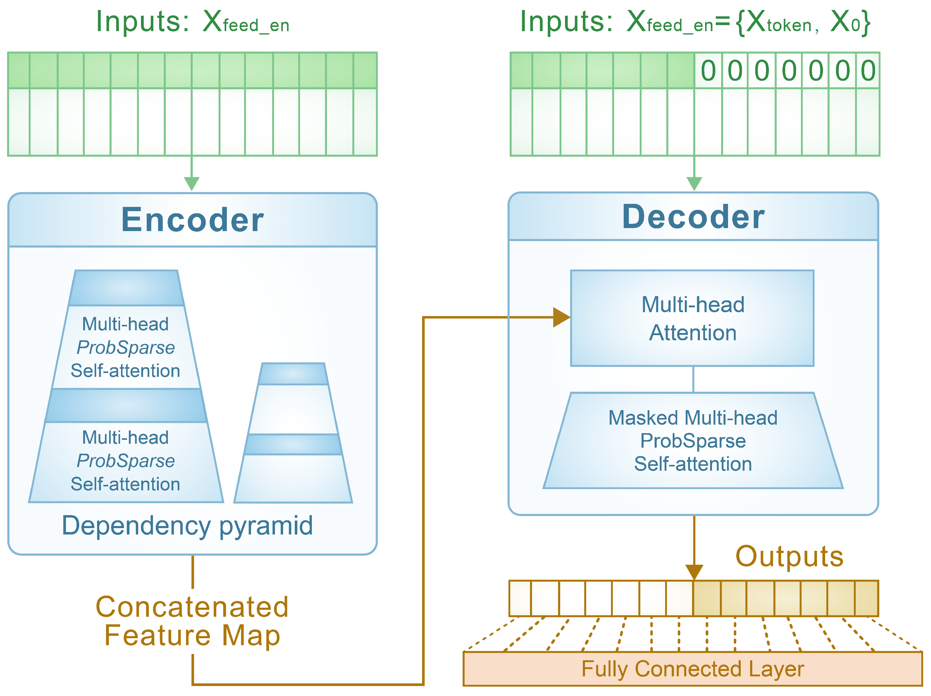
2.4.2. Encoder–Decoder

The encoder first receives the input data and captures the long-sequence dependencies through a dependency pyramid structure. The encoder internally employs a multi-head ProbSparse self-attention mechanism, which reduces computation through probabilistic sparsification while efficiently modeling long-sequence data. The output of the encoder is integrated into a spliced feature map that is passed to the decoder (Figure 3).

The decoder receives the data and utilizes a masked multi-head ProbSparse self-attention layer to ensure that no future information is seen when generating the sequence, which is critical for time-series prediction. In addition, the decoder contains a standard multi-head attention layer to process the feature maps output by the encoder and the decoder’s own output. Finally, the output of the decoder is processed through a fully connected layer to generate the final prediction.

3. VMD–KPCA–xLSTM–Informer Prediction Model

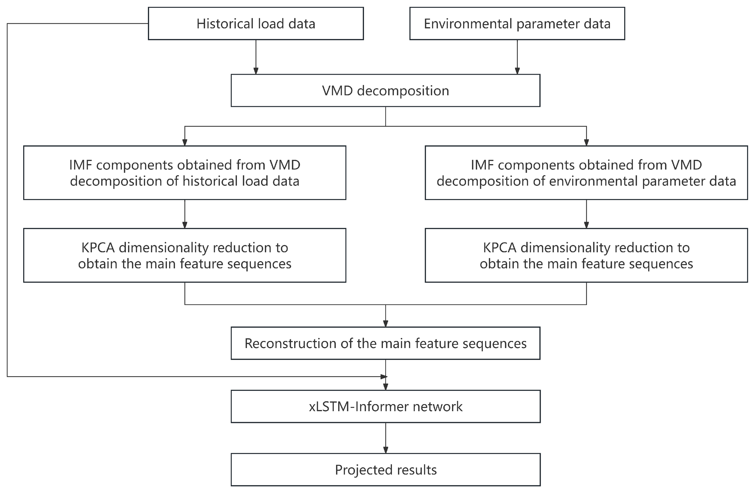
3.1. Construction of the Prediction Model

Electricity load forecasting in this paper is carried out using the VMD–KPCA–xLSTM–Informer model, and the specific model framework structure is shown in Figure 4.

In the VMD decomposition, parameter K is selected according to Equation (9). Historical load data and environmental parameter data are decomposed by VMD to obtain IMF components with different frequencies. Environmental parameters for dataset I include dry bulb temperature, dew point temperature, wet bulb temperature, humidity, and electricity price, and, for dataset II, include temperature. Then, the KPCA algorithm is used to reduce the dimensionality of the IMF components obtained from the decomposition of the historical load data and the environmental parameter data, to facilitate the reduction of the feature dimensions, and the main feature sequences of the historical load data and the environmental parameter data are taken out for reconstruction, respectively. Finally, the downscaled and reconstructed feature sequences are input into the xLSTM–Informer network to obtain the prediction results.

Combining xLSTM and Informer in a cascade for power load forecasting can fully utilize the advantages of both approaches and significantly improve the forecasting performance. xLSTM is good at capturing local time-series features in power load data, especially short- and medium-term complex nonlinear patterns through the extended memory cell and multi-layer gating mechanism, while Informer is based on the Transformer architecture and utilizes the ProbSparse self-attention mechanism to capture global dependencies and efficiently process long-series data. In the cascading process, xLSTM is used to preprocess the input data, and then the processed data are passed to Informer’s encoder and decoder to realize the effective fusion of local time-series features and global dependencies. Experiments show that this combination reduces the model in mean absolute percentage error by 0.65%, and the combination of the two is able to better adapt to the multi-scale characteristics of power load data, including short-term fluctuations, medium-term trends, and long-term periodicity.

In addition, the adaptive time-step mechanism of xLSTM and the ProbSparse attention mechanism of Informer together improve the robustness of the model to noise and outliers and enhance the stability of the prediction. The combination of the two also improves the generalization ability of the model, enabling it to adapt to power load data from different regions and time periods. In the long-series prediction task, the synergy of xLSTM and Informer further enhances the accuracy and efficiency of the prediction.

3.2. Model Evaluation Indicators: MAPE, $R^2$

In this paper, the predictive performance of the model is tested by two widely used metrics: the mean absolute percentage error and the coefficient of determination. MAPE is a measure of predictive accuracy that expresses the average of the absolute value of the difference between the predicted value and the actual value as a percentage of the actual value. MAPE is able to quantify the magnitude of the prediction error, and, because of its percentage form, it allows the easy interpretation and comparison of the predictive performance of different models or different datasets. $R^2$ is a statistical measure of the goodness-of-fit of a model, which reflects how well the model fits the observations: the closer the value is to 1, the better the model is at explaining the correlations. The formulas for calculating MAPE and $R^2$ are as follows:

$$\mathrm{MAPE}={\displaystyle \frac{100\%}{n}}\sum _{i=1}^n\left|{\displaystyle \frac{y_i-{\widehat{y}}_i}{y_i}}\right|$$

(19)

$$R^2=1-{\displaystyle \frac{{\sum }_{i=1}^n{\left(y_i-{\widehat{y}}_i\right)}^2}{{\sum }_{i=1}^n{\left(y_i-\overline{y}\right)}^2}}$$

(20)

where n is the number of samples, $y_i$ is the actual value of the ith sample, ${\widehat{y}}_i$ is the predicted value of the ith sample, and $\overline{y}$ is the average of the actual values. Although MAPE and $R^2$ are widely used in evaluating power load forecasting models, the evaluation results of MAPE and $R^2$ may be distorted and unable to accurately reflect the performance of the model when there are noises, missing values, or outliers in the power load data, which need to be comprehensively evaluated with other indicators.

4. Experimental Results and Analysis

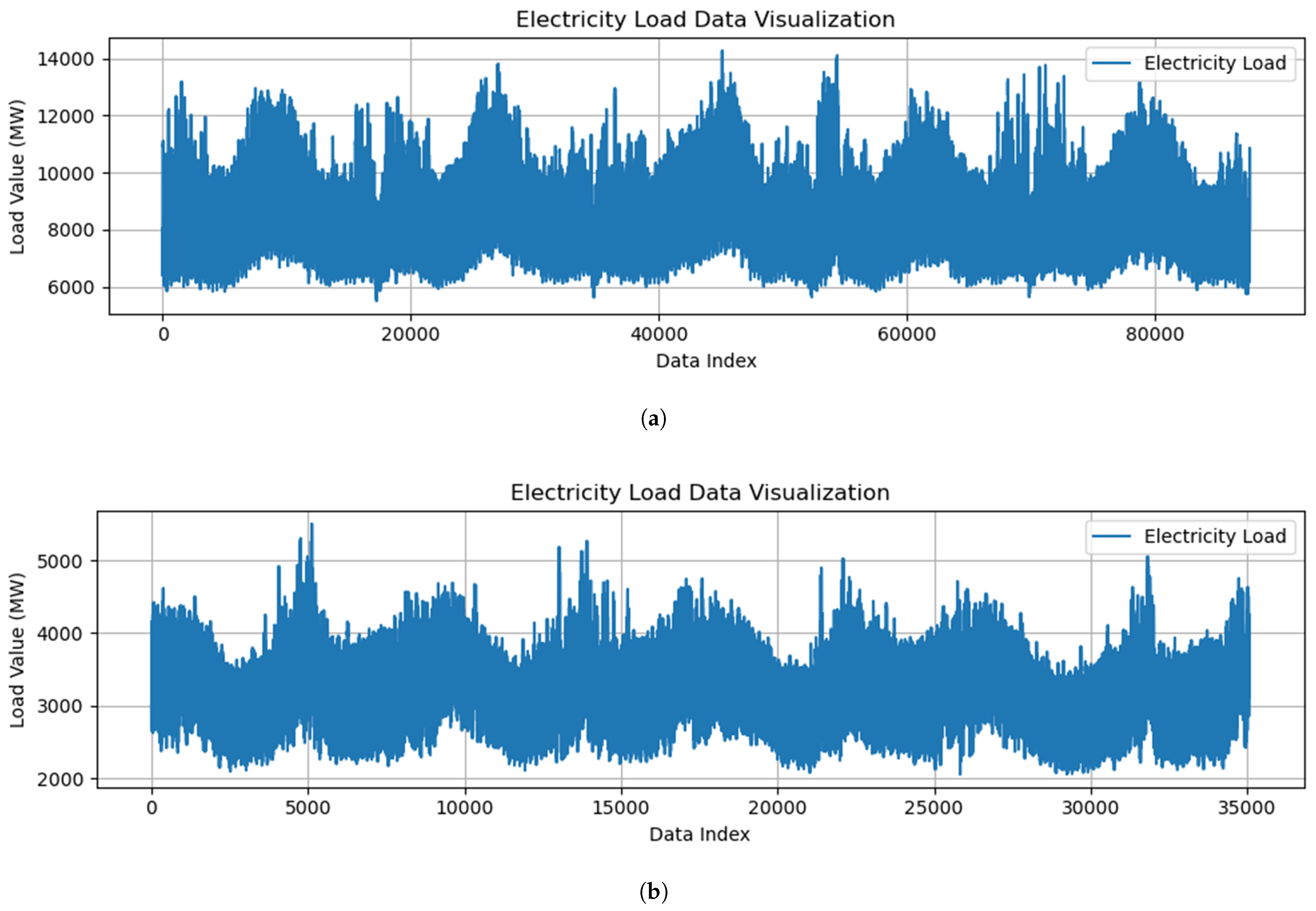
4.1. Datasets and Parameterization

To verify the generalization ability of the model, two datasets are used in this experiment (Figure 5). Dataset I uses measured time-series data of electricity load in an area of Australia and collects environmental information obtained from environmental monitoring devices. The time period of data collection is from 1 January 2006 to 1 January 2011. The environmental information obtained includes five parameters: dry bulb temperature, dew point temperature, wet bulb temperature, humidity, and electricity price. The environmental monitoring device samples the electric load every 30 min for a total length of 87,648. Dataset II is the GEFCom2014 public dataset, which is a standard dataset widely used for electric load forecasting. In this experiment, only the hourly load statistics from 1 January 2006 to 31 December 2009 are selected from the GEFCom2014 dataset, and the environmental information obtained is one parameter, temperature, with a total length of 35,064. When processing the data, the missing values in the dataset are filled in, and the outliers are eliminated, to ensure that the quality of the data has a positive impact on the model training. The dataset is divided into training set and test set according to the ratio of 8:2, in which the training set is the basis of neural network learning, which contains the sample data that the model needs to learn in the training stage. For the observation periods of dataset I and dataset II, the 8:2 division ratio ensures that the test set covers a complete annual cycle, meeting the general requirements for model verification in the industrial sector and the standards for laboratory proficiency testing. With the training set, the model identifies patterns and relationships in the data and adjusts the internal parameters to optimize the prediction or classification performance. The main roles of the test set are to evaluate the model’s performance on new data, provide performance reports, and ensure fair comparisons between different models. The test set provides an understanding of how well the model works in real-world applications. The dataset in this study focuses on load records from a specific Australian region. Its prediction model may better align with this region’s unique temperature fluctuations, industrial activity cycles, and power usage policies. While the current datasets cover five and three complete seasons, respectively, they lack sufficient samples of rare extreme events. This limited coverage could reduce the model’s prediction stability during high-load-fluctuation scenarios. Additionally, the data have constraints in geographical coverage and external variable completeness. Despite these limitations, experimental results on both datasets confirm the model’s superiority. Future work could enhance universality through multi-region joint training and multimodal data fusion. The main model parameters are as follows: the length of the model input sequence is 10, the length of the sequence of the prediction result is 1, the batch size is 8, the proportion of early terminations is 0.2, the number of heads of attention is 8, the number of training iterations is 20, and the initial learning rate is 0.0001. This paper refers to literature reference [1] for the setting of the model parameters. When searching for the optimal value of a parameter, the remaining parameters are held constant, and the following experiments are performed in turn to determine the optimal parameters.

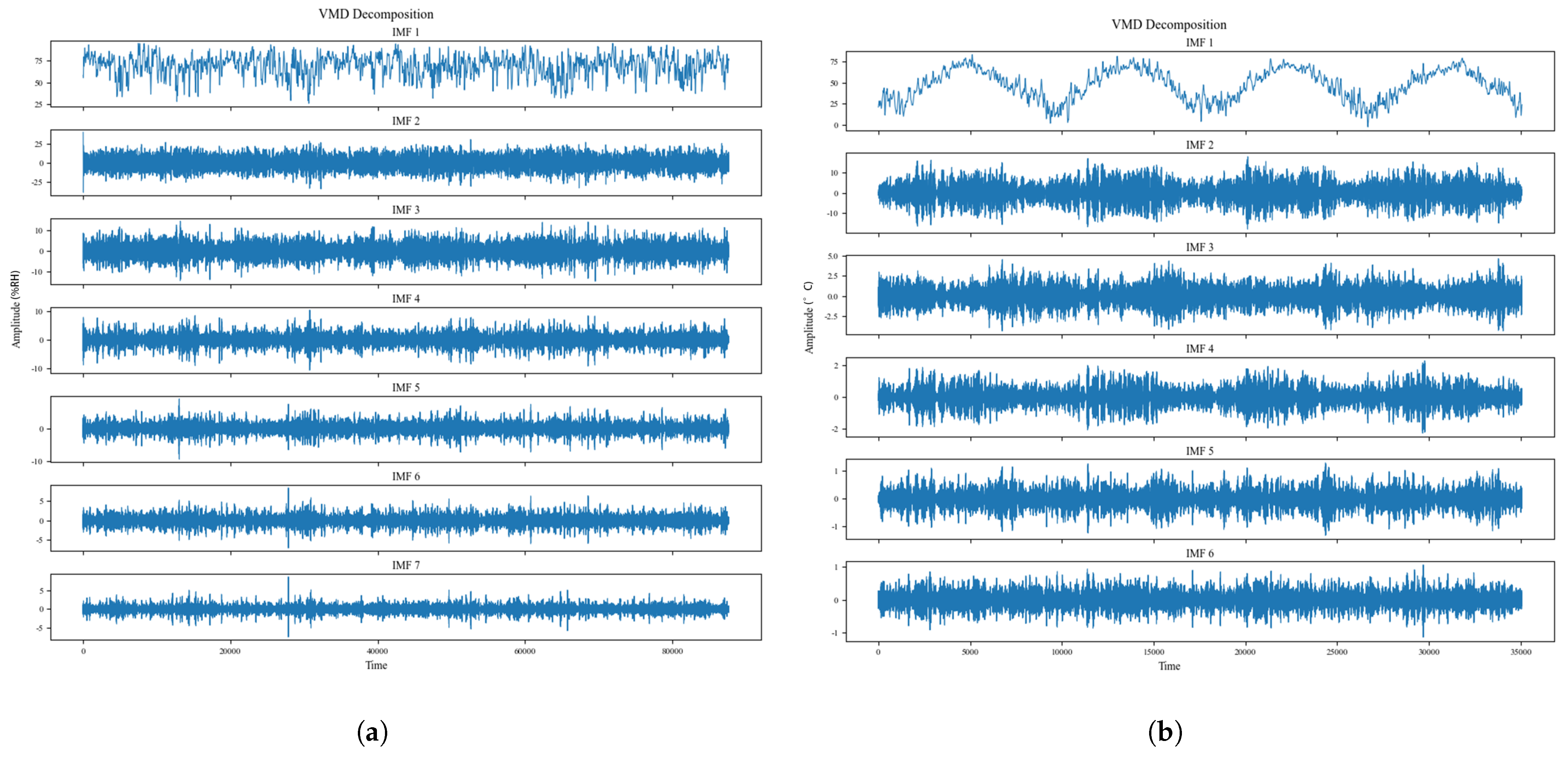
4.2. Variational Mode Decomposition

The historical load data and environmental parameter data are subjected to VMD decomposition. In the VMD algorithm, the quadratic penalty factor $\alpha$ = 2000, the noise tolerance $\tau$ = 0, K is selected by the method of improving the reconstruction error, and the rest of the parameters are default parameters (Figure 6 and Figure 7).

When determining K, the other parameters were kept constant and the reconstruction errors were calculated for different values of K for each piece of environmental parameter data and historical load data, as shown in Figure 6.

Since the data fidelity is higher when the reconstruction error is sufficiently small and there is no significant downward trend, dataset I determines K = 7 as the appropriate number of modals after combining the above six types of data, and dataset II determines K = 6 as the appropriate number of modals after combining the two types of data.

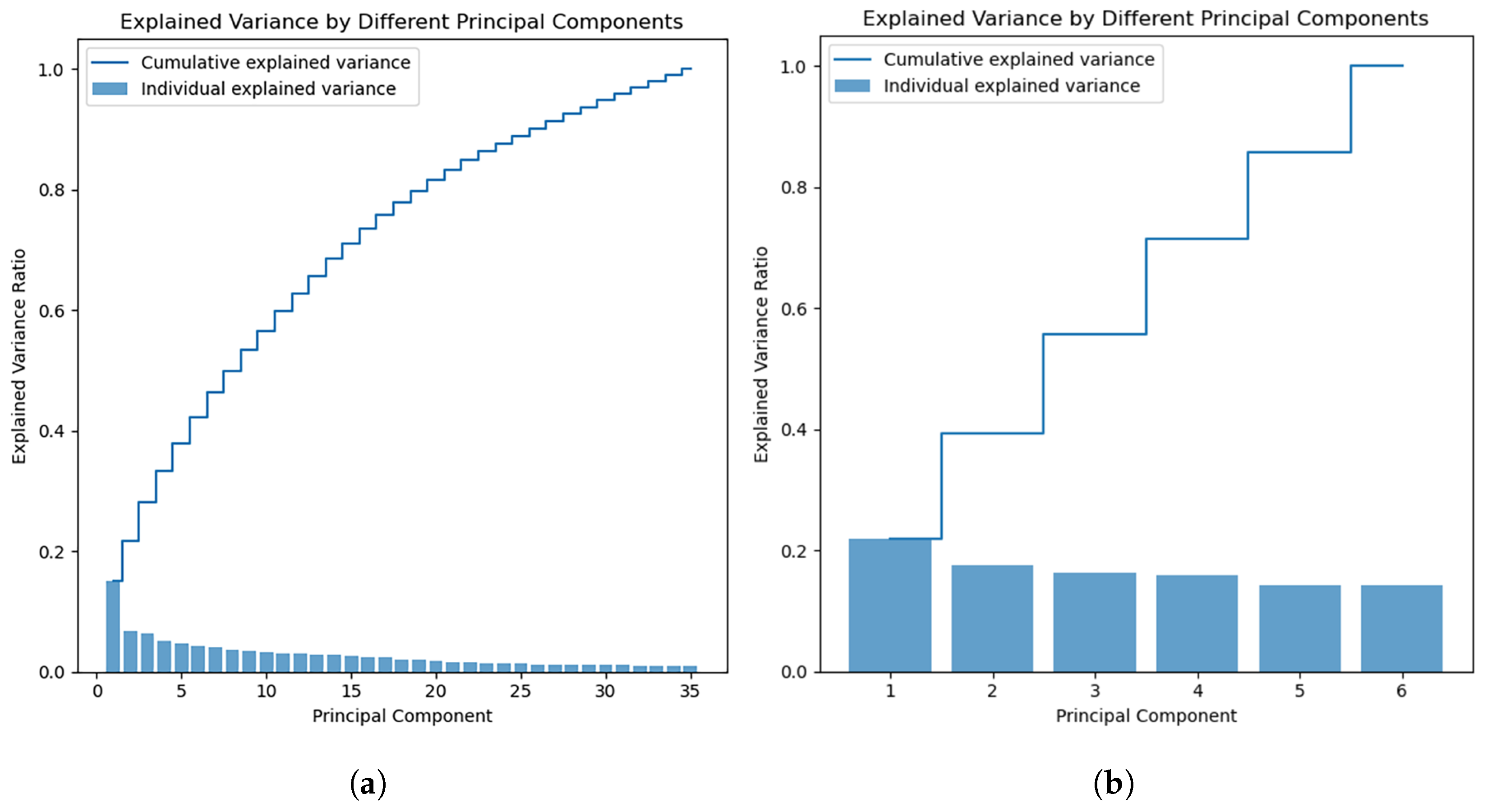
4.3. Kernel Principal Component Analysis

In order to improve the efficiency, accuracy, and generalization ability of the neural network model, this paper uses the kernel principal component analysis algorithm to process the components of the historical load data and environmental parameter data. KPCA sorts the decomposed environmental feature sequences and the historical data sequences of the modes and extracts the sequences with high contribution rate as the input eigenvectors, so that the computational complexity is reduced while retaining the key information to the maximum extent, which is a good foundation for improving the prediction accuracy. As shown in Figure 8 and Figure 9, the top-two components are taken out and reconstructed as input feature sequences.

4.4. Analysis of Experimental Results

4.4.1. Comparison of Different Inputs

In order to verify that the prediction results are better when both historical load data and environmental parameter data are considered, the input feature sequences are set as the sequences with the top-four contribution rates in the historical load data component, the sequences with the top-four contribution rates in the environmental parameter data component, and the reconstructed sequences with the top-two contribution rates of the historical load data component and the environmental parameter data component. They are fed into the xLSTM–Informer model to conduct comparison experiments under the same conditions; the experimental results are shown in

Table 1. Comparative experiments with different input data.

Input Data	Dataset I		Dataset II
	MAPE/%	R2	MAPE/%	R2
Environmental parameters data only	6.562	0.7037	11.064	0.4908
Historical load data only	4.743	0.8553	8.944	0.6720
Combined historical load data and environmental parameters data	2.432	0.9532	4.940	0.8897

.

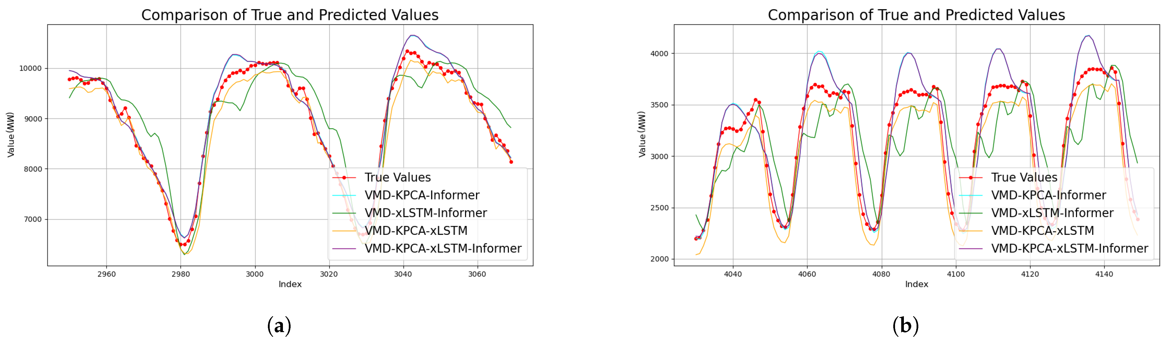
4.4.2. Comparison of Self-Module Prediction Results

In order to verify the reasonableness of the proposed model, the model in this paper is compared with the VMD–xLSTM–Informer, VMD–KPCA–xLSTM, and VMD–KPCA–Informer models under the same conditions in the comparison experiments; the experimental results are shown in

Table 2. Comparative experiments between our own models.

Predictive Model	I Dataset		II Dataset
	MAPE/%	R2	MAPE/%	R2
VMD–xLSTM–Informer	4.357	0.8774	9.013	0.6719
VMD–KPCA–xLSTM	2.518	0.9519	6.173	0.8366
VMD–KPCA–Informer	2.448	0.9531	5.326	0.8657
VMD–KPCA–xLSTM–Informer	2.432	0.9532	4.940	0.8897

. By comparison, the inclusion of modules in this paper’s study improves the prediction accuracy with the lowest mean absolute percentage error on dataset I and dataset II, and the coefficient of determination is closest to 1. Compared with VMD–xLSTM–Informer, VMD–KPCA–xLSTM, VMD–KPCA–Informer, the MAPE metric of this paper’s model is reduced by 44.18%, 3.42%, and 0.65%, respectively, and the $R^2$ metric is improved by 8.64%, 0.14%, and 0.01%, respectively; on dataset II, the MAPE metric of this paper’s model is reduced by 45.19%, 19.97%, and 7.25%, respectively, and the $R^2$ metric is improved by 32.42%, 6.35%, and 2.77%, respectively. It can be concluded that the preprocessing step of performing kernel principal component analysis can effectively extract the key features, reduce the noise interference, improve the model robustness, and play a major role in improving the model accuracy; the combination of xLSTM local temporal modeling and Informer global dependency analysis significantly improves the ability of capturing complex temporal patterns.

Figure 10 shows the experimental results for 120 sample points and visualizes and compares the prediction results of different modules. As can be seen in Figure 10, the data preprocessed by kernel principal component analysis is able to more accurately fit the trend of electricity load data when it rises and falls significantly. However, when the power load data fluctuates at a high frequency, it is difficult for the Informer network to accurately capture these rapidly changing trends. In contrast, xLSTM shows better adaptability when the data fluctuate a lot and can reflect the fluctuating trends more accurately. By using xLSTM for preprocessing the input data and passing the processed data to Informer’s encoder and decoder, the advantages of both can be fully utilized to improve the accuracy of the prediction. This combined approach effectively utilizes xLSTM’s adaptability to multi-scale characteristics and Informer’s ability to model long-term dependencies, significantly improving the overall performance of the model.

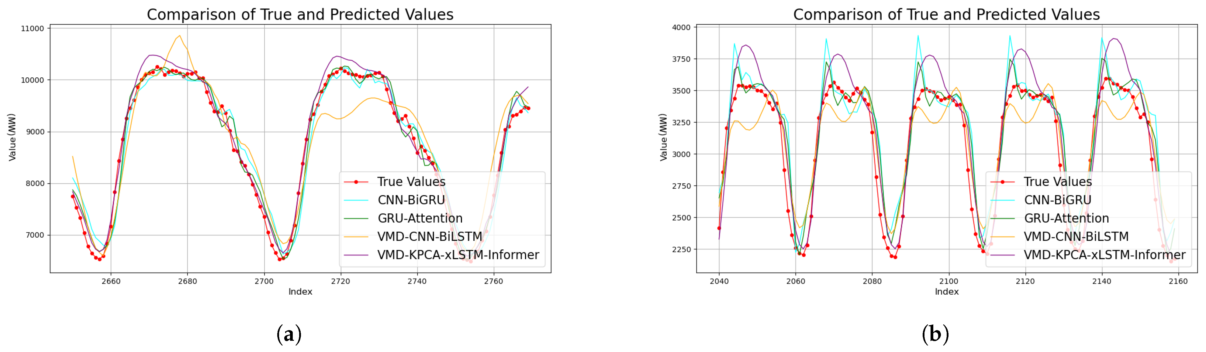
4.4.3. Comparison of Different Model Prediction Results

In order to verify the superiority of the proposed model, the model of this paper is compared with VMD–CNN–BiLSTM [26], CNN–BiGRU [27], and GRU–Attention [28] models under the same conditions in the experimental experiments, and the experimental results are shown in

Table 3. Comparative experiments with different models.

Predictive Model	I Dataset		II Dataset
	MAPE/%	R2	MAPE/%	R2
VMD–CNN–BiLSTM	5.477	0.7750	5.631	0.7882
CNN–BiGRU	3.195	0.9227	5.851	0.7818
GRU–Attention	2.532	0.9487	5.102	0.8416
VMD–KPCA–xLSTM–Informer	2.432	0.9532	4.940	0.8897

. The experimental results show that the VMD–KPCA–xLSTM–Informer model has the lowest mean absolute percentage error on dataset I and dataset II and the coefficient of determination is the closest to 1 when compared to the other three prediction methods. Compared to the VMD–CNN–BiLSTM, CNN–BiGRU, GRU–Attention. This paper’s model reduces the MAPE by 55.60%, 23.88%, 3.95%, and improves the $R^2$ by 22.99%, 3.31%, 0.47%, respectively on dataset I; and, on dataset II, it reduces the MAPE by 12.27%, 15.57%, and 3.18%, and improves the $R^2$ by 12.88%, 13.80%, and 5.72%, respectively. Compared with the above prediction methods, the research method in this paper achieves the optimal performance on both datasets.

Figure 11 shows the experimental results for 120 sample points and visualizes the comparison of the prediction results of different modules. It can be seen that GRU–Attention’s prediction value lags significantly behind the true value at the peak of the power load data and when it fluctuates greatly, indicating its limited ability to capture abrupt patterns; CNN–BiGRU deviates significantly when the data fluctuate and rise, suggesting that the local convolution kernel of the CNN has difficulty in modeling the long time-series dependence and does not introduce the dimensionality reduction preprocessing, which leads to noise interference. The xLSTM–Informer network, compared with the CNN–BiLSTM network, can realize the fusion of local and global features and can better fit the trend of power load data when it rises and falls significantly.

5. Conclusions

A power load forecasting model based on VMD–KPCA–xLSTM–Informer is proposed in this paper. Through comparison among different inputs, the prediction results of the self-module, and the prediction results of different models, the following specific advantages are obtained:

(1)

The input data are decomposed using the VMD algorithm. The completeness of decomposition is measured through reconstruction error. This approach reduces data complexity and enhances prediction model performance. In comparisons with publicly available datasets, the proposed method achieves a MAPE reduction of 3.95% on dataset I and 3.18% on dataset II, outperforming the suboptimal GRU–Attention model. Additionally, the $R^2$ metric shows improvements ranging from 0.47% to 13.80%. Notably, the accuracy in capturing sudden load changes is significantly improved. These results demonstrate the effectiveness of VMD decomposition;

(2)

The KPCA algorithm filters out components with high contribution as input, effectively reducing computational complexity in model training. Our proposed VMD–KPCA–xLSTM–Informer architecture achieves industry-leading performance on dataset I, with a MAPE of 2.432% and an $R^2$ score of 0.9532. Through KPCA preprocessing, the feature dimension is compressed by over 60%. This dimensionality reduction accelerates algorithm execution while simultaneously improving prediction accuracy;

(3)

Comparative experiments conducted with a dual dataset demonstrate significantly better predictive performance when combining historical load data and environmental parameter data, compared to using a single source. On dataset II, the integration reduces the MAPE to 4.940%—a 44.8% improvement over single load input. Simultaneously, the R² increases by 32.4% to 0.8897. These results highlight the model’s enhanced adaptability to complex meteorological factors, confirming that environmental parameters provide critical explanatory power for load fluctuations;

(4)

The combined strengths of xLSTM and Informer cascades are effectively leveraged for power load forecasting. These models excel in time-series feature extraction, global dependency modeling, multi-scale adaptation, and robustness, while also enhancing generalization capabilities. On dataset I, the peak load prediction error remains below ±2.5%. This accuracy enables the power grid dispatching system to achieve 72-hour rolling predictions with 95% confidence. Such performance provides reliable technical support for the economic dispatching of the power system.

Although the model in this paper shows better prediction performance compared with other models, the advantage is not significant enough in the case of less data, such as on dataset II, and still needs to be further adapted to fully utilize the advantage of xLSTM in capturing local time-series features in power load data, especially in the short- and medium-term with complex nonlinear patterns. In addition, the model’s adaptability and generalization ability under extreme climate conditions still need more in-depth research. Future research directions will be devoted to improving the model architecture and enhancing its flexibility and adaptability. The research and development of more efficient parameter optimization algorithms will be conducted, aiming to provide more accurate power load forecasting models for the power system field.

References

1. Li, S.; Cai, H. Short-Term Power Load Forecasting Using a VMD-Crossformer Model. Energies 2024, 17, 2773. [Google Scholar] [CrossRef]
2. Wang, C.-C.; Chang, H.-T.; Chien, C.-H. Hybrid LSTM-ARMA Demand-Forecasting Model Based on Error Compensation for Integrated Circuit Tray Manufacturing. Mathematics 2022, 10, 2158. [Google Scholar] [CrossRef]
3. Yin, C.; Liu, K.; Zhang, Q.; Hu, K.; Yang, Z.; Yang, L.; Zhao, N. SARIMA-Based Medium- and Long-Term Load Forecasting. Strateg. Plan. Energy Environ. 2023, 42, 283–306. [Google Scholar] [CrossRef]
4. Jung, A.-H.; Lee, D.-H.; Kim, J.-Y.; Kim, C.K.; Kim, H.-G.; Lee, Y.-S. Regional Photovoltaic Power Forecasting Using Vector Autoregression Model in South Korea. Energies 2022, 15, 7853. [Google Scholar] [CrossRef]
5. Liu, H.; Shi, J. Applying ARMA–GARCH Approaches to Forecasting Short-Term Electricity Prices. Energy Econ. 2013, 37, 152–166. [Google Scholar] [CrossRef]
6. Ali, S.; Bogarra, S.; Riaz, M.N.; Phyo, P.P.; Flynn, D.; Taha, A. From time-series to hybrid models: Advancements in short-term load forecasting embracing smart grid paradigm. Appl. Sci. 2024, 14, 4442. [Google Scholar] [CrossRef]
7. Chauhan, M.; Gupta, S.; Sandhu, M. Short-Term Electric Load Forecasting Using Support Vector Machines. ECS Trans. 2022, 107, 9731–9737. [Google Scholar] [CrossRef]
8. Guo, F.; Li, L.; Wei, C. Short-term load forecasting based on empirical wavelet transform and random forest. Electr. Eng. 2022, 104, 4433–4449. [Google Scholar]
9. Yao, X.; Fu, X.; Zong, C. Short-Term Load Forecasting Method Based on Feature Preference Strategy and LightGBM-XGboost. IEEE Access 2022, 10, 75257–75268. [Google Scholar] [CrossRef]
10. Lu, S.; Xu, Q.; Jiang, C.; Liu, Y.; Kusiak, A. Probabilistic load forecasting with a non-crossing sparse-group Lasso-quantile regression deep neural network. Energy 2022, 242, 122955. [Google Scholar] [CrossRef]
11. Li, K.; Pan, T.; Xu, D. Short-term power load forecasting based on MSCNN-BiGRU-Attention. China Electr. Power 2025, 57, 162–170. [Google Scholar]
12. Qian, Y.; Kong, Y.; Huang, C. Review of power load forecasting. Sichuan Electr. Power Technol. 2023, 46, 37–43. [Google Scholar]
13. Ibrahim, B.; Rabelo, L.; Gutierrez-Franco, E.; Clavijo-Buritica, N. Machine learning for short-term load forecasting in smart grids. Energies 2022, 15, 8079. [Google Scholar] [CrossRef]
14. Ahmad, A.; Javaid, N.; Mateen, A.; Awais, M.; Khan, Z.A. Short-Term Load Forecasting in Smart Grids: An Intelligent Modular Approach. Energies 2019, 12, 164. [Google Scholar] [CrossRef]
15. Zhang, J.; Zhang, Y.; Chen, X.; Shan, O.; Zhang, W. Research on Short Term Power Load Forecasting Based on AHP-K-Means-LSTM Model. Inn. Mong. Electr. Power 2024, 42, 56–63. [Google Scholar]
16. Cui, Y.; Zhu, H.; Wang, Y.; Zhang, L.; Li, Y. Short term power load forecasting method based on CNN-SAEDN-Res. Electr. Power Autom. Equip. 2024, 44, 164–170. [Google Scholar]
17. Han, J.; Zeng, P. Short-term power load forecasting based on hybrid feature extraction and parallel BiLSTM network. Comput. Electr. Eng. 2024, 119, 109631. [Google Scholar] [CrossRef]
18. Beck, M.; Pöppel, K.; Spanring, M.; Auer, A.; Prudnikova, O.; Kopp, M.; Klambauer, G.; Brandstetter, J.; Hochreiter, S. xLSTM: Extended Long Short-Term Memory. arXiv 2024, arXiv:2405.04517. [Google Scholar]
19. Haoyi, Z.; Shanghang, Z.; Jieqi, P.; Shuai, Z.; Jianxin, L.; Hui, X.; Wancai, Z. Informer: Beyond Efficient Transformer for Long Sequence Time-Series Forecasting. In Proceedings of the AAAI Conference on Artificial Intelligence, San Francisco, CA, USA, 2–9 February 2021; pp. 11106–11115. [Google Scholar]
20. Zeng, J.; Su, Z.; Xiao, F.; Liu, J.; Sun, X. Short-term electricity load forecasting based on generative adversarial networks and EMD-ISSA-LSTM. Electron. Meas. Technol. 2024, 47, 92–100. [Google Scholar]
21. Tang, Y.; Cai, H. Short-term electricity load forecasting based on Pyraformer networks. Eng. J. Wuhan Univ. 2023, 56, 1105–1113. [Google Scholar]
22. Yan, Z.; Li, L.; Xu, H.; Zhuang, S.; Zhang, Z.; Rong, Z. Photovoltaic power output prediction based on the white shark algorithm and an improved long short-term memory network. Electr. Gener. Technol. 2025; in press. [Google Scholar]
23. Zhong, Y.; Wang, J.; Song, G.; Wu, B.; Wang, T. Ultra-short-term power load prediction under extreme weather based on secondary reconstruction denoising and BiLSTM. Power Syst. Technol. 2024; in press. [Google Scholar]
24. Ma, H.; Yuan, A.; Wang, B.; Yang, C.; Dong, X.; Chen, L. Review and prospect of load forecasting based on deep learning. High Volt. Eng. 2025; in press. [Google Scholar]
25. Dragomiretskiy, K.; Zosso, D. Variational mode decomposition. IEEE Trans. Signal Process. 2013, 62, 531–544. [Google Scholar] [CrossRef]
26. Tao, P.; Zhao, J.; Liu, X.; Zhang, C.; Zhang, B.; Zhao, S. Grid load forecasting based on hybrid ensemble empirical mode decomposition and CNN–BiLSTM neural network approach. Int. J.-Low-Carbon Technol. 2024, 19, 330–338. [Google Scholar] [CrossRef]
27. Zhang, Y.; Ran, Q.; Shi, Z.; Xiong, R. Considering multi-scale inputs and optimizing the short-term load prediction of CNN-BiGRU. Sci. Technol. Eng. 2024, 24, 14679–14689. [Google Scholar]
28. Gao, K.; Mou, L. A study of time series forecasting based on quadratic decomposition and GRU-attention. Res. Dev. 2023, 42, 80–87. [Google Scholar]
Figure 1. Evolution of the architecture from the traditional LSTM to the improved xLSTM. The left side shows the classic LSTM structure, the core of which is the memory cell regulated by the gating mechanism, which is used for long-term dependency modeling. The middle part optimizes the xLSTM module by introducing parallel processing, enhanced memory capacity, residual connection, and a normalization layer. The right side shows the complete architecture stacked with multiple xLSTM modules, which integrates bidirectional information flow, hierarchical feature extraction, and an attention mechanism to achieve more powerful sequence modeling capabilities.
Energies 18 02240 g001
Figure 2. The handling of queries by the ProbSparse attention mechanism in the Informer network.
Energies 18 02240 g002
Figure 3. The basic architecture of the Informer network, which consists of two parts, the encoder and the decoder, is specifically designed to handle long-sequence time-series prediction problems.
Energies 18 02240 g003
Figure 4. VMD–KPCA–xLSTM–Informer prediction model structure.
Energies 18 02240 g004
Figure 5. Original data: (a) dataset I; (b) dataset II.
Energies 18 02240 g005
Figure 6. Reconstruction error (RE) of known data for different values of K: (a) dataset I; (b) dataset II.
Energies 18 02240 g006
Figure 7. (a) Schematic of the results of the decomposition of humidity data for dataset I; (b) Schematic of the results of the decomposition of temperature data for dataset II.
Energies 18 02240 g007
Figure 8. Schematic representation of the contribution of each historical load data component after KPCA: (a) dataset I; (b) dataset II.
Energies 18 02240 g008
Figure 9. Schematic representation of the contribution of each environmental parameter data component after KPCA: (a) dataset I; (b) dataset II.
Energies 18 02240 g009
Figure 10. Comparison of predicted results between our own models: (a) dataset I; (b) dataset II.
Energies 18 02240 g010
Figure 11. Comparison of predicted results with different models: (a) dataset I; (b) dataset II.
Energies 18 02240 g011