The Global Renewable Energy and Sectoral Electrification (GREaSE) Model for Rapid Energy Transition Scenarios

Abstract

Achieving the Paris Agreement’s 1.5 °C target requires a global-scale energy transition, reaching net-zero emissions by 2050. This transition demands not only a rapid expansion of renewable energy but also significant upfront energy investment, presenting potential trade-offs between near-term energy security and long-term sustainability. Assuming we cannot rely on as yet unproven negative emissions technology, reductions must be achieved directly, requiring fossil fuel phase-out, accelerated electrification, and substantial renewable infrastructure development. This study presents a detailed, transparent methodology for the creation of a simplified global energy system model designed to rapidly evaluate trade-offs between energy and climate policy, integrating energy investment, depletion, and saturation dynamics into energy transition scenarios. The model simulates energy supply and demand across major sectors, accounting for the upfront energy costs of deploying new renewable infrastructure and the dynamics of electrification in different demand sectors. Its transparent, user-controllable framework allows for rapid scenario adjustments based on variables such as population growth, per capita energy demand, rate and extent of electrification, and strength of climate policy. The primary purpose of this paper is to present the system modelling framework. However, we also present preliminary results from scenario analysis that point to two emergent risks: (1) prioritising energy security increases the likelihood of exceeding carbon budgets, while (2) stringent emissions reductions heighten the risk of energy shortages. Even under non-existent climate policy, fossil fuel depletion makes both the renewable transition and electrification of demand inevitable, though delayed transition leads to more severe emissions overshoot. These findings underscore the urgent need for demand reduction strategies and a more nuanced understanding of the energy investment required for decarbonisation. By offering a flexible scenario tool, this study contributes to informed public discourse and policy decisions on balancing energy security, emissions reduction, and climate resilience.

1. Introduction

1.1. Background

Limiting global warming to 1.5 °C above pre-industrial levels, as outlined in the Paris Agreement, requires achieving net-zero carbon dioxide (CO₂) emissions by approximately 2050 [1]. This, in turn, necessitates a rapid, large-scale transition away from fossil fuels towards renewable energy sources. However, such a transition is not merely a question of deploying renewable infrastructure—it also demands substantial energy investment to manufacture, install, and integrate new energy systems [2]. This introduces a fundamental challenge: how much of the global energy supply must be diverted into the task of building the very system needed to sustain future energy demand? Addressing this question is critical for ensuring both energy security and climate change mitigation.

The existing literature has extensively explored pathways to net-zero emissions, primarily through Integrated Assessment Models (IAMs) and scenario-based projections [3]. However, many of these models incorporate negative emissions technologies—particularly Bioenergy with Carbon Capture and Storage (BECCS)—as a key strategy for compensating for continued fossil fuel use [4]. While BECCS and other carbon removal approaches may play a role in long-term climate stabilisation, they introduce significant uncertainties related to land use, technical feasibility/scalability, and energy return on investment (EROI) [4]. If negative emissions technology cannot be relied upon, then the transition to net zero must be achieved through direct emissions reductions, requiring fossil fuel phase-out and electrification of key sectors at an unprecedented pace [5]. This underscores the need to quantify not only the potential of renewable energy but also the energy costs associated with its deployment.

1.2. Energy Transition Scenarios

A crucial gap in the literature concerns the dynamic interactions between energy investment (as in, the investment of energy in the energy transition), demand, and scarcity. Existing scenario models often assume static or exogenous rates of renewable deployment and demand growth, without explicitly modelling how real-world constraints, feedbacks, and trade-offs influence these rates over time. In reality, the energy transition is a highly interdependent process:

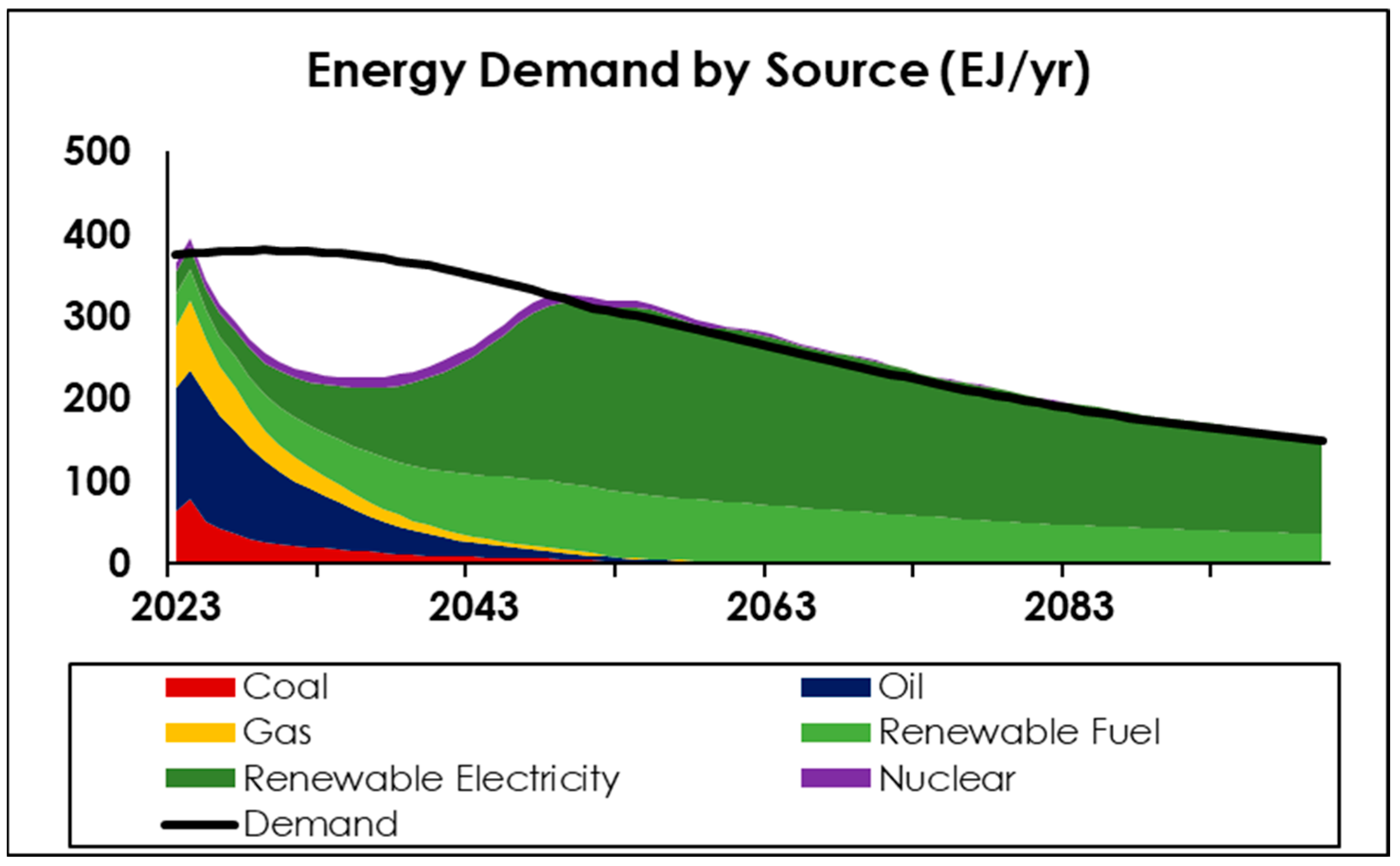
• Fossil fuels remain in the energy mix while renewables are scaled up, but declining fossil fuel availability or policy-driven restrictions on their use can create supply constraints.
• Energy must be diverted from meeting the demand to facilitating the transition itself—building renewable infrastructure requires material extraction, manufacturing, and construction, all of which consume energy.
• Scarcity and energy prices influence investment decisions, affecting both the speed and scale of renewable deployment.
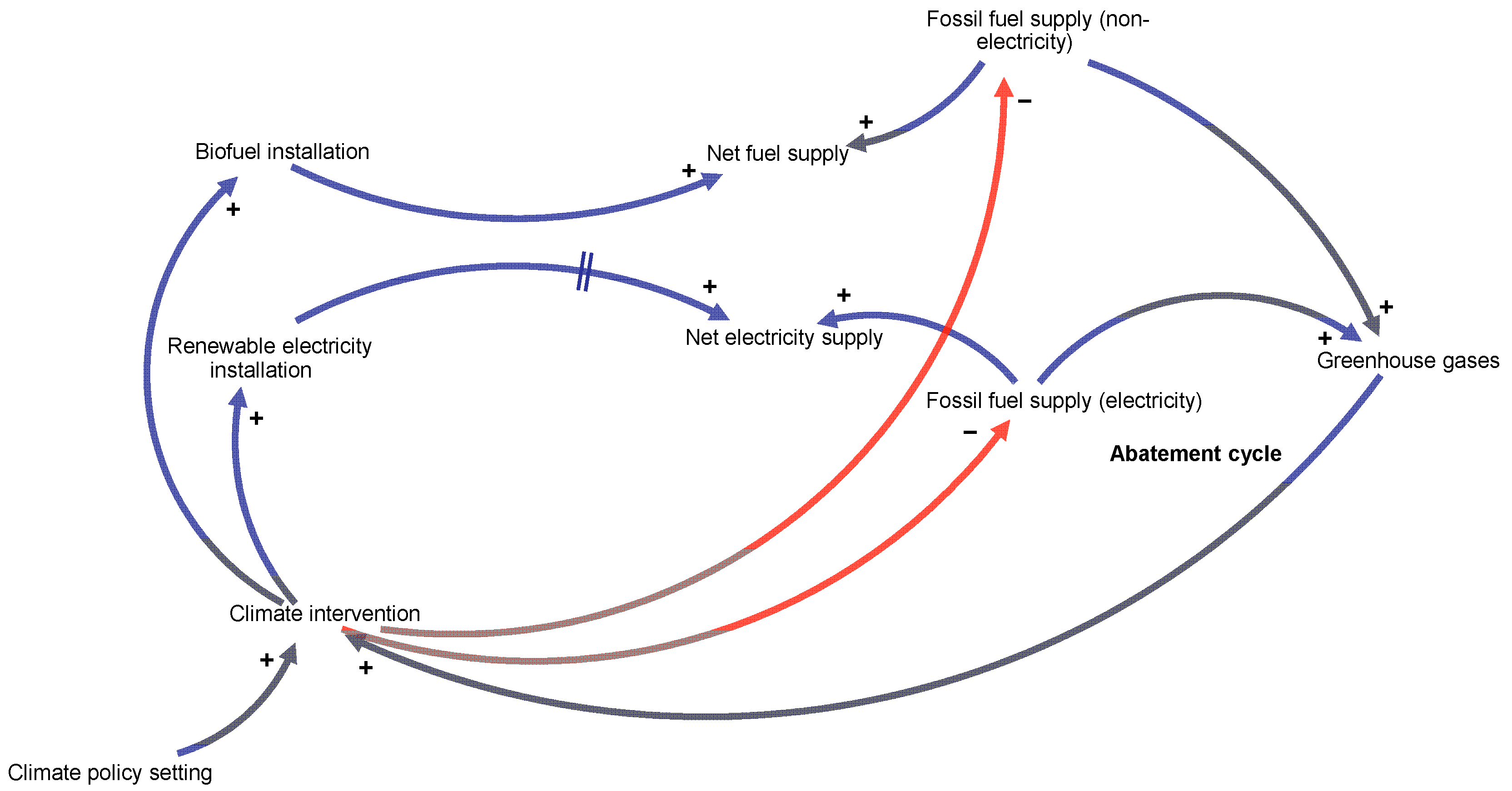
• Climate policy settings shape incentives for investment, demand-side reduction, and fossil fuel phase-out, but the effectiveness of policy depends on how it interacts with these system-level feedbacks.

The concept of energy return on investment (EROI) provides a useful framework for assessing at least some of these trade-offs [6]. Unlike fossil fuels, which require ongoing extraction efforts, renewable energy sources such as solar and wind demand a large initial investment of energy but provide a steady, low-maintenance energy supply over their lifetime [7]. Biofuels, by contrast, require continuous energy input to sustain production and typically exhibit a much lower EROI. These differences have major implications for how quickly and efficiently different renewable pathways can scale up to replace fossil fuels, particularly when accounting for the energy cost of the transition itself.

On the demand side, electrification is widely regarded as the primary mechanism for decarbonising energy consumption [8]. However, the feasibility of rapid electrification varies across sectors. Electricity generation itself is well understood, but major energy-consuming sectors—including transportation and industrial heat—present unique challenges. For example:

• Road and rail transport are relatively straightforward to electrify but require infrastructure upgrades and supply chain adaptations [9].
• Aviation and shipping face significant hurdles, as current battery technologies lack the energy density needed for long-haul applications, making biofuels or synthetic fuels likely alternatives [10].
• Industrial heat processes, particularly in sectors such as steel and cement production, often require extremely high temperatures that are difficult to achieve through direct electrification alone [11].
• Other sectors, including agriculture and residential heating, exhibit varying levels of electrification potential depending on regional resources and policy environments [12,13].

Each of these factors influences the pace and feasibility of the electrification transition, shaping the overall demand for fossil fuels and the associated emissions trajectory. If sectors cannot electrify quickly enough, either (1) demand for biofuels will rise, potentially reaching (or even outstripping) sustainable land use limits, or (2) continued reliance on oil and gas will delay full decarbonisation. Both scenarios present risks: emissions targets may not be met, and fossil fuel depletion could create long-term energy supply challenges. Importantly, the complexity of each sector’s unique electrification challenges means that the spectrum of plausible scenarios is ever-changing, and there is a need for rapid, accessible scenario generation for policymakers and communicators.

1.3. Energy System Models

A plethora of highly sophisticated energy system models are available to generate scenarios that are then available for public use. These include the IEA’s Global Energy and Climate (GEC) Model [14] and Shell’s Global Energy Model [15], and the large family of IAMs used to generate socioeconomic scenarios that underpin climate pathways for the Intergovernmental Panel on Climate Change [3]. However, many existing models and publicly available net-zero transition scenarios tend to ignore, obscure, or downplay the interconnected risks described above. IAMs, while valuable, are often complex, opaque, and inaccessible to non-specialists [16]. Additionally, they may embed rigid assumptions about energy system behaviour, limiting their ability to explore emergent dynamics such as supply shortages, investment bottlenecks, or rapid shifts in policy landscapes [17].

While many scenarios are publicly available, a recurring criticism of the models used to generate them is their lack of transparency. Savvidis et al. [18] explicitly identify this as contributing to a gap between modellers and policymakers, and argue that policymakers should be able to assess a model’s suitability without needing deep technical expertise. Others emphasise the demand for high result reproducibility and transparency for decision-makers [19]. Importantly, the lack of transparency is not limited to proprietary or commercially confidential modelling software; even open access models (OAMs) can lack transparency for individuals without the necessary technical expertise or clear documentation to understand their structure and logic [19]. This effectively creates a situation where even an OAM may function as a ‘black box’ for non-expert users.

The existence of OAMs is, in part, indicative of long-term demand for accessible and transparent energy system analysis tools [19]. Grahn et al.’s GET-RC 6.1 [20] and Bosetti et al.’s WITCH model [21] are examples of models designed explicitly for open access use, but both remain complex and inaccessible to non-expert users. Howells et al. [22] attempted to address this gap by designing their OSeMOSYS model to be ‘Simple, Open, Free and Transportable’ and coupled this with learning resources so that the model can be used to help build understanding of the energy system. While OSeMOSYS is impressive as an educational package and open access research tool, it is not a straightforward scenario generator for immediate use by policymakers.

More recently, researchers have pointed out that even sophisticated models can oversimplify real-world complexities, suggesting that a more transparent, simple modelling approach focusing on the key drivers would offer valuable and complementary insights from a different perspective [23]. In particular, Blondeel et al. suggested that the mainstream modelling approaches do not fully explore scenarios (good or bad) arising from abrupt political shifts, and state that ‘existing inadequacies in these models can constrain the imaginations of energy futures that are brought to the attention of energy policymakers and other relevant stakeholders’ [23]. Adaptive management and planning necessitates a more flexible modelling approach that explicitly incorporates feedback mechanisms between energy supply, demand, and policy choices, while allowing rapid re-assessment of new scenarios as the future continues to evolve.

1.4. Summary

To address this gap, we have developed a simplified model, called GREaSE (Global Renewable Energy and Sectoral Electrification), that enables scenario analysis of plausible pathways for transitioning from fossil fuels to renewables while being simple enough to calculate in a spreadsheet without additional coding. The model integrates the following key system dynamics:

• Existing and future fossil fuel supply, renewable energy deployment, and energy demand;
• Electrification of sectoral energy demand;
• The diversion of energy into building new renewable energy infrastructure, and the implications for net energy availability;
• Supply responses to scarcity and the impact of climate policy settings on the speed and composition of the transition.

By offering a highly controllable, user-friendly scenario tool, with a deliberately parsimonious approach to simulating the dynamics of the energy system, we minimise complexity as a barrier to transparency and understanding. This novel approach enables policymakers, researchers, and stakeholders to test different transition pathways and assess and communicate their implications, while being simple enough to maintain visibility of the key dynamics within the transition.

An important feature of the model is that it explicitly accounts for potential energy constraints (including the depletion of non-renewable resources, saturation of renewable energy, and the energy invested in the renewable transition itself), thereby providing users with the ability to simulate potential risks and trade-offs between emissions reduction, energy security, and transition feasibility. These insights contribute to more informed decision-making by highlighting the complex interplay between climate mitigation, energy system stability, and resource constraints.

2. Materials and Methods

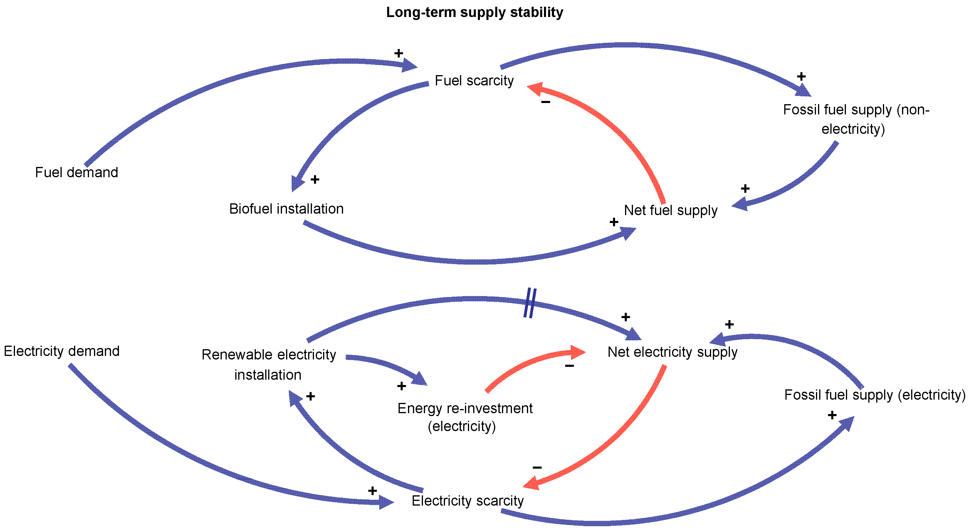
2.1. Conceptual Model

The energy system is first conceptualised using a causal loop diagram (CLD) to represent the key dynamics between supply and demand. The CLD allows a straightforward logic to be applied to take simple cause–effect relationships and progressively build up a sophisticated map of the system (ultimately informing the mathematical model). The software used to generate these CLDs is ‘kumu’ (www.kumu.io, accessed on 25 March 2025).

Following conventional CLD nomenclature, arrow connections flow from cause variables to effect variables. The ‘+’ notation on a connection signifies that change in the effect variable is positively correlated to the cause variable (i.e., increase→increase or decrease→decrease). The ‘−’ notation on a connection signifies an inverse or opposite correlation between cause and effect (i.e., increase→decrease or decrease→increase). By strictly adhering to this logic, loops can be identified as continuously linked cycles of variables connected in the same direction. An odd number of negative connections suggests net stabilising (or oscillatory) behaviour, while either zero or an even number of negative connections creates a reinforcing loop that leads to exponential growth or decay.

To simplify the energy system analysis, supply and demand are each reduced to two main categories: electrical and non-electrical (i.e., fuel) energy. Simplifying the energy system into electricity and fuel allows us to explore the dynamics of the system transformation by simultaneously considering electrification (where demand is initially dominated by non-electric end uses but transitions to a greater fraction of electricity) and the transition towards renewable energy supply, which is dominated by electrical production from resources such as solar and wind.

The drivers of demand in the model are assumed to be, broadly, population growth and economic activity, moderated by efficiency (see Figure 1). This approach is adapted from the Kaya Identity [24] that has historically underpinned climate scenario formulation. For simplicity, the gross domestic product (GDP) per capita and energy intensity of GDP are not explicitly modelled; instead, the model takes a generic ‘per-capita activity’ (effectively the product of these two terms), removing the potential to obfuscate demand for real energy services with additional financial dynamics.

According to this conceptualisation, exogenous variables (external/independent of the model dynamics) are population, per capita activity, and electrification. It is noted that, in the true energy–society system, these variables are not truly exogenous, as feedbacks can occur between population and per capita activity, and both variables (as well as the rate of electrification) could plausibly be influenced by both energy scarcity and climate change. However, as the purpose of this model is to provide a simple, transparent and user-controllable scenario tool, it is deemed sufficient to treat these as quasi-exogenous with the intent that they be used as ‘scenario parameters’ to facilitate testing of hypothetical high-growth versus low-growth demand scenarios, or slow versus rapid electrification.

The model adopts a ‘scarcity’ variable for both fuel and electricity, as shown in Figure 2. Increasing the net supply of energy reduces scarcity (− connection), while increasing demand increases scarcity (+ connection). Scarcity, in turn, promotes energy production, through either the installation of renewable supplies or the extraction of fossil fuels, or both. Note that the ‘scarcity’ variable in this context refers to the short-term supply/demand dynamics, rather than longer-term scarcity caused by the depletion of fossil fuels or reaching the limits of renewable energy potential; those larger processes are included, but are considered separately (detailed below).

The loops between scarcity and supply are negative feedback (odd number of negative connections), meaning that in isolation, these components of the system are self-balancing, i.e., seeking economic equilibrium. This is an intentional simplification of the energy system; a more complete representation would include price (affected by scarcity) with positive connections to supply and negative connections to demand. However, in the interests of keeping the model sufficiently simple to allow user control and build understanding, price dynamics were omitted.

Importantly, the model’s scarcity–supply dynamics account for a key distinction between renewable electricity and all other energy supplies. This distinction is in the form of energy re-investment. It is well established that all energy production requires the investment of energy, which has led to the energy return on investment or EROI concept [25]. However, renewable electricity specifically has the distinction of requiring a large fraction of its energy investment to be made up front, in the building of solar panels, wind turbines, etc., before any energy can be yielded [7]. This is followed by a smaller fraction being invested during operation. Other forms of energy production require comparatively less up-front and more ongoing energy investment.

The distinction between up-front and ongoing energy investment is potentially significant in the context of a major energy system transition, as the roll-out of very large amounts of renewable electricity requires potentially large amounts of energy to be invested in the rapid build-out of the production equipment. The CLD represents this behaviour with two loops: one is the same balancing loop as the other energy scarcity–supply loops (i.e., scarcity leads to more installations of renewable electricity, which increases the net supply and reduces scarcity), while another loop includes the up-front energy re-investment, which (temporarily) reduces net supply. The latter loop is a positive feedback loop (even number of negative connections) meaning it reinforces and could potentially destabilise the system. The stabilising loop ensures that over time, the installed renewable electricity increases the net supply, but the double line on the connection from installation to net electricity supply denotes a delay in this stabilising effect.

Demand and scarcity do not automatically differentiate between renewable versus non-renewable supply. Therefore, in order to capture the dynamics of an imposed transition from fossil fuel to renewable energy, the model requires an exogenous variable representing the ‘strength’ of the climate policy setting. Figure 3 shows the implementation of a simplified climate intervention. Accumulation of greenhouse gases (primarily from burning of fossil fuels) will increase the scale of the required climate intervention. As the required intervention grows, renewable energy supplies should be increasingly preferred over non-renewable fossil fuels. However, we require an exogenous ‘climate policy setting’ variable to govern the magnitude of the actual climate intervention that will be applied. This creates a user-controllable scenario parameter that allows the user to explore the impact of strong versus weak climate policies, while the model remains responsive to demand and scarcity.

In the absence of any carbon emissions policies or targets, we can imagine that fossil fuels might be drawn upon as much as required to satisfy energy demand. However, these non-renewable fuels are themselves finite, and thus eventually the depletion of resources would curtail the ability to grow supplies. Previous research has, for example, explored scenarios of fossil fuel depletion serving as constraints to greenhouse gas emissions [26]. Whilst strong climate policy may lead to a reduction in fossil fuel production before depletion forces these limits, it remains important to include the dynamics in order to test plausible worst-case scenarios with very weak climate policies. Therefore, for completeness, the model includes (simplified) depletion dynamics, implemented as a straightforward negative feedback between a ‘depletion’ variable and the supply, shown in Figure 4.

Renewable supplies are implemented differently from fossil fuels, in that they do not ‘deplete’ in terms of stocks that can run out, but instead can be expected to ‘saturate’ as they reach limits of potential. This is implemented conceptually as a negative feedback on installation: the more renewable energy is installed, the closer the system gets to saturation, which curtails the possibility for additional installation (Figure 5). The maximum scale of the renewable energy resource depends on factors such as the availability of suitable land and water for biofuel production, the availability of physical space for solar and wind, and the availability of water resources for hydropower.

In summary, the conceptual model accounts for (simplified) dynamics between supply and demand and scarcity, facilitating the simulation of growth and decline of renewable and non-renewable sources of fuel and electricity, based on the following user-controllable (exogenous) scenario parameters:

• Population;
• Per capita activity;
• Electrification of demand;
• Climate policy setting.

The dynamics represented in the above conceptual model can be readily translated into a simple numerical model, outlined in the following section and demonstrated through the application of several archetypal scenarios.

2.2. Mathematical Model

2.2.1. Demand

Overall per capita activity at time t is given by A_PC(t), in Joules/person (final energy demand). A_PC is a time series allowing scenarios of static, growing, or shrinking demand to be specified. This is then broken down into n different sectoral demands, A_PC,i, for each sector i such that

$$A_{PC}(t)=\sum _{i=1}^n{A}_{PC,i}\left(t\right)$$

(1)

In the interests of minimising the number of user-specified variables, it is assumed that efficiency improvements (e.g., due to technological innovation) are incorporated into the scenario of A_PC,i. For simplicity we assume that the relative proportions of different sectoral demand (i.e., A_PC,i as a fraction of A_PC) remain static. This is justified on the basis that the intent of the model is to simulate aggregate demand for fuel and electricity, rather than explicitly simulating the dynamic inter-sectoral competition for energy. An alternate formulation could be envisaged that allows re-apportioning of sectoral demands over time, but this is beyond the scope and purpose of the current study.

The model splits each A_PC,i into electric and non-electric (or broadly, fuel) components of demand, according to a time series that represents the electrification scenario:

$${ED}_{PC,i}\left(t\right)=L_i\left(t\right).\left(1-{Eff}_i\left(t\right)\right){.A}_{PC,i}\left(t\right)$$

(2)

$${FD}_{PC,i}\left(t\right)=\left(1-L_i\left(t\right)\right){.A}_{PC,i}\left(t\right)$$

(3)

where ED_PC,i and FD_PC,i are the electrical and fuel demand per capita, respectively, for sector i at time t, L_i is the fraction (from 0 to 1) of sectoral demand i that is in the form of electricity at time t, and Eff_i(t) is the change in final demand resulting from different efficiencies between fuel and electrical energy. For example, if transport was to become 20% more efficient due to electrification, then Eff_transport would move from 0 to 0.2 over the timeframe of electrification. This formulation allows for each sector to follow a distinct user-defined scenario projecting the rate and extent of electrification, as well as accounting for any additional efficiency gains (or losses) that electrification may bring.

Per capita electrical and fuel demand are multiplied by population, P(t), to give the overall global final energy demand by sector, ED_i(t) and FD_i(t), respectively. The above demand-side formulation allows the user to specify different scenarios of demand growth/degrowth, sectoral electrification, and future global population.

2.2.2. Scarcity and Supply Feedbacks

Electricity and fuel scarcity, EC(t) and FC(t), respectively, are taken as a simple difference between demand and supply:

$$EC(t)=\sum _{i=1}^n{ED}_i\left(t\right)-ES(t)$$

(4)

$$FC(t)=\sum _{i=1}^n{FD}_i\left(t\right)-FS(t)$$

(5)

where ES(t) and FS(t) are the total net supply of electricity and fuel, respectively, from all renewable and non-renewable sources.

The overall electricity supply, ES(t), is given by the sum of non-renewable and renewable supplies as follows:

$$ES(t)=\sum _{j=1}^m\left({NR}_j\left(t\right).{NRF}_j\left(t\right).{NRE}_j\right)+\sum _{k=1}^p{RE}_{k,net}\left(t\right)$$

(6)

where NR_j(t) is the production of a non-renewable fuel j, NRF_j(t) is the fraction of that fuel directed to electricity, NRE_j is the efficiency of conversion from primary fuel energy to electrical (assumed to be static, NRE < 1), and RE_k,net(t) is the net energy delivered by a renewable electricity source k. The subscript j denotes a given non-renewable resource (e.g., coal) out of a set of m resources, and the subscript k denotes a renewable electricity source (e.g., solar) out of a set of p sources.

The overall fuel supply, FS(t), is given by the following:

$$FS(t)=\sum _{j=1}^m{NR}_j\left(t\right).\left(1-{NRF}_j\right)+RF(t)$$

(7)

where RF(t) is the production of renewable fuel. For the sake of simplicity, we have adopted a single time series representing global production, but it could potentially be simulated as a set of different regions and/or biomass fuel sub-categories, if desired.

Non-renewable and renewable energy supplies are modelled differently, accounting for the different feedbacks (depletion and saturation, respectively), as outlined in the conceptual model (Figure 4 and Figure 5).

2.2.3. Fossil Fuel Depletion and Renewable Energy Saturation

The supply of non-renewable energy requires a simulation of non-renewable resource production, NR_j, for resource type j. Here, we adapt the ‘resource constrained exponential growth’ model proposed by Ward et al. [26]:

$${NR}_j\left(t\right)=\left(1+r_j\left(t-1\right)\right).{NR}_j\left(t-1\right).\left(1-{\displaystyle \frac{{\int }_0^t{NR}_{j}dt}{{RR}_j}}\right).D_j$$

(8)

where RR_j is the ultimately recoverable resource (production units—e.g., tonnes, barrels) remaining at time 0, r_j is the annual growth rate, and D_j is the energy density (Joules per production unit) for resource type j.

The bracketed term at the end of the equation accounts for the gradual depletion: at early time, this term is very close to 1, but as the cumulative extraction approaches the remaining resource, the term gradually shrinks and curtails growth. In Ward et al.’s formulation, the model was entirely on the supply side, with an exponential growth function simulating deliberately high scenarios of growth with no demand interaction, so as to test hypothetical worst-case emissions limits. We have built on their model to take a time-varying growth rate that allows production to respond dynamically to demand and scarcity (see below).

NR_j can be simulated for as many resources as desired. In this paper, for simplicity we have disaggregated into four global resource supplies (oil, coal, gas, and uranium). It is possible to disaggregate further, e.g., to simulate production at regional, national, or even sub-national levels, and/or model different sub-categories of fuel separately. However, we contend that such a level of detail would produce a misleading level of detail in the dynamics, due to the inability to accurately model the scarcity, demand, and trade/substitution between regions and fuel categories. Refining the model to represent such dynamics may be possible, but is beyond the scope of our rapid scenario tool.

Renewable electricity supply, RE_k(t), is modelled via a three-step calculation, beginning with the amount of electricity of type k built during timestep t, given by RE_k,build:

$${RE}_{k,build}\left(t\right)={RE}_{k,net}\left(t-1\right).r_k\left(t-1\right).\left(1-{\displaystyle \frac{{RE}_{k,installed}(t-1)}{{RE}_{k,max}}}\right)+{\displaystyle \frac{{RE}_{k,installed}(t-1)}{T_k}}$$

(9)

where RE_k,net is the net renewable electricity, r_k is the time-varying growth rate, RE_k,installed is the total installed capacity, RE_k,max is the maximum potential (i.e., saturation) of source type k, and T_k is the average lifespan of the installed plant. The first component of RE_k,build is similar to the formulation of NR_j—i.e., the production increases according to a time-varying growth rate that allows a response to demand and scarcity, and the bracketed term forces the build-out to slow and eventually stop as installed capacity approaches the upper limit. The final component accounts for the need to replenish infrastructure that has reached its end of life.

The installed capacity, RE_k,installed(t), is given by the following:

$${RE}_{k,installed}(t)={RE}_{k,installed}(t-1)+{RE}_{k,build}(t)-{\displaystyle \frac{{RE}_{k,installed}(t-1)}{T_k}}$$

(10)

Put simply, the installed capacity increases by the number of new plants added at each timestep (RE_k,build) and decreases by the number of plants that are retired due to reaching their end of life.

A key part of the conceptual model is the up-front investment of energy required in the build-out of the renewable electricity (Figure 2). For simplicity, this energy investment is assumed to occur entirely during the same timestep as the build and is subtracted from the overall supply to give the net renewable electricity available RE_k,net as follows:

$${RE}_{k,net}(t)=R{E}_{k,installed}(t)-{\displaystyle \frac{{RE}_{k,build}\left(t\right).T_k}{{EROI}_k}}$$

(11)

where EROI_k is the energy return on energy invested for source k. For instance, if EROI_k = 10, then the up-front energy investment (removed from the net supply during this timestep) would equal one-tenth of the lifetime energy of the newly built supply.

In essence, the biofuel model behaves in the same way as the renewable electricity model with a lifespan of one year, replacing RE_k with RF and setting T = 1. This implies the installed biofuel capacity each year, RF_installed(t), can be taken as equal to the capacity ‘built’ that year, RF_build(t), and—assuming a one-year cropping cycle—all capacity is effectively retired and then rebuilt the following year. Adapting Equations (9)–(11) thus gives the following formulation for biofuel:

$${RF}_{build}\left(t\right)={RF}_{net}\left(t-1\right).r_{RF}\left(t-1\right).\left(1-{\displaystyle \frac{{RF}_{build}(t-1)}{{RF}_{max}}}\right)+{RF}_{build}(t-1)$$

(12)

$${RF}_{net}(t)={RF}_{build}(t)-{\displaystyle \frac{{RF}_{build}\left(t\right)}{{EROI}_{RF}}}$$

(13)

where r_RF is the growth rate for biofuel from the previous timestep, RF_max is the saturation potential for biofuel, EROI_RF is the energy return on energy invested for biofuel, and RF_net(t) is the net biofuel energy available to society.

2.2.4. Dynamic Growth Rates

The supply of fossil fuel and renewable energy is modified by a dynamic growth rate that changes depending on a scarcity signal. This is then modified by climate policy. The scarcity signal is derived from the relative scarcity of electricity and fuel, i.e., the absolute scarcity relative to final demand.

For electricity and fuel, respectively, the scarcity signals s_E(t) and s_F(t) are given by the following:

$$s_E(t)={\displaystyle \frac{EC\left(t\right)}{ED\left(t\right)}}$$

(14)

$$s_F(t)={\displaystyle \frac{FC\left(t\right)}{FD\left(t\right)}}$$

(15)

The required climate intervention is defined based on cumulative emissions overshoot relative to the target pathway:

$${CI}_{required}(t)={\displaystyle \frac{{\int }_0^t{GHG}_{model}dt}{{\int }_0^t{GHG}_{target}dt}}$$

(16)

where GHG_model(t) and GHG_target(t) are emissions from the modelled fossil fuel system and the fossil fuel emissions on the target emissions pathway.

GHG_model(t) is calculated as follows:

$${GHG}_{model}(t)=\sum _{j=1}^m\left({NR}_j{\left(t\right)C}_j\right)$$

(17)

where C_j is the carbon intensity of fossil fuel type j.

The extent to which the required climate intervention is actualised is given by CI_actual(t), which is determined by an exogenous ‘climate policy setting’ scenario parameter, CP. This is a number from 0 to 1, where 0 represents no climate intervention and 1 represents the strongest possible intervention.

$${CI}_{actual}\left(t\right)=CP.{CI}_{required}\left(t\right)$$

(18)

The renewable electricity and biofuel growth rates are taken as the sum of relative scarcity and climate intervention as follows:

$$r_k\left(t\right)=s_E\left(t\right)+{CI}_{actual}\left(t\right)$$

(19)

$$r_{RF}\left(t\right)=s_F\left(t\right)+{CI}_{actual}\left(t\right)$$

(20)

For this paper, all renewable electricity sources (k) are assigned the same scarcity-induced growth rate. It is possible to differentiate the growth rates by energy source. For example, a user could assign different weightings to scarcity and climate policy for each source. However, this level of detail is beyond the scope of the paper. The focus here is on generating global scenarios that are simple and fast to produce.

Fossil fuel production is assumed to be versatile and able to meet either electricity or fuel demands via the dynamic NRF_j(t) term. This term evolves over time in response to the changing relative scarcities of electricity and fuel as follows:

$${NRF}_j\left(t\right)={NRF}_j\left(t-1\right).\left(1+s_E(t-1)-s_F(t-1)\right)$$

(21)

Importantly, this allows the energy system—including the fossil fuel supply—to respond to the electrification scenario, independent of climate policy settings.

The growth rates for fossil fuel production, r_j(t), are constructed to reflect both s_E(t) and s_F(t), as well as CI_actual(t). The target growth rate for non-renewable electricity, r_E,NR(t), and fuel, r_F,NR(t) is calculated as follows:

$$r_{E,NR}\left(t\right)=s_E\left(t\right).\left(1-{CI}_{actual}\left(t\right)\right)-{CI}_{actual}\left(t\right)$$

(22)

$$r_{F,NR}\left(t\right)=s_F\left(t\right).\left(1-{CI}_{actual}\left(t\right)\right)-{CI}_{actual}\left(t\right)$$

(23)

Finally, the growth rates for each fossil fuel type can be determined based on weighting the demands by the fraction of each fuel type being used for electricity:

$$r_j\left(t\right)={NRF}_j\left(t\right).r_{E,NR}\left(t\right)+\left(1-{NRF}_j\right).r_{F,NR}\left(t\right)$$

(24)

2.2.5. Nuclear-Fuelled Electricity

Electricity derived from nuclear energy is assumed to be emissions-free but is derived from a non-renewable fuel. As such, the production is modelled using Equation (7) (same as other non-renewable fuels), but the growth rate (r_j) is determined by Equation (19). This allows the model to dynamically grow nuclear-fuelled electricity, just like renewable electricity. As such, the growth responds to electricity scarcity and/or climate interventions. However, nuclear electricity production is still bounded by the same limits as other non-renewable resources.

2.2.6. Method Summary

The preceding calculation steps describe a deliberately simple numerical modelling process. This process simulates how an energy system changes over time. The changes are driven by user-controlled scenarios, such as population growth, per capita energy demand, electrification, and climate policy interventions. The model is simple enough to be run in a spreadsheet, using a one-year timestep. Even with its simplicity, the model can simulate dynamic interactions. These include how fossil fuel and renewable energy deployment respond to fuel or electricity scarcity, as well as greenhouse gas emissions.

3. Scenario Parameters

In order to demonstrate the application of the model in rapid scenario assessment, we parameterise and run the simulation (implemented in MS Excel) using a set of archetypal scenarios outlined below.

3.1. Static Parameters

Table 1, Table 2, Table 3, Table 4 and Table 5 outline modelling parameters, which—for the purposes of this study—were taken to be constant across all scenarios. Of course, any of these static values could also be varied, allowing additional scenarios to be tested; for example, one could explore the sensitivity of results to larger or smaller values for the maximum renewable energy potential by varying RE_k,max over a range.

Sectoral energy demand can be broken down in multiple ways, with subjective definitions of what is implied by ‘sector’. For the purposes of this analysis, we adopt the demand categories used in publicly available data from the International Energy Agency (IEA) [27], shown in Table 1. These categories are chosen for our modelling because the IEA provides the final demand in terms of both overall energy (A_PC,i) and electricity, which allows us to estimate the extent of the electrification of each sector (L_i). A nominal efficiency gain of 20% is assumed across all sectors except transport, which is assumed to have a greater gain (50%) through electrification. The reason for assuming a larger efficiency gain in transport reflects the efficiency of conversion of the energy provided to the vehicle (A_PC,i delivered as either fuel or electricity) into motion, with very different efficiencies in fuel-burning engines compared to electric motors. Determining the precise level of efficiency gain possible through the electrification of transport and other sectors is beyond the scope of this scenario demonstration, but the model is built in such a way to allow different efficiency scenarios to be tested.

Table 1. Sectoral demand profiles.

Demand Sector, i	Share of Per Capita Activity, APC,i/APC (%)	Initial Proportion Electric, Li (t = 0)	Efficiency Gain from Electrification, Effi
Industry	33.7%	29%	20%
Transport	30.8%	1%	50%
Residential	22.5%	28%	20%
Commercial and Public Services	8.8%	53%	20%
Agriculture/ Forestry	2.4%	31%	20%
Fishing	0.1%	11%	20%
Other Non-specified	1.7%	62%	20%

Table 1. Sectoral demand profiles.

Demand Sector, i	Share of Per Capita Activity, APC,i/APC (%)	Initial Proportion Electric, Li (t = 0)	Efficiency Gain from Electrification, Effi
Industry	33.7%	29%	20%
Transport	30.8%	1%	50%
Residential	22.5%	28%	20%
Commercial and Public Services	8.8%	53%	20%
Agriculture/ Forestry	2.4%	31%	20%
Fishing	0.1%	11%	20%
Other Non-specified	1.7%	62%	20%

Table 2 gives the input parameters for fossil fuel and nuclear sources. Initial production rates, fractions diverted to electricity, and the efficiency of conversion are derived from publicly available data from [27] as follows:

• Initial production rate (NR_j) is taken as ‘total energy supply’ minus the quantities allocated to ‘non-energy use’ within ‘total final consumption’ for each source.
• Fraction to electricity (NRF_j) for coal and gas are each taken as ‘total energy supply’ minus ‘total final consumption’ minus ‘non-energy use’, divided by NR_j.
• Efficiency of electricity conversion (NRE_j) is taken as ‘electricity generation’ divided by (NR_j.NRF_j).

The above steps are somewhat approximate, but allow us to obtain—for the purpose of our simplified scenario model—satisfactory estimates of electric fractions and efficiencies for coal and gas, which together account for the vast majority of the world’s electricity and have a large (>50%) proportion of their primary energy diverted to electricity production. For oil, as only a very small fraction is diverted to electricity, the above simple method of apportioning is not suitable. For the purpose of this analysis, NRE_oil is assumed to be equal to the average of NRE_coal and NRE_gas, and NRF_oil is then derived from ‘electricity generation’ for oil from the IEA [27] and the assumed value of NRE_oil.

The remaining resource, RR_j, is taken from the Energy Institute’s Statistical Review of World Energy [28] for reserves of coal, oil, and gas, each converted to an energy resource based on the fuel’s energy content. Carbon intensity values (C_j) of coal, oil, and gas are taken from the GHG Protocol’s [29] emissions factors. For coal, reserves are split into two main resource types (bituminous and lignite/sub-bituminous) by the Energy Institute. The energy reserve (RR_j) represents the total energy content of these combined reserves, while the value of C_j reflects the weighted average of the two emissions factors from the GHG Protocol.

For nuclear electricity, RR_j is derived from figures from the Nuclear Energy Agency [30], in which ‘global identified recoverable resources’ are estimated at 6.1 million tonnes (in the cost category of <USD130/kgU), and current nuclear electricity capacity of 393 GW is fuelled by 60,100 tU/year. This converts to 0.2 PJ per tonne, allowing the identified recoverable resources to be converted to an energy resource. The very small values of NR_nuclear and RR_nuclear (relative to those of other non-renewable energy sources) points to at best only a minor potential contribution from nuclear energy to the global supply.

Table 2. Non-renewable energy parameters.

Model Parameter	Units	Coal	Oil	Gas	Nuclear
Initial fraction diverted to electricity, NRFj (t = 0)	%	82%	7%	61%	100%
Efficiency of electricity conversion, NREj	%	23%	23%	24%	100%
Initial production rate, NRj (t = 0)	EJ/yr	175	159	138	9.7
Remaining resource, RRj	EJ	25,208	9320	6974	1260
Initial growth rate of fossil fuels and nuclear, rj (t = 0)	% p.a.	3%	3%	3%	0%
Carbon intensity of fossil fuels, Cj	MtCO2/EJ	96.3	73.3	56.1	-

Table 2. Non-renewable energy parameters.

Model Parameter	Units	Coal	Oil	Gas	Nuclear
Initial fraction diverted to electricity, NRFj (t = 0)	%	82%	7%	61%	100%
Efficiency of electricity conversion, NREj	%	23%	23%	24%	100%
Initial production rate, NRj (t = 0)	EJ/yr	175	159	138	9.7
Remaining resource, RRj	EJ	25,208	9320	6974	1260
Initial growth rate of fossil fuels and nuclear, rj (t = 0)	% p.a.	3%	3%	3%	0%
Carbon intensity of fossil fuels, Cj	MtCO2/EJ	96.3	73.3	56.1	-

For renewable electricity, the initial supply (RE_k,net) is taken from the IEA [27] for solar, wind, and hydropower. The lifespan is arbitrarily assumed to be 25 years for solar and wind and 75 years for hydro to reflect the differences between the nature of the infrastructure. The EROI_k values are estimates drawn from the ranges for different energy sources provided by Murphy et al. [31].

Saturation potential (RE_k,max) of renewable energy is the source of disagreement and extreme divergence in the literature, with published estimates varying 100-fold [32]. It is not the intent of this paper to resolve such disagreements; rather, we contend that such divergence points to the usefulness of a simplified scenario tool that remains transparent and readily adjustable in light of revised estimates.

For the sake of our illustrative scenario modelling, we adopt arbitrary (but plausible) figures, optimistically assuming future renewable energy has the potential to approximately double current global primary energy from fossil fuels. The assumed figures for RE_k,net in Table 3 are justified as follows:

• Dupont et al. [33] estimates global solar potential to be between 165 and 1089 EJ/yr, depending on the EROI (less energy is available at higher EROI).
• For wind, Bosch et al. [34] estimate 329,600 TWh (1186 EJ/yr), while Dupont et al. [35] estimate between 100 and 700 EJ/yr, depending on EROI (as with solar).
• For hydro, given the specific impacts and long-lived nature of the infrastructure, there is less rapid growth compared with solar and wind. Moriarty and Honnery [36] provide a review of estimates from the literature in the range of 50 to 95 EJ/yr, with a prevalence of values around 50.

Table 3. Renewable electricity parameters.

Model Parameter	Units	Solar	Wind	Hydro
Initial renewable electricity supply, REk,net (t = 0)	EJ/yr	4.7	7.6	16.1
Saturation potential of renewable electricity, REk,max	EJ/yr	200	700	50
Energy return on investment of renewable electricity, EROIk	-	15	20	70
Lifespan of renewable electricity, Tk	yrs	25	25	75

Table 3. Renewable electricity parameters.

Model Parameter	Units	Solar	Wind	Hydro
Initial renewable electricity supply, REk,net (t = 0)	EJ/yr	4.7	7.6	16.1
Saturation potential of renewable electricity, REk,max	EJ/yr	200	700	50
Energy return on investment of renewable electricity, EROIk	-	15	20	70
Lifespan of renewable electricity, Tk	yrs	25	25	75

Biofuel parameters are given in Table 4. The initial supply is from the IEA for the category ‘Biofuels and waste’ (total final consumption) [27]. This is larger than the renewable electricity sources in Table 3, and reflects a combination of traditional biomass, modern biofuels, and energy-from-waste technologies. As with other renewable energy sources, the literature provides a wide range of estimates for saturation potential (RE_RF,max). Haberl et al. [37] reviewed these estimates and concluded a sustainable level to be between 160 and 270 EJ/yr. Murphy et al. [31] provide a range of EROI estimates for different biofuels; from this range, we adopt the value of 2 representing a mid-range estimate for renewable transport fuels.

Table 4. Biofuel parameters.

Model Parameter	Units	Value
Initial biofuel supply, RERF,net (t = 0)	EJ/yr	39.3
Saturation potential of biofuel, RERF,max	EJ/yr	200
Energy return on investment of biofuel, EROIRF	-	2

Table 4. Biofuel parameters.

Model Parameter	Units	Value
Initial biofuel supply, RERF,net (t = 0)	EJ/yr	39.3
Saturation potential of biofuel, RERF,max	EJ/yr	200
Energy return on investment of biofuel, EROIRF	-	2

The target emissions pathway (Table 5) assumes linear decrease in emissions to 50% of present levels by 2030, and then linear decrease to 0% by 2050. This is broadly in line with the accepted range of scenarios for 1.5 °C warming [38]. Note that the emissions in Table 5 are for fossil fuel combustion only; it is assumed—though not guaranteed—that if the nations of the world are collectively following such a decarbonisation pathway for energy, we will collectively adopt an equivalent pathway for the remaining emissions.

Table 5. Target emissions pathway (for 1.5 °C).

	Fossil Fuel Emissions, GHGtarget (t)
Year	Annual (GtCO2/yr)	Cumulative Since 2023 (GtCO2)
2025	28.8	96.0
2030	17.3	198.6
2035	12.5	270.6
2040	7.7	318.6
2045	2.9	342.6
2050	0.0	345.4
2100	0.0	345.4

Table 5. Target emissions pathway (for 1.5 °C).

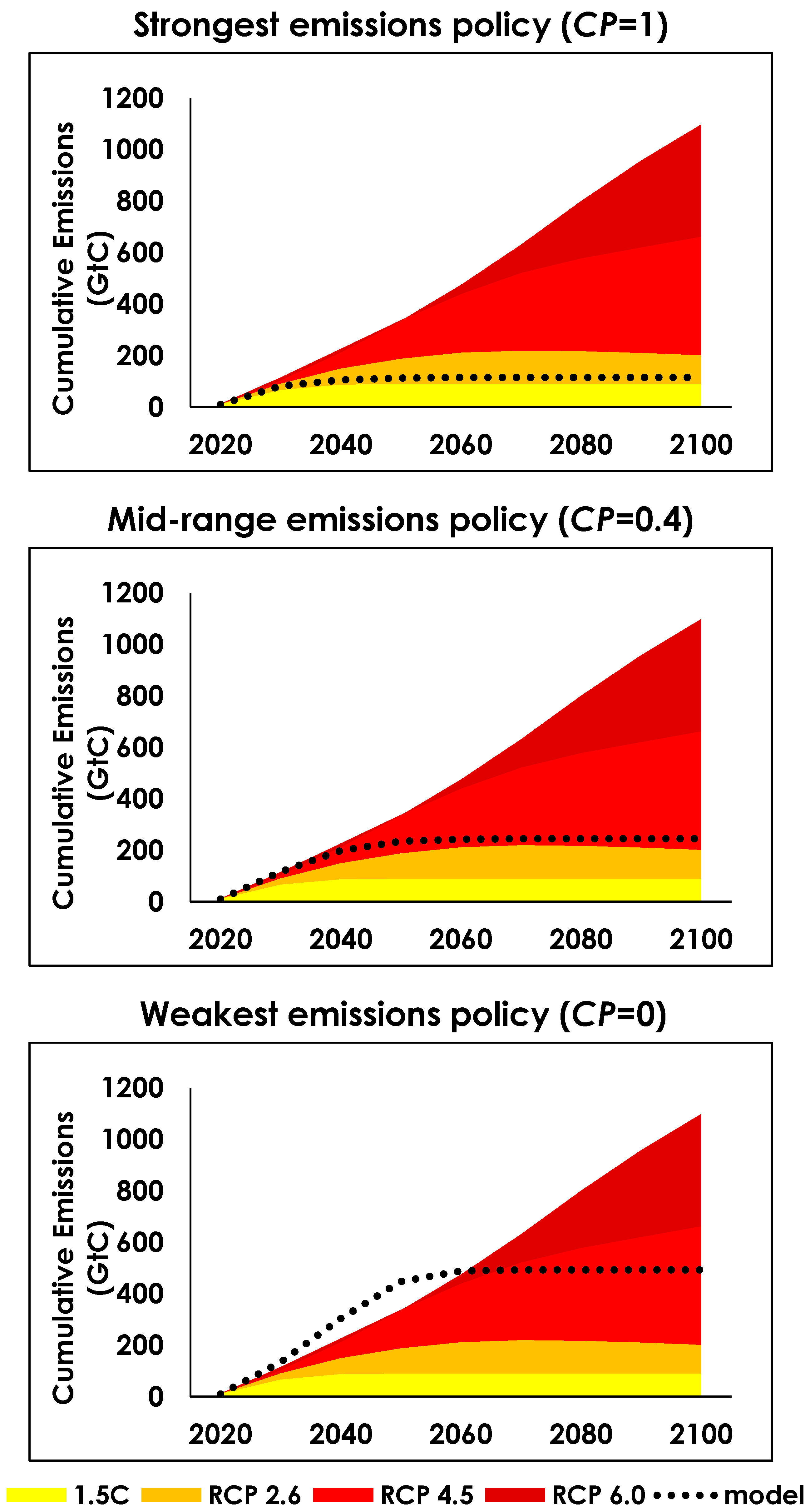
	Fossil Fuel Emissions, GHGtarget (t)
Year	Annual (GtCO2/yr)	Cumulative Since 2023 (GtCO2)
2025	28.8	96.0
2030	17.3	198.6
2035	12.5	270.6
2040	7.7	318.6
2045	2.9	342.6
2050	0.0	345.4
2100	0.0	345.4

3.2. Exogenous Scenario Variables

As noted in relation to the conceptual model development, the model could consider population to be linked (possibly via an inverse relationship) with per capita energy demand, and both could in turn be coupled to energy scarcity (i.e., to allow simulation of a population-energy-poverty trap, and/or scarcity-driven economic shocks). Likewise, the electrification and climate policy settings could also be coupled to energy scarcity and/or per capita demand, to reflect the possibility that a global economy that is deprived of net energy may be less likely to embrace proactive climate action. However, simulating (and validating) the complexity of such linkages is beyond the scope of this study, and these variables are therefore treated as exogenous and under the control of the model user. It is important to note that, when a user of the model specifies a scenario using a particular combination of exogenous scenario variables, they must carefully interrogate the results by taking a critical view of the plausibility of the explicit combination of scenario parameters specified.

For the purpose of this study, three population projections are drawn from the United Nations’ World Population Prospects [39], depicted in Figure 6. These cover a low scenario (peaking at just under 9 billion, around 2050), a medium scenario (peaking around 2080 at just over 10 billion), and a high scenario (increasing approximately linearly to over 14 billion by 2100, without reaching a peak). We refrain from commenting on any likelihood or preference of one population scenario over another, noting that others have done so [40]. It is, however, uncontroversial to observe that the larger the ultimate population, the greater the task in terms of satisfying energy demand, whether from fossil fuels or renewable energy. Moreover, the existence of ultimate limits on sustainable renewable energy (dictated by RE_k,max) means that available energy (per capita) to satisfy demand is inversely proportional to the ultimate population size.

We consider four arbitrary per capita activity scenarios, representing a static scenario (continuing at current global average demand levels), a degrowth scenario (falling to half of current average levels), and two growth scenarios. These are shown in

Table 6. Per capita activity scenarios and illustrative present-day countries.

Scenario	Final Per Capita Activity APC (t = 2100) (GJ/Person/yr)	Similar Present-Day Countries (GJ/Person/yr)
Degrowth (0.5× current)	24.4	Indonesia (23.4) Colombia (24.1) Costa Rica (31.2)
Static (current)	47.7	Thailand (44.1) Brazil (45.7) Argentina (53.9)
Medium growth (1.5× current)	71.0	United Kingdom (66.9) Spain (66.9) Italy (76.0)
High growth (2× current)	94.4	Slovenia (92.9) Germany (94.2) New Zealand (99.4)

and Figure 7. Table 6 has an accompanying list of countries to provide indicative reference energy consumption levels based on present-day demand. In other words, the scenario could represent a transition to a hypothetical world where average activity globally may be similar to that of present-day countries in this list. Current per capita energy demand (globally and for individual countries) is taken from the IEA [27] and is total final consumption minus non-energy use divided by current population from [39].

The sectoral electrification scenarios are given in

Table 7. Assumed ultimate electrification potential (% final demand met by electricity) by sector.

Demand Sector, i	Current Level of Electrification, Li (t = 0)	Maximum Level of Electrification, Li (t)
Industry	29%	up to 100%
Transport	1%	up to 75%
Residential	28%	up to 100%
Commercial and Public Services	53%	up to 100%
Agriculture/Forestry	31%	up to 60%
Fishing	11%	up to 50%
Other Non-specified	62%	up to 75%

. The table lists L_i, the proportion of final demand met by electricity in each sector i. The sectors shown are the main sectors listed by the IEA when analysing total final consumption, and whilst these sectors can be further broken down to more detailed end uses, for the purpose of this study the broad sectors are sufficient.

The transport sector represents the greatest challenge to electrification, representing nearly one-third of per capita energy consumption and being, at present, almost entirely non-electric. The electrification of road and rail transport appears to be progressing, and carries significantly more potential than aviation and shipping. Whilst research and development of electrification in the aviation sector has been undertaken, Zhang et al. [41] states that the additional weight of the electric powertrain and battery energy storage will degrade the aircraft performance, although it is possible that a hybrid electric propulsion system may be developed for shorter aviation trips. With the advancement of battery storage, it is making the shipping industry electrification more viable, although the cost of building/converting is still significantly higher than traditional costs. Furthermore, the additional challenge of how to charge or swap batteries whilst in berth is another significant aspect to overcome. Ensuring reliable and safe long-term operation of vessels becomes a complex problem [42]. Therefore, the likelihood of full electrification of the shipping industry is currently unforeseeable. Although the road transport sector improvements in electrification will assist in offsetting the aviation and shipping sectors, given the very low initial level of electrification, it is not appropriate to assume 100% electrification of transport. As agriculture and fishing are partially dependent on transport (or on-farm vehicles) we assume that these sectors present similar barriers to full electrification.

Industrial energy use broadly encompasses many and various industrial activities that contribute to the demand for fuel and electricity, and covers approximately one-third of total energy consumption. With much of the non-electric energy use being for industrial heat, the industrial sector can be transitioned through a combination of direct substitution (replacing fuel-based heating with electric heating and heat pumps) and process redesign (replacing the need for heat), meaning this sector has the opportunity to transition to a high level of electrification [11].

Household energy consumption includes a substantial use of both natural gas, as well as traditional biofuels and waste, for cooking and heating, although alternative electrical appliances are widely available; electrification of household energy faces primarily economic rather than technical barriers, as is reflected in the United Nations’ Sustainable Development Goal 7 and associated targets [43]. We therefore assume that 100% electrification of households is possible.

The final scenario parameter is the climate policy setting, CP, which ranges from 0 (no intervention) to 1 (full intervention).

4. Results and Discussion

Figure 8 illustrates the impact of the climate policy setting, CP. Here, the fossil fuel emissions are compared against the cumulative target emissions (for 1.5 °C) and several representative concentration pathways (RCP2.6, 4.5, and 6.0) from [3]. The results show that when setting CP = 1 (the strongest setting) the emissions are forced, via the r_j(t) term, to conform to the target pathway, delivering emissions in line with the 1.5 °C target. The weakest setting (CP = 0) results in cumulative emissions in between RCP2.6 and RCP4.5, likely equivalent to approximately 2.5–3 °C warming, although cumulative emissions could temporarily track above RCP6.0 according to the model. With the fossil fuel resource constraints assumed in these scenarios, this represents the worst-case result in terms of emissions and therefore global temperature change. An arbitrary mid-range emissions policy (CP = 0.4) is also included to illustrate the adjustment of policy settings between the two extremes, in this case aligning to RCP2.6 (approximately 2 °C).

The fossil fuel emissions are overwhelming dominated by CP and do not vary greatly between different scenarios of population, per capita activity, or electrification. This is a result of the way the model is formulated in terms of the climate policy setting, noting of course that reducing the complexity of international climate policy to a single number between 0 and 1 is a highly idealised formulation. However, a key benefit of setting up the climate policy model in this way is that it allows a common family of scenarios (e.g., generally weak versus generally strong climate policy) to be used to frame the exploration of energy security under different assumptions about population, per capita activity, and electrification. To that end, these same three climate policy scenario ‘families’ (CP = 0, 0.4, and 1) will be used to frame the exploration of several scenario sets. The purpose of this exploration is not to analyse every possible combination of scenario parameters, but rather to use some exemplar scenarios to test the model and illustrate how it responds to different inputs.

The first scenario family to be explored in this way is the strong climate policy (CP = 1). To generate a ‘base case’ scenario, we assume the medium population growth pathway and static (current) per capita activity. Supposing full and rapid electrification (maximum electrification reached by 2050), the model projects a period of increasing energy shortfall, starting within several years and lasting to around 2050, as shown in Figure 9. The magnitude of the shortfall is on the order of half of the overall demand for energy, caused largely by the rapid phase-out of fossil fuels, but partly by the need to take energy out of the system to help build the replacement renewable infrastructure.

Figure 8. Modelled cumulative fossil fuel emissions versus target and RCP scenarios, for several climate policy settings.

Figure 8. Modelled cumulative fossil fuel emissions versus target and RCP scenarios, for several climate policy settings.

Figure 9. Overall energy demand and supply (scenario: strong climate policy, medium population growth, static per capita activity, rapid and full electrification).

Figure 9. Overall energy demand and supply (scenario: strong climate policy, medium population growth, static per capita activity, rapid and full electrification).

Figure 10 shows an alternative to Figure 9, within the same family of strong climate policy, but with high growth in per capita activity, representing a future world where the equitable level of consumption globally would be akin to that of today’s high-income countries. The same pattern emerges with a slightly longer period of energy shortfall as the system chases a higher ultimate demand target, but it may be feasible to envisage future demand eventually being almost met at this high level by renewable sources. Figure 11 shows another variant within this family, being the lowest growth scenario (low population and degrowth in per capita activity to half of today’s average level). Most interestingly, even this ‘best case’ scenario of degrowth exhibits a similar period of unmet demand, lasting until nearly 2050. This result points to a fundamental issue arising from the energy transition, which is the potentially inescapable shortfall of net energy available for economic activity, relative to even modest scenarios of demand.

Turning to the family of weak climate policy scenarios (CP = 0), Figure 12 shows the equivalent fossil fuel-intensive counterpart to Figure 9. In this case, there is still a period of shortfall extending to after 2050, albeit substantially less pronounced (as a fraction of overall demand) due to the ability—in the absence of climate intervention—to extend the supply of energy from fossil fuels. However, the depletion of fossil fuel, and the associated emergence of inescapable scarcity, dictates a transition to renewable energy over a similar timeframe to that of the strong climate policy. The comparison between Figure 9 and Figure 12 demonstrates a significant trade-off between meeting the 1.5 °C climate target versus mitigating a global shortfall in net energy.

In Figure 13, we explore the potential impact of weak climate policy coupled with no electrification of demand in the scenario of static per capita activity and medium population. In this scenario, we see the model prolonging the extraction of fossil fuels for as long as possible, followed by a long-term divergence between demand and supply as renewable electricity is unable to satisfy the non-electric demand for fuels. This unmet demand is influenced strongly by the assumed saturation potential for biofuels, and other scenarios could be explored with larger amounts of land made available for fuel production (with associated environmental impacts). Just as Figure 12 showed that the need to transition to a fully renewable future is independent of climate policy, the scenario in Figure 13 illustrates that failure to significantly (and rapidly) electrify sectoral demand could result in major energy shortfalls, independent of climate policy.

Figure 14 shows a ‘weak policy’ partner scenario to that shown in Figure 10, for high growth in per capita activity. Again, the transition to renewable energy is driven by the eventual depletion of fossil fuels, but in the meantime the weakening of climate policy allows a larger fraction of demand to be met. While the energy shortfall is lessened, the duration is similar to the strong policy case, with the gap between supply and demand only significantly narrowing after about 2060.

A final scenario is explored in Figure 15. In this case, medium climate policy (CP = 0.4, equivalent emissions to RCP2.6) is coupled to low population growth and medium (1.5×) per capita activity. The result follows a similar trajectory to that of the preceding scenarios, and—as may be expected—the shortfall is not as pronounced as in Figure 9, while being somewhat more than in Figure 12. The purpose of choosing this scenario is not to suggest this is a ‘best case’ or preferred pathway, but rather to demonstrate that there are multiple dimensions to consider, hence justifying the presentation of a simple model that empowers users to control and rapidly explore alternative futures.

The results illustrate that the model produces plausible scenarios that are easy to understand—for instance, stronger climate policy curtails fossil fuel production, less sectoral electrification leads to future shortfalls due to limited biofuel, and so on. The model’s simplicity and speed of use enables energy modelling to be undertaken in a curious and exploratory way: the user can rapidly generate insights around a potential future energy shortfall and/or emissions overshoot by adjusting a very small number of inputs, with or without engaging with the mathematical calculations.

While the inherent simplicity of the model is its defining feature, it is important to recognise the limitations that these simplifying assumptions introduce. These include the following:

• Global aggregation of supply and demand, without consideration of trade within or between countries/regions;
• Division into just two overarching categories of energy use (fuel and electricity);
• Uniform response to general ‘scarcity’ of fuel or electricity, ignoring the potential for some fuels or electricity sources to have a market advantage over others;
• Uniform response by all fossil fuels to climate policy and emissions overshoot;
• No explicit treatment of the energy that must be invested in electrification (e.g., build-out of new industrial plant, electric vehicles, batteries, etc.);
• Excluding negative emissions technologies such as BECCS;
• Lack of constraints or delays imposed by the need for additional electrical storage and/or distribution infrastructure.

To overcome these limitations, users with more technical expertise may choose to engage with a larger number of parameters (such as testing the addition of unconventional fossil fuel resources, disaggregating resources by region, modifying saturation levels for renewable energy, etc.). We anticipate that advanced users may experiment with modifying the calculations themselves (such as introducing dynamic sectoral demand proportions, converting exogenous variables to endogenous to test emergent behaviour, etc.). However, we note that making such changes will introduce substantially greater complexity to the model in the form of additional scenario parameters to test, undermining its power as a deliberately simple tool designed to generate rapid insights.

5. Conclusions

This study aimed to present a simplified, transparent model of the energy transition. We have demonstrated that such a model is possible to produce, while still simulating critical dynamics of the energy system including supply and demand, electrification, and climate interventions. A key feature of the GREaSE model is that it is simple enough to be coded in a spreadsheet, and by minimising the number of parameter inputs, it facilitates rapid exploration and communication of novel scenario combinations by non-experts while retaining full transparency for expert users to control the governing parameters.

Preliminary scenario runs using the model already point to major potential policy trade-offs between (in)tolerable levels of global warming versus (in)tolerable levels of net energy shortages; this trade-off warrants deeper discussion among community and policymakers to inform both public policy as well as community expectations around future consumption growth and affluence. Importantly, the scenarios point to the inevitability of both the rapid electrification of demand and transition to renewable supply, irrespective of climate policy, simply due to the depletion of fossil fuels.

The model illustrates, in a transparent way, the importance of accounting for the energy required to fuel the system transformation, as well as systemic drivers of scarcity (depletion of fossil fuels and saturation of renewable energy sources). Failure to properly anticipate these dynamics could lead to major public backlash against strong climate policies due to energy scarcity and potentially rising costs.

Future iterations of the model could be extended to simulate sub-global dynamics (e.g., regional or national production, consumption and scarcity, and international trade). It is also possible to envisage the introduction of coupled relationships between currently exogenous parameters such as population and per capita demand, enabling the exploration of emergent system behaviour, possibly within a stochastic framework to inform existential risks in the global energy system. However, despite its simplicity (and attendant limitations), we anticipate that the model in its current form could be readily applied in a range of use cases, for example:

• Policymakers updating local climate risk profiles (including adaptive capacity) in light of changes in global climate and/or energy policy;
• Industries and governments building a shared understanding of the role played by sectoral electrification in climate change mitigation;
• Economists exploring the influence and significance of renewable energy saturation potential in meeting future global energy demands, with resultant limits on economic growth;
• Educators guiding non-experts (including students) to raise community-level awareness of the trade-offs and interconnected risks associated with meeting energy demand versus achieving 1.5 °C climate targets.

It is intended that this model will be openly extended, updated, and shared by a community of users to facilitate a ‘grass roots’ study of energy and climate scenarios that ultimately complements the highly sophisticated work of the Integrated Assessment Modelling community.

References

1. Rogelj, J.; Shindell, D.; Jiang, K.; Fifita, S.; Forster, P.; Ginzburg, V.; Handa, C.; Kheshgi, H.; Kobayashi, S.; Kriegler, E.; et al. Mitigation Pathways Compatible with 1.5 °C in the Context of Sustainable Development. In Global Warming of 1.5 °C. An IPCC Special Report on the Impacts of Global Warming of 1.5 °C Above Pre-Industrial Levels and Related Global Greenhouse Gas Emission Pathways, in the Context of Strengthening the Global Response to the Threat of Climate Change, Sustainable Development, and Efforts to Eradicate Poverty; Masson-Delmotte, V., Zhai, P., Pörtner, H.-O., Roberts, D., Skea, J., Shukla, P.R., Pirani, A., Moufouma-Okia, W., Péan, C., Pidcock, R., et al., Eds.; Cambridge University Press: Cambridge, UK; New York, NY, USA, 2022; pp. 93–174. [Google Scholar] [CrossRef]
2. Ram, M.; Bogdanov, D.; Aghahosseini, A.; Oyewo, A.S.; Gulagi, A.; Child, M.; Caldera, U.; Sadovskaia, K.; Farfan, J.; Breyer, C. The role of renewable energy in the global energy transformation. Energy Strategy Rev. 2019, 24, 38–50. [Google Scholar] [CrossRef]
3. Byers, E.; Krey, V.; Kriegler, E.; Riahi, K.; Schaeffer, R.; Kikstra, J.; Lamboll, R.; Nicholls, Z.; Sanstad, M.; Smith, C.; et al. AR6 Scenarios Database Hosted by IIASA, International Institute for Applied Systems Analysis, 2022. Available online: https://doi.org/10.5281/zenodo.5886911 (accessed on 25 March 2025).
4. Murphy, D.J.; McManus, P. The energy return on investment of BECCS: Is BECCS a threat to energy security? Energy Environ. Sci. 2018, 11, 2909–2924. [Google Scholar] [CrossRef]
5. IRENA. World Energy Transitions Outlook 2023: 1.5 °C Pathway. International Renewable Energy Agency, Abu Dhabi. 2023. Available online: https://www.irena.org/publications (accessed on 25 March 2025).
6. Murphy, D.J.; Hall, C.A.; Dale, M.; Cleveland, C. Order from chaos: A preliminary protocol for determining the EROI of fuels. Sustainability 2011, 3, 1888–1907. [Google Scholar] [CrossRef]
7. Capellán-Pérez, I.; De Castro, C.; González, L.J.M. Dynamic Energy Return on Energy Investment (EROI) and material requirements in scenarios of global transition to renewable energies. Energy Strategy Rev. 2019, 26, 100399. [Google Scholar] [CrossRef]
8. Gaur, A.; Balyk, O.; Glynn, J.; Curtis, J.; Daly, H. Low energy demand scenario for feasible deep decarbonisation: Whole energy systems modelling for Ireland. Renew. Sustain. Energy Transit. 2022, 2, 100024. [Google Scholar] [CrossRef]
9. Pulido-Sánchez, D.; Capellán-Pérez, I.; De Castro, C.; Frechoso, F. Material and energy requirements of transport electrification. Energy Environ. Sci. 2022, 15, 4872–4910. [Google Scholar] [CrossRef]
10. Fragkos, P. Decarbonizing the international shipping and aviation sectors. Energies 2022, 15, 9650. [Google Scholar] [CrossRef]
11. Lovegrove, K.; Alexander, D.; Bader, R.; Stephen, E.; Michael, L.; Mojiri, A.; Rutovitz, J.; Hugh, S.; Cameron, S.; Urkalan, K.; et al. Renewable Energy Options for Industrial Process Heat; Australian Renewable Energy Agency (ARENA): Canberra, Australia, 2019. [Google Scholar]
12. Fajardy, M.; Reiner, D.M. Electrification of residential and commercial heating. In Handbook on Electricity Markets; Edward Elgar Publishing: Cheltenham, UK, 2021; pp. 506–539. [Google Scholar]
13. Stakens, J.; Mutule, A.; Lazdins, R. Agriculture electrification, emerging technologies, trends and barriers: A comprehensive literature review. Latv. J. Phys. Tech. Sci. 2023, 60, 18–32. [Google Scholar] [CrossRef]
14. IEA. Global Energy and Climate Model—Documentation; International Energy Agency: Paris, France, 2024. [Google Scholar]
15. Shell. World Energy Model: A View to 2100; Shell International BV: The Hague, Netherlands, 2017. [Google Scholar]
16. Robertson, S. Transparency, trust, and integrated assessment models: An ethical consideration for the Intergovernmental Panel on Climate Change. Wiley Interdiscip. Rev. Clim. Chang. 2021, 12, e679. [Google Scholar] [CrossRef]
17. Pereira, L.; Kuiper, J.J.; Selomane, O.; Aguiar, A.P.D.; Asrar, G.R.; Bennett, E.M.; Biggs, R.; Calvin, K.; Hedden, S.; Hsu, A.; et al. Advancing a toolkit of diverse futures approaches for global environmental assessments. Ecosyst. People 2021, 17, 191–204. [Google Scholar] [CrossRef]
18. Savvidis, G.; Siala, K.; Weissbart, C.; Schmidt, L.; Borggrefe, F.; Kumar, S.; Pittel, K.; Madlener, R.; Hufendiek, K. The gap between energy policy challenges and model capabilities. Energy Policy 2019, 125, 503–520. [Google Scholar] [CrossRef]
19. Oberle, S.; Elsland, R. Are open access models able to assess today’s energy scenarios? Energy Strategy Rev. 2019, 26, 100396. [Google Scholar] [CrossRef]
20. Grahn, M.; Klampfl, E.; Whalen, M.J.; Wallington, T.J.; Lindgren, K. Description of the Global Energy Systems Model GET-RC 6.1; Chalmers University of Technology: Gothenburg, Sweden, 2013. [Google Scholar]
21. Bosetti, V.; Carraro, C.; Galeotti, M.; Massetti, E.; Tavoni, M. A world induced technical change hybrid model. Energy J. 2006, 27 (Suppl. S2), 13–37. [Google Scholar] [CrossRef]
22. Howells, M.; Rogner, H.; Strachan, N.; Heaps, C.; Huntington, H.; Kypreos, S.; Hughes, A.; Silveira, S.; DeCarolis, J.; Bazillian, M.; et al. OSeMOSYS: The open source energy modeling system: An introduction to its ethos, structure and development. Energy Policy 2011, 39, 5850–5870. [Google Scholar] [CrossRef]
23. Blondeel, M.; Price, J.; Bradshaw, M.; Pye, S.; Dodds, P.; Kuzemko, C.; Bridge, G. Global energy scenarios: A geopolitical reality check. Glob. Environ. Chang. 2024, 84, 102781. [Google Scholar] [CrossRef]
24. Yokobori, K.; Kaya, Y. Environment, Energy and Economy: Strategies for Sustainability; Bookwell Publications: Delhi, India, 1999. [Google Scholar]
25. Hall, C.A.S. EROI and Industrial Economies. In Energy Return on Investment; Lecture Notes in Energy; Springer: Cham, Switzerland, 2017; Volume 36. [Google Scholar] [CrossRef]
26. Ward, J.D.; Mohr, S.H.; Myers, B.R.; Nel, W.P. High estimates of supply constrained emissions scenarios for long-term climate risk assessment. Energy Policy 2012, 51, 598–604. [Google Scholar] [CrossRef]
27. IEA. World Energy Statistics and Balances; International Energy Agency: Paris, France, 2024; Available online: https://www.iea.org/data-and-statistics/data-product/world-energy-statistics-and-balances (accessed on 25 March 2025).
28. Energy Institute. Statistical Review of World Energy. 2024. Available online: https://www.energyinst.org/statistical-review/home (accessed on 25 March 2025).
29. GHG Protocol. Emissions Factors, Within Calculation Tools and Guidance. 2024. Available online: https://ghgprotocol.org/calculation-tools-and-guidance (accessed on 25 March 2025).
30. NEA. Uranium 2022: Resources, Production and Demand. Joint Report by the Nuclear Energy Agency and International Atomic Energy Agency; OECD Publishing: Paris, France, 2023. [Google Scholar]
31. Murphy, D.J.; Raugei, M.; Carbajales-Dale, M.; Rubio Estrada, B. Energy return on investment of major energy carriers: Review and harmonization. Sustainability 2022, 14, 7098. [Google Scholar] [CrossRef]
32. Moriarty, P.; Honnery, D. Can renewable energy power the future? Energy Policy 2016, 93, 3–7. [Google Scholar] [CrossRef]
33. Dupont, E.; Koppelaar, R.; Jeanmart, H. Global available solar energy under physical and energy return on investment constraints. Appl. Energy 2020, 257, 113968. [Google Scholar] [CrossRef]
34. Bosch, J.; Staffell, I.; Hawkes, A.D. Temporally explicit and spatially resolved global offshore wind energy potentials. Energy 2018, 163, 766–781. [Google Scholar] [CrossRef]
35. Dupont, E.; Koppelaar, R.; Jeanmart, H. Global available wind energy with physical and energy return on investment constraints. Appl. Energy 2018, 209, 322–338. [Google Scholar] [CrossRef]
36. Moriarty, P.; Honnery, D. What is the global potential for renewable energy? Renew. Sustain. Energy Rev. 2012, 16, 244–252. [Google Scholar] [CrossRef]
37. Haberl, H.; Beringer, T.; Bhattacharya, S.C.; Erb, K.H.; Hoogwijk, M. The global technical potential of bio-energy in 2050 considering sustainability constraints. Curr. Opin. Environ. Sustain. 2010, 2, 394–403. [Google Scholar] [CrossRef] [PubMed]
38. UNEP. Emissions Gap Report 2024; United Nations Environment Programme: Nairobi, Kenya, 2024. [Google Scholar] [CrossRef]
39. United Nations. World Population Prospects: 2024 Revision. United Nations Department of Economic and Social Affairs, Population Division. 2024. Available online: https://population.un.org/wpp/ (accessed on 25 March 2025).
40. O’Sullivan, J.N. Demographic delusions: World population growth is exceeding most projections and jeopardising scenarios for sustainable futures. World 2023, 4, 545–568. [Google Scholar] [CrossRef]
41. Zhang, J.; Roumeliotis, I.; Zolotas, A. Sustainable aviation electrification: A comprehensive review of electric propulsion system architectures, energy management, and control. Sustainability 2022, 14, 5880. [Google Scholar] [CrossRef]
42. Qazi, S.; Venugopal, P.; Rietveld, G.; Soeiro, T.B.; Shipurkar, U.; Grasman, A.; Watson, A.J.; Wheeler, P. Powering maritime: Challenges and prospects in ship electrification. IEEE Electrif. Mag. 2023, 11, 74–87. [Google Scholar] [CrossRef]
43. United Nations. Sustainable Development Goals: Goal 7—Ensure access to Affordable, Reliable, Sustainable and Modern Energy for All. 2025. Available online: https://sdgs.un.org/goals/goal7 (accessed on 25 March 2025).
Figure 1. Demand-side variables in the CLD. (Red: −ve connection, blue: +ve connection).
Energies 18 02205 g001
Figure 2. Supply–demand loops for fuel and electricity. (Red: −ve connection, blue: +ve connection).
Energies 18 02205 g002
Figure 3. Greenhouse gas abatement through climate policy and intervention. (Red: −ve connection, blue: +ve connection).
Energies 18 02205 g003
Figure 4. Fossil fuel depletion cycle (for weak climate policy scenarios). (Red: −ve connection, blue: +ve connection).
Energies 18 02205 g004
Figure 5. Saturation of renewable energy potential. (Red: −ve connection, blue: +ve connection).
Energies 18 02205 g005
Figure 6. Low, medium, and high population scenarios from United Nations [39].
Energies 18 02205 g006
Figure 7. Per capita activity scenarios; historical data from IEA [27].
Energies 18 02205 g007
Figure 10. Overall energy demand and supply (scenario: strong climate policy, medium population growth, 2× per capita activity, rapid and full electrification).
Energies 18 02205 g010
Figure 11. Overall energy demand and supply (scenario: strong climate policy, low population growth, 0.5× per capita activity also known as ‘degrowth’, rapid and full electrification).
Energies 18 02205 g011
Figure 12. Overall energy demand and supply (scenario: weak climate policy, medium population growth, static per capita activity, rapid and full electrification).
Energies 18 02205 g012
Figure 13. Overall energy demand and supply (scenario: weak climate policy, medium population growth, static per capita activity, no electrification).
Energies 18 02205 g013
Figure 14. Overall energy demand and supply (scenario: weak climate policy, medium population growth, 2× per capita activity, rapid and full electrification).
Energies 18 02205 g014
Figure 15. Overall energy demand and supply (scenario: medium climate policy, low population growth, 1.5× per capita activity, rapid and full electrification).
Energies 18 02205 g015