
Investigation of the Computational Framework of Leading-Edge Erosion for Wind Turbine Blades

Abstract
1. Introduction
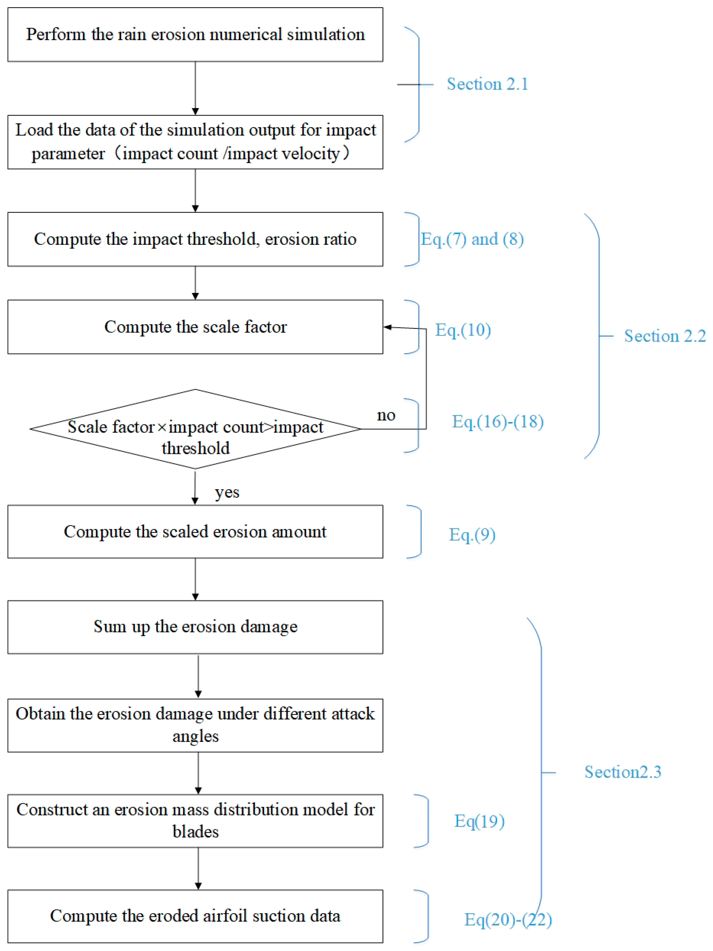
2. Methodology
2.1. Dispersed-Phase Model
2.2. Rain Erosion Degradation Model Based on the Weibull Distribution of the Particle Size
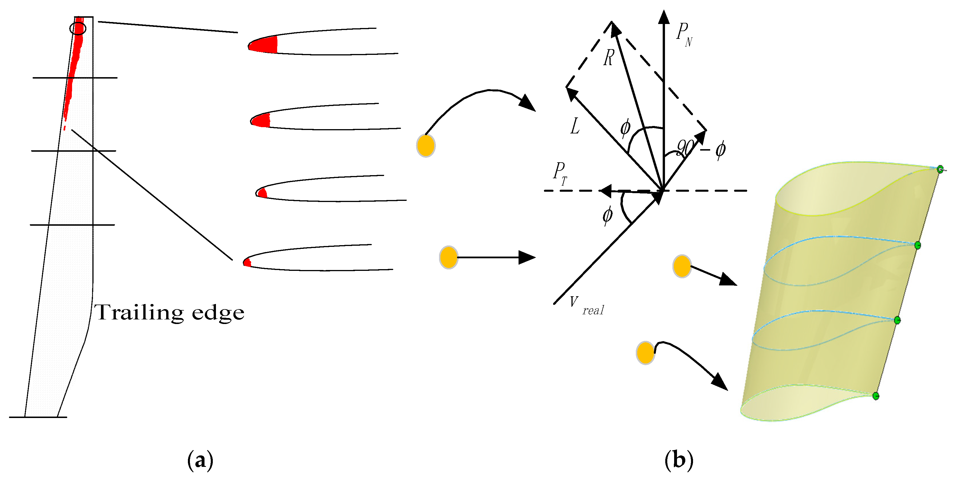
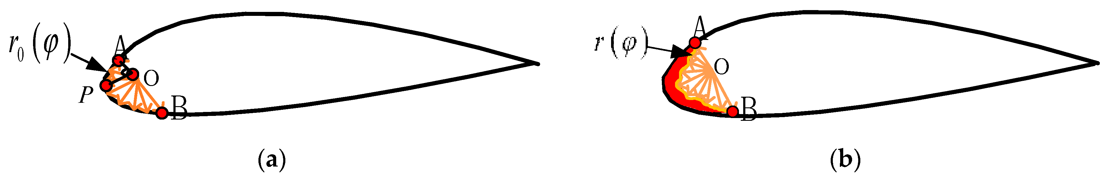
2.3. Three-Dimensional Erosion Computational Model
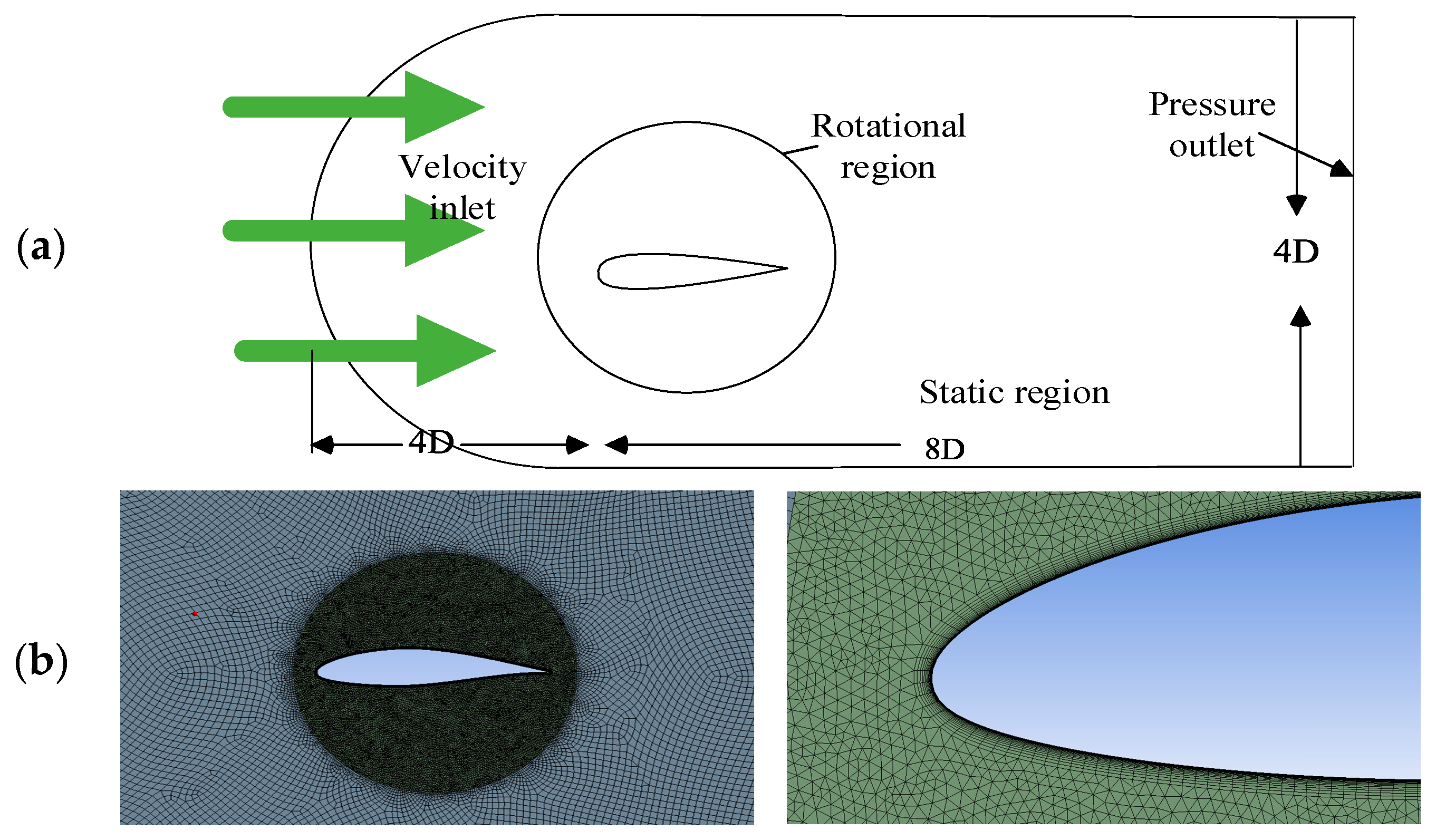
3. Numerical Simulation
4. Result and Discussion
4.1. Erosion Distribution and Validation
4.2. Blade Span Erosion Distribution and Aerodynamic Results
5. Conclusions
Author Contributions
Funding
Data Availability Statement
Conflicts of Interest
Nomenclature
| projected area of the raindrop | initial position of particle cloud | ||
| threshold of impact count | motion time of cloud | ||
| strength of the coating material | velocity of free stream | ||
| stress produced by the raindrop impact | fluid density | ||
| constant parameter | particle density | ||
| constant parameter | gravitational acceleration | ||
| erosion amount | drag coefficient | ||
| erosion amount for each impact | particle diameter | ||
| number of impacting particles | the angle of AO and PO | ||
| mass of droplet | scaling function allocate the necessary erosion mass | ||
| empirical constant | coefficients of sinusoid function | ||
| empirical constant | standard deviation of scaling function | ||
| real erosion mass | variance of scaling function | ||
| scaling factor | constant parameter | ||
| simulation particle number | order of sinusoid function | ||
| total particle number | erosion mass of per unit length of blade | ||
| operating time | density of surface coating | ||
| simulation time | Lagrangian time scale | ||
| inflow velocity | velocity of particle cloud | ||
| simulation time step | particle position | ||
| Weibull distribution function of wind speed | standard deviation of the individual particle position | ||
| rainfall intensity | probability density function | ||
| volume of the droplets | cloud domain | ||
| blade operational velocity | ensemble-averaged quantity | ||
| droplet impact velocity | erosion mass on blade section | ||
| Weibull distribution function of droplet diameter | material density | ||
| constant parameter | constant parameter | ||
| constant parameter | function of attack angle | ||
| real erosion amount | attack angle | ||
| marking variable of erosion occur | clean airfoil curve | ||
| marking variable of current impact count | erosion curve | ||
| jth time step | particle cloud velocity |
References
- Ibrahim, M.; Medraj, E.M. Water droplet erosion of wind turbine blades: Mechanics, testing, modeling and future perspectives. Materials 2020, 13, 157. [Google Scholar] [CrossRef]
- Han, W.; Kim, J.; Kim, B. Effects of contamination and erosion at the leading edge of blade tip airfoils on the annual energy production of wind turbines. Renew. Energy 2017, 115, 817–823. [Google Scholar] [CrossRef]
- Eisenberg, D.; Laustsen, S.; Stege, J. Wind turbine blade coating leading edge rain erosion model: Development and validation. Wind Energy 2018, 21, 942–951. [Google Scholar] [CrossRef]
- Sethi, M.R.; Subba, A.B.; Faisal, M. Fault diagnosis of wind turbine blades with continuous wavelet transform based deep learning model using vibration signal. Eng. Appl. Artif. Intell. 2024, 138, 109372. [Google Scholar] [CrossRef]
- Francisco, J.; José, M.G.; Marcos, O.; Marcelo, G.; Rodrigo, A. A Bayesian approach for fatigue damage diagnosis and prognosis of wind turbine blades. Mech. Syst. Signal Proc. 2022, 174, 109067. [Google Scholar]
- Mielke, A.; Benzon, H.H.; Mcgugan, M. Analysis of damage localization based on acoustic emission data from test of wind turbine blades. Measurement 2024, 231, 114661. [Google Scholar] [CrossRef]
- Wang, Y.; Ma, K.; Peng, Q. Design and performance study of real-time, reliable, and highly accurate carbon fiber reinforced polymer-fiber Bragg grating sensors for wind turbine blade strain monitoring. Opt. Eng. 2024, 63, 037108. [Google Scholar] [CrossRef]
- Li, H.; Wang, Z. Anomaly identification of wind turbine blades based on Mel-Spectrogram Difference feature of aerodynamic noise. Measuremen 2025, 240, 115428. [Google Scholar] [CrossRef]
- Wang, H.Y.; Chen, B. Investigation on aerodynamic noise for leading edge erosion of wind turbine blade. J. Wind Ebg. Ind. Aerod. 2023, 240, 105484. [Google Scholar] [CrossRef]
- Carraro, M.; Vanna, F.D.; Zweiri, F. CFD modeling of wind turbine blades with eroded leading edge. Fluids 2022, 7, 302. [Google Scholar] [CrossRef]
- Papi, F.; Balduzzi, F.; Bianchini, A.; Ferrara, G. Uncertainty quantification on the effects of rain-induced erosion on annual energy production and performance of a multi-MW wind turbine. Renew. Energy 2020, 165, 701–715. [Google Scholar] [CrossRef]
- Maniaci, D.C.; White, E.B.; Wilcox, B.; Langel, C.M.; Van Dam, C.P.; Paquette, J.A. Experimental measurement and CFD model development of thick wind turbine airfoils with leading edge erosion. J. Phys. Conf. 2016, 753, 022013. [Google Scholar] [CrossRef]
- Aird, J.A.; Barthelmie, R.J.; Pryor, S.C. Automated quantification of wind turbine blade leading edge erosion from field images. Energies 2023, 16, 2820. [Google Scholar] [CrossRef]
- Zhang, Y.; Avallone, F.; Watson, S. Leading edge erosion detection for a wind turbine blade using far-field aerodynamic noise. Appl. Acoust. 2023, 207, 109365. [Google Scholar] [CrossRef]
- Wang, Y.; Zheng, X.; Hu, R.; Ping, W. Effects of leading edge defect on the aerodynamic and flow characteristics of an S809 airfoil. PLoS ONE 2016, 11, e0163443. [Google Scholar] [CrossRef]
- Ravishankara, A.K.; Ozdemir, H.; Weide, E.V.D. Analysis of leading edge erosion effects on turbulent flow over airfoils. Renew. Energy 2021, 172, 765–779. [Google Scholar] [CrossRef]
- Luis, B.; Julie, T. Prospective challenges in the experimentation of the rain erosion on the leading edge of wind turbine blades. Wind Energy 2019, 22, 140–151. [Google Scholar]
- Javier, C.L.; Kolios, A.; Wang, L. A wind turbine blade leading edge rain erosion computational framework. Renew. Energy 2023, 203, 131–141. [Google Scholar]
- Castorrini, A.; Corsini, A.; Rispoli, F. Computational analysis of wind-turbine blade rain erosion. Comput. Fluids. 2016, 141, 175–183. [Google Scholar] [CrossRef]
- Campobasso, M.S.; Castorrini, A.; Ortolani, A.; Minisci, E. Probabilistic analysis of wind turbine performance degradation due to blade erosion accounting for uncertainty of damage geometry. Renew. Sust. Energy Rev. 2023, 178, 113254. [Google Scholar] [CrossRef]
- Castorrini, A.; Venturini, P.; Corsini, A. Machine learnt prediction method for rain erosion damage on wind turbine blades. Wind Energy 2021, 24, 917–934. [Google Scholar] [CrossRef]
- Tempelis, A.; Jespersen, K.M.; Dyer, K. How leading edge roughness influences rain erosion of wind turbine blades. Wear 2024, 552, 205446. [Google Scholar] [CrossRef]
- Tempelis, A.; Mishnaevsky, L., Jr. Surface roughness evolution of wind turbine blade subject to rain erosion. Mater. Des. 2023, 231, 112011. [Google Scholar] [CrossRef]
- Lain, S.; Sommerfeld, M. Turbulence modulation in dispersed two-phase flow laden with solids from a lagrangian perspective. Int. J. Heat Fluid Flow 2003, 24, 616–625. [Google Scholar] [CrossRef]
- Baxter, L.L. Turbulent Transport of Particles. Ph.D. Thesis, Brigham Young University, Provo, UT, USA, 1989. [Google Scholar]
- Castorrini, C.; Alessio, R.; Alessandro. Computational analysis of performance deterioration of a wind turbine blade strip subjected to environmental erosion. Comput. Mech. Solids Fluids Fract. Transp. Phenom. Var. Method 2019, 64, 1133–1153. [Google Scholar] [CrossRef]
- Springer, G.S.; Yang, C.I.; Larsen, P.S. Analysis of rain erosion of coated materials. J. Compos. Mater 1974, 8, 229–252. [Google Scholar] [CrossRef]
- Keegan, M.H.; Nash, D.H.; Stack, M.M. On erosion issues associated with the leading edge of wind turbine blades. J. Phys. D. Appl. Phys. 2013, 46, 383001. [Google Scholar] [CrossRef]
- Sayer, F.; Bürkner, F.; Buchholz, B.; Strobel, M.; van Wingerde, A.M.; Busmann, H.G.; Seifert, H. Influence of a wind turbine service life on the mechanical properties of the material and the blade. Wind Energy 2013, 16, 163–174. [Google Scholar] [CrossRef]
- Gantasala, S.; Tabatabaei, N.; Cervantes, M. Numerical investigation of the aeroelastic behavior of a wind turbine with iced blades. Energies 2019, 12, 2422. [Google Scholar] [CrossRef]
- Sareen, A.; Sapre, C.A.; Selig, M.S. Effects of leading edge erosion on wind turbine blade performance. Wind Energy 2014, 17, 1531–1542. [Google Scholar] [CrossRef]
- Gaudern, D. A practical study of the aerodynamic impact of wind turbine blade leading edge erosion. J. Phys. Conf. Ser. 2014, 524, 012031. [Google Scholar] [CrossRef]
Disclaimer/Publisher’s Note: The statements, opinions and data contained in all publications are solely those of the individual author(s) and contributor(s) and not of MDPI and/or the editor(s). MDPI and/or the editor(s) disclaim responsibility for any injury to people or property resulting from any ideas, methods, instructions or products referred to in the content. |
© 2025 by the authors. Licensee MDPI, Basel, Switzerland. This article is an open access article distributed under the terms and conditions of the Creative Commons Attribution (CC BY) license (https://creativecommons.org/licenses/by/4.0/).
Share and Cite
Wang, H.; Chen, B. Investigation of the Computational Framework of Leading-Edge Erosion for Wind Turbine Blades. Energies 2025, 18, 2146. https://doi.org/10.3390/en18092146
Wang H, Chen B. Investigation of the Computational Framework of Leading-Edge Erosion for Wind Turbine Blades. Energies. 2025; 18(9):2146. https://doi.org/10.3390/en18092146
Chicago/Turabian StyleWang, Hongyu, and Bin Chen. 2025. "Investigation of the Computational Framework of Leading-Edge Erosion for Wind Turbine Blades" Energies 18, no. 9: 2146. https://doi.org/10.3390/en18092146
APA StyleWang, H., & Chen, B. (2025). Investigation of the Computational Framework of Leading-Edge Erosion for Wind Turbine Blades. Energies, 18(9), 2146. https://doi.org/10.3390/en18092146