Design of Disturbance Observer-Based Robust Speed Control Structure for Two-Mass Drive System with the Help of Birch Optimization Algorithm

Abstract

The paper proposes a Birch-inspired optimisation algorithm designed to optimise the PI controller gain and additional feedback coefficients used for robust speed control of a two-mass drive system. The technical issue we considered is torsional oscillation suppression in a two-mass drive system using a robust speed controller. To address this, we used a cascade control structure with additional feedback from torsional torque and its derivative. Since this torque is difficult to measure, a second-order integral disturbance observer was implemented. The integral type of the observer offers lower noise compared to classical derivative solutions. To tune the system, a Birch-inspired Optimization Algorithm was used. The tuned system has been verified through both MATLAB/Simulink environment and experimental verification, demonstrating the robustness and accuracy of the solution.

1. Introduction

In recent years, rapid growth in electromobility has occurred. Electric propulsion systems are becoming increasingly widespread in all types of vehicles, from cars to buses and large trucks. This type of drive has also been considered in ships and even aircraft due to several unquestionable advantages. Electronic propulsion provides fast response times, a compact structure, high speeds, and drive torques. In many countries, regulations promote electric propulsion [1,2,3,4,5,6,7,8] along with other types of drives that are not based on fossil fuels [9,10,11].

Electric propulsion has the following structure. It consists of an electric motor connected to a working machine in various ways, such as a direct drive or inside a wheel. However, it is usually based on a mechanical connection. Depending on the type of application, this connection may take the form of a drive belt, chain, or shaft [12,13,14,15,16,17,18,19].

Torsional vibrations can occur in such a complex structure. These negatively affect the system in multiple ways. They cause the quality of speed/position control to deteriorate; they reduce the drive’s reliability; and, in some cases, can lead to the drive’s destruction [20,21,22,23,24,25]. Torsional vibrations are considered in various industrial applications, including rolling mill drives, conveyor drives, compressor drives, and windmill drives, which are relevant in the ship, car, and airplane industries. A vibration-dampening methods is needed to eliminate these factors.

A number of methods to dampen vibrations are proposed in the literature, including mechanical solutions, where additional dampers are fitted to the system to reduce vibrations. Despite the effectiveness of this approach, it has numerous disadvantages. For example, the use of additional components is expensive and requires space within the system [26,27,28,29,30,31,32].

Electrical methods are based on a modification of the control algorithm used. In general, these algorithms can be divided into two groups: passive and active. The former includes the use of various types of filters (Notch, Bi-filter, and others) [33,34,35,36,37,38]. For systems with variable parameters or high resonant frequencies, tuneable filters that adjust to the object’s varying frequencies are used. Their advantage is relative simplicity; their disadvantage is that they introduce delays.

Active methods include control systems that have vibration-damping capabilities at the design stage. The basic speed control system of an electric drive is based on a PI controller. However, as many studies have shown, it does not provide effective vibration damping [39,40,41,42]. To improve the features of this structure, it is common to introduce additional feedback from selected state variables into the control system. Coupling from torsional torque is particularly popular. A subdivision of nine different systems into three groups with identical dynamic properties is presented in [41]. To obtain arbitrary properties in the linear operating range, it is necessary to introduce two couplings [23,41]. In this case, a popular structure is a system with coupling from the torsional moment and the load speed. This follows directly from the variables present in the system. Analogous properties are provided by a structure with a state controller.

In [21], a resilient control structure was presented that compensates for the effect of load torque from the speed of the working machine. The design of the structure is based on the laws of FDC (Forced Dynamic Control). It allows compensation of zeros in the disturbance transmittance of the system. For this reason, changes in the load torque do not affect the speed of the working machine. This compensation is carried out by introducing the load torque and its derivatives into the control structure. In practical applications, the theoretical properties of the structure are limited to cases that involve systems where the load moment slowly varies. This makes it possible to determine the load torque and its derivatives as well as to avoid entering the drive torque limit. One study [21] presents two control structures. The first is based on a state controller, and the second on a cascaded control structure concept. In the second case, the system is divided into one part that is related to the torsional torque control loop and a second part that is related to the load speed. This makes it possible to further limit the maximum value of the torsional torque transmitted through the shaft.

In industrial systems, a number of parameters can change, which leads to a deterioration of the system’s characteristics. To prevent this, robust control that can tolerate one or more changing parameters is necessary. This can be a change in the parameters of the system, including a change in the mechanical parameters of the load, a change in the parameters of the motor, or a change in the parameters of the clutch. Other potential changing factors could be measurement disturbances, delays in the signal paths, or changes in the load torque. In the presented article, we focused on changing the parameters of the controlled object. In industrial applications, the mechanical parameters of a drive motor are constant and do not change (electrical parameters such as winding resistance change), and in the case of a mechanical coupling, parameters are unlikely to change (their change indicates the degradation of the coupling). The only parameter that changes within wide limits is the moment of inertia of the working machine. Designing a control structure that is resistant to changes in that moment is the main objective of this article. In some works, robustness is defined as the repeatability of the vector of state variables regardless of changes in the parameters of the system [13]. However, it should be noted that, in the case under consideration, increasing the value of the moment of inertia requires more energy to be supplied to the working machine. This is done by increasing the value of the torques present in the system. Thus, robustness is defined as the repeatability of the trajectory of the load speed for different parameters of the working machine. There are a number of robust control structures in the literature, including those designed for torsional vibration damping. In general, they consist of two basic elements: a controller and an estimator of state variables. In most cases, the design of a robust control structure boils down to the appropriate selection of the parameters of the controller.

In [43], the use of a state controller was proposed. The robustness of the system is achieved by appropriately selecting the regulator coefficients. However, the authors assumed the availability of load speed measurement, which is troublesome in industrial applications. A similar approach was presented in [44], which used a system with a PI regulator and with additional couplings from state variables. No attention was paid to the problem of observer design. Using predictive control for robust speed control of a working machine was proposed in [45]. The authors obtained repeatability of the speed trajectory when the load inertia was changed by 25 times. This was achieved by appropriately selecting the objective function in the predictive control algorithm. However, this structure required measuring the speed of the drive motor and the working machine. A robust control structure based on the backstepping approach and disturbance observer was proposed in [46]. DOB was responsible for input-matched uncertainties and disturbances, and the backstepping controller was used for the remaining tasks. The analysis of the proposed approach was theoretically advanced; however, the obtained solution was not compatible with practical implementation. The proposed structure required an accurate observer.

An approach based on Differential Flatness (DF) and Disturbance Observer (DO) in the task of resilient position tracking was presented in [47]. The DF regulator was designed by neglecting plant uncertainties and external disturbances. The second part of the system, based on the DF, was used to provide immunity to the entire control structure. The state variables of the system were reproduced, allowing for automatic compensation of the mismatched disturbances; the matched disturbances were eliminated by introducing their estimates into the system. An extension of the work in [47] was presented in [48], which considered a two- and three-mass system that used a state controller. DO was used to achieve robustness. Experimental tests confirm simulation results.

For example, a sliding algorithm was used in [22]. In the design process, the authors used optimisation algorithms to select controller coefficients, thereby obtaining the correct algorithm operation. However, for correct operation, the structure requires information about unmeasurable state variables; an observer is used to gather this. The structure contains variable parameters that negatively affect the robustness of the entire control structure and, therefore, the robustness of the entire control system (estimator, controller). In [49], the authors considered the problem in a multifaceted way. They considered a nonlinear model of the dual-mass system (nonlinear friction) and designed a robust nonlinear controller. In addition, they focused on the problem of using a robust estimator of state variables by using a linear matrix inequality solution. The results obtained show that the system works correctly. In [50], a robust control structure was proposed. The robustness of the controller was obtained by appropriately locating the poles of the system’s characteristic equation. In addition, a robust state variable estimator based on the multi-layer concept was designed. The robust controller and estimator provided increased robustness to the entire control system.

Other works have addressed the robustness of the system to particular disturbances: measurement noise [51], delays [52], sensor faults [53], mechanical issues [54] or external disturbances [55,56].

The position of the system’s closed-loop poles depends on the design requirements. This is a simple problem when parameters have fixed and known values. The control problem becomes more complicated when the system parameters vary. In this case, the location of the poles is no longer evident. In most research, the parameters are selected by trial-and-error. In this study, parameters were selected using an optimisation procedure, which requires that the objective function be defined. Many metaheuristic algorithms can be used for this purpose. In this paper, the Birch-inspired optimisation algorithm (BiOA) is proposed.

There are a number of metaheuristic algorithms in the literature. They are based on the behaviour, hunting, or life of various organisms. In this paper, the BiOA algorithm was optimised based on the succession of silver birch trees. This tree is common in the northern hemisphere, and it is known for its adaptive properties that allow it to quickly occupy new areas. A comparative analysis of the BiOA algorithm to other metaheuristic algorithms was included in [44]. The following algorithms were compared: PSO (Particle Swarm Optimizer), ABC (Artificial Bee Colony), FPA (Flower Pollination Algorithm), GWO (Grey Wolf Optimizer), JSO (Jellyfish Search Optimizer), CSA (Chameleon Swarm Algorithm) and BOA (Birch Optimization Algorithm). The algorithm is tested for a number of test functions: Michalewicz Function, Schaffer function, Ackley benchmark function, parking task, and optimisation of the control system. A number of parameters concerning the accuracy and repeatability of the solution as well as the computation time are taken into account. Based on the conducted research, the following conclusions are drawn. The proposed BiOA algorithm provided the best accuracy in finding the optimal value of the objective function. In the comparative studies, the shortest computation time is provided by JSO; however, it has a large number of parameters. BiOA had the second shortest computation time. All algorithms provided repeatability of solutions. Given the advantages of the BiOA algorithm [44], it was chosen for use in this paper.

There are several advanced control systems in the literature, such as predictive control, which provides excellent dynamic and static properties of controlled objects. The main disadvantage of this control is its high computational complexity. In order to implement MPC, an advanced and, therefore, more expensive microprocessor is required. In many industrial applications, the unit cost of the manufactured product is one of the most essential elements of evaluation. For this reason, despite the existence of advanced methods, systems with PI controllers continue to attract industrial interest. This is one of the motivations for the creation of this paper.

The main objective of the study is to design a dual-mass drive control system that is robust to changes in the mechanical parameters of the working machine. Despite the existence of several robust control systems found in the literature, the proposed approach is original. In all the works mentioned, an estimator must be used to determine the necessary state variables. Since it contains mechanical parameters, their change negatively affects the quality of their estimation, reducing the control structure’s robustness. In this paper, a control structure based on a PI controller with additional feedback from the torsional torque and its derivative is proposed. Since these variables are hard, or even impossible, to measure, we estimate them using an integral observer. Parameters related to the working machine are not included in the structure, so changes in parameters do not affect the quality of the control; the system is robust against working machine parameter changes.

2. Model of the Plant and the Control Structure

Many models in the literature can be used when analysing a drive system with an elastic shaft [40,50,57,58,59,60,61,62]. Some assume an optimised torque loop [50], and some include an actual torque shaping system or mechanical parts with friction and/or backlash [40,60,61,62]. All of them are based on one of the most popular models describing a two-mass system: a model with an inertial-free elastic shaft. It consists of two masses; the first one represents the inertia of the drive motor, and the second is related to the load machine. Both masses are connected by a long (flexible) shaft. The considered system is presented below.

$${\displaystyle \frac{\mathrm{d}}{\mathrm{d}\mathrm{t}}}\left[\begin{array}{c}{\omega }_1\left(\mathrm{t}\right)\\ {\omega }_2\left(\mathrm{t}\right)\\ {\mathrm{m}}_{\mathrm{s}}\left(\mathrm{t}\right)\end{array}\right]=\left[\begin{array}{ccc}0& 0& {\displaystyle \frac{-1}{{\mathrm{T}}_1}}\\ 0& 0& {\displaystyle \frac{1}{{\mathrm{T}}_2}}\\ {\displaystyle \frac{1}{{\mathrm{T}}_{\mathrm{c}}}}& {\displaystyle \frac{-1}{{\mathrm{T}}_{\mathrm{c}}}}& 0\end{array}\right]\left[\begin{array}{c}{\omega }_1\left(\mathrm{t}\right)\\ {\omega }_2\left(\mathrm{t}\right)\\ {\mathrm{m}}_{\mathrm{s}}\left(\mathrm{t}\right)\end{array}\right]+\left[\begin{array}{c}{\displaystyle \frac{1}{{\mathrm{T}}_1}}\\ 0\\ 0\end{array}\right]\left[{\mathrm{m}}_{\mathrm{e}}\right]+\left[\begin{array}{c}0\\ {\displaystyle \frac{-1}{{\mathrm{T}}_2}}\\ 0\end{array}\right]\left[{\mathrm{m}}_{\mathrm{L}}\right]$$

(1)

where ω₁, ω₂—the speeds of the motor and load, respectively; m_e, m_s, m_L—the electromagnetic, coupling (shaft), and load torques, respectively; T₁, T₂—the mechanical time constant of the motor and load, respectively; and T_c—the parameter which represents the elasticity of the coupling. Schematic and block diagrams of the two-mass system considered are presented in Figure 1 and Figure 2.

The basic speed control structure of an electric drive is a cascade control structure shown in Figure 3. It consists of two basic control loops. The internal loop consists of the electromagnetic part of the motor, the current measurement system, the power electronic converter, and the torque controller. Its purpose is to force the electromagnetic torque to change quickly. In the case of modern control systems, current/torque control is considered to be inertial-free. For this reason, the dynamics of this loop are neglected.

The speed controller is the same as proposed in [63]. In order to suppress torsional vibrations, feedback from torsional torque and its derivative was proposed. Information about these values comes from an integral estimator (Figure 4) that does not contain information about the parameters of the mechanical part. It was, therefore, resistant to their change.

The diagram of the considered control system is shown in Figure 3. It consists of a dual-mass system, a driving torque forcing loop, a PI-type speed controller, additional feedback from the torsional moment (k1), and the torsional torque derivative (k4). The designation of additional couplings is [40,63]

The parameters of the control system are selected using the pole-splitting method of the characteristic equation according to [63].

$$\mathrm{k}\mathrm{p}=4\mathrm{\xi }{\omega }^3{\mathrm{T}}_1{\mathrm{T}}_2{\mathrm{T}}_{\mathrm{c}}$$

(2)

$$\mathrm{k}\mathrm{i}={\omega }^4{\mathrm{T}}_1{\mathrm{T}}_2{\mathrm{T}}_{\mathrm{c}}$$

(3)

$$\mathrm{k}1=\left(2{\omega }^2+4{\mathsf{\xi }}^2{\omega }^2\right){\mathrm{T}}_1{\mathrm{T}}_{\mathrm{c}}-{\omega }^4{\mathrm{T}}_1{\mathrm{T}}_2{\mathrm{T}}_{\mathrm{c}}^2-{\displaystyle \raisebox{1ex}{${\mathrm{T}}_1$}\!\left/ \!\raisebox{-1ex}{${\mathrm{T}}_2$}\right.}-1$$

(4)

$$\mathrm{k}4=4\xi \omega {\mathrm{T}}_1{\mathrm{T}}_{\mathrm{c}}-4\mathsf{\xi }{\omega }^3{\mathrm{T}}_1{\mathrm{T}}_2{\mathrm{T}}_{\mathrm{c}}^2$$

(5)

To implement the control structure, it is necessary to have information about additional state variables present in the system: the torsional torque and the derivative of the torsional torque. These variables are usually not available for measurement. It is advisable to use a method that can quantify them. This paper proposes a second order integral observer [63] to determine these values. In this case, a system offers simultaneous estimation of the torsional torque and its derivative. A block diagram of the investigated observer is shown in Figure 4.

As can be seen, direct differentiation operations are not required in the considered observer. Integration operations have replaced derivatives. This reduces the influence of measurement noise on the determined values.

The observer’s correction factors take the following form [63]:

$${\mathrm{q}}_1={\mathrm{T}}_1\left(2\mathrm{a}\mathrm{p}+\mathrm{p}\right)$$

(6)

$${\mathrm{q}}_2=-{\mathrm{T}}_1\left(2\mathrm{a}{\mathrm{p}}^2+{\mathrm{p}}^2\right)$$

(7)

$${\mathrm{q}}_3=-{\mathrm{T}}_1{\mathrm{p}}^3$$

(8)

The torsional torque and its first derivative observer used in this paper have several advantages. Unlike classical disturbance observers, this one is not based on signal derivatives [64,65]. This means that measurement noise is not amplified [66]. There are also solutions using first order filters to lower noise amplification [67]; however, integrational operation offers even better properties. Another advantage is the relatively simple design procedure and form of the estimator. This is important for practical applications. The next advantage of the estimator is the absence of long-shaft (T_c) and load machine parameters (T₂) in the structure. Parameter change or misidentification does not affect the estimation accuracy of state variables, meaning that it is robust. The control system consists of two main parts: the controller and the observer. The properties of the observer are independent of the constant T₂. The coefficients of the controller contain the value of the constant T₂. The key element is therefore the selection of the values of the coefficients (kp, ki, k1, and k4). Since this is not an easy task, this paper proposes the use of a plant-based metaheuristic-BiOA.

In the general case, the design of a resilient control structure comes down to an appropriate selection of the values of available coefficients. Existing structures can be divided into three groups:

-

Systems in which state variables are measured (the need for measurement sensors).

-

Systems in which state variables are estimated using classical estimators (the problem of robust estimator tuning arises).

-

The proposed system, in which the estimator is inherently resistant to changes in the parameters of the working machine (it does not include them in its control structure).

In both the first and third cases, the control problem boils down to the appropriate selection of control coefficient values. However, the first approach requires the use of state variable sensors. In the case of industrial applications, their number is reduced to a sensor for drive motor speed and drive torque. Thus, it is an impractical approach. In the third case, a rugged observer is used, which replaces the measurement sensors. The second case mentioned is based on the design of both a robust controller and an estimator. This makes it a more complex approach, and in addition, the robust estimator can introduce delays into the system, which worsens the drive characteristics.

3. Optimisation Algorithm—BiOA

According to [44], the inspiration for BiOA comes from a birch tree known for its pioneering capability and ability to sprout in every type of soil and ecosystem. Birch trees form soil seed banks, in which seeds remain dormant until they germinate after a necessary moisture level is reached, which is often randomly provided after storms. This natural process has been emulated in the initialisation of the optimisation algorithm. On the other hand, the reproduction of a birch tree involves seed propagation. The pollen produced by male flowers is transferred to female flowers among even a single specimen, where the pollinated pistillate evolves into a cone which can spread hundreds of seeds. The seed production and growth of the birch tree are influenced by sunlight, humidity, proximity of other specimens, and random weather conditions. For instance, a specimen which grows close to others evolves into a dwarf form and is similar to other factors. Generally, seeds of the fittest specimens often grow into typical trees, while other seeds may give rise to dwarf trees. The best solutions can be identified by comparing the growth outcomes of different specimens. Seed propagation and growth mechanisms in birch trees have been imitated in developing the proposed optimisation algorithm. Such biological imitation allows an algorithm to properly search for the optimal solution because it imitates the natural process of selection and the interaction of an organism with the environment. This algorithm works through two primary phases.

3.1. Seed Propagation (Exploration)

The birch seed is equipped with wings that makes it able to fly or travel by wind. The travel distance is a function of tree height, wind speed, and the types of environments. This travelling or flight is represented by levy flight and generates a new candidate solution over a large search space; this can be expressed as below:

$$\mathrm{L}(\lambda )=\mathrm{u}{\displaystyle \frac{1}{{\left|\mathrm{v}\right|}^{\frac{1}{{\mathrm{s}}_{\mathrm{r}}}}}}$$

(9)

where L(λ) is the flight step size; v is a random value (v ϵ [0, 1]); u is a random value (u ϵ [0, σ]); and s_r is the seed production rate. σ is defined below.

$$\sigma ={\left[{\displaystyle \frac{\mathrm{ᴦ}(1+{\mathrm{s}}_{\mathrm{r}})·\mathrm{s}\mathrm{i}\mathrm{n}(\frac{\mathsf{\pi }{\mathrm{s}}_{\mathrm{r}}}{2})}{\mathrm{ᴦ}(\frac{1+{\mathrm{s}}_{\mathrm{r}}}{2})·{\mathrm{s}}_{\mathrm{r}}·2^{\frac{{\mathrm{s}}_{\mathrm{r}}-1}{2}}}}\right]}^{{\displaystyle \frac{1}{{\mathrm{s}}_{\mathrm{r}}}}}$$

(10)

For each solution X_i, a new candidate can be generated using levy flight, which is presented as follows

$$\Theta =(1+{{\displaystyle \frac{1}{{\mathrm{I}}_{\mathrm{m}\mathrm{a}\mathrm{x}}}}}^2{\mathrm{w}}^2-{\displaystyle \frac{n}{{\mathrm{I}}_{\mathrm{m}\mathrm{a}\mathrm{x}}}}\mathrm{w})·\mathrm{r}\mathrm{a}\mathrm{n}\mathrm{d}[\mathrm{0,1}]$$

(11)

$${\mathrm{X}}_{\mathrm{i}}^{(\mathrm{n}+1)}={\mathrm{X}}_{\mathrm{b}\mathrm{e}\mathrm{s}\mathrm{t}}+\Theta ·\mathrm{L}(\lambda )·({\mathrm{X}}_{\mathrm{b}\mathrm{e}\mathrm{s}\mathrm{t}}-{\displaystyle \frac{2\mathrm{n}}{{\mathrm{I}}_{\mathrm{m}\mathrm{a}\mathrm{x}}}}{\mathrm{X}}_{\mathrm{i}}^{(\mathrm{n})})$$

(12)

where I_max is maximum iteration; n is the number of the current iteration; X_best is the fittest specimen or solution at current iteration n; Θ is step coefficient; and w is seed weight coefficient (w ϵ [0:2]).

3.2. Sprouting and Growth (Exploitation)

This adjusts the best solution using environmental factors and competition dynamics. Here, the Euclidean distance is calculated between solutions, and weather adaptation is calculated to update the growth position, as indicated below.

$$\mathrm{Ɩ}=\sqrt{\sum _{\mathrm{d}=1}^{\mathrm{D}}{\left({\mathrm{X}}_{\mathrm{d}}^{(\mathrm{n})}-{\mathrm{X}}_{\mathrm{b}\mathrm{e}\mathrm{s}\mathrm{t},\mathrm{d}}^{(\mathrm{n})}\right)}^2}$$

(13)

where X(n) is considered a solution or specimen, d is the dimension, and D is a number of dimensions described in the task.

$$\mathrm{P}1=2-{\displaystyle \frac{2\mathrm{n}}{{\mathrm{I}}_{\mathrm{m}\mathrm{a}\mathrm{x}}}}-2·{\mathrm{s}}_{\mathrm{w}}·(2-{\displaystyle \frac{2\mathrm{n}}{{\mathrm{I}}_{\mathrm{m}\mathrm{a}\mathrm{x}}}})$$

(14)

where P1 is the weather condition parameter and s_w is the random weather condition. P1 reduces randomness over iterations. The pseudocode for the algorithm is given in Algorithm 1 below, whereas the full description of the optimisation algorithm can be found in [44].

Algorithm 1. BiOA Pseudocode

1. Initialization

2. Define optimization problem: optimize f(X), X = [x (1), x (2), …, x(D)] ϵ [Lbd, Ubd]

3. Define the fitness function f,

4. Set Task dimensions D

5. Define search space lower and upper boundaries [ Lbd, Ubd ]

6. Set the maximum number of iterations Imax

7. Set population size P

8. Set seed weight parameter w

9. Draw the seed production rate sr

10. Generate an initial random population within the boundaries:

11. Xi,d = rand (0, 1) × (Ubd − Lbd) + Lbd,    i = 1,…,P; d = 1,….,D

12. Compute initial fitness values: Fi = f (Xi), i = 1,…,P

13. Identify and store best solution: Fbest = min (F), Xbest = Xibest

14. Main loop (for n = 1 to Imax do:)

15. Seed Propagation (for each specimen Xi in population do:)

16. Apply levy flight: Equation (9) for seed propagation

17. Generate new candidate or position (Xi(n+1)) corresponding to new solution: Equation (12)

18. Boundary check: Xi(n+1) = max (min (Xi(n+1), Ubd), Lbd)

19. Compute fitness Fi(n+1) = f (Xi(n+1))

20. if f (Xi(n+1)) < f (Xi(n)), classify as tree; else classify as bush; end

21. end for

22. Sprouting and growth

23. Compute Euclidean distance between solutions: Equation (13)

24. Apply weather adaptation P1: Equation (14)

25. Update position based on growth factor: Xi(n+1) = Xi(n) + P1|l·Xbest—Xi(n)|

26. Compute new fitness value and update Xbest—Equation (12)

27. if Imax is reached or the convergence criteria is met: exit loop

28. end for

29. Return the best solution Xbest and its fitness function f(Xbest)

3.3. Selection of Fitness Function

In the optimisation process, defining a fitness function or a cost function is crucial. A fitness function based on the error difference between speed reference, motor, and load speeds has been developed in [42,59], or a similar task that used different optimisation algorithms. Similarly, in [44], a fitness function based on speeds and torques difference is applied. In the above literature, the mean absolute error (MAE) is used as a loss function.

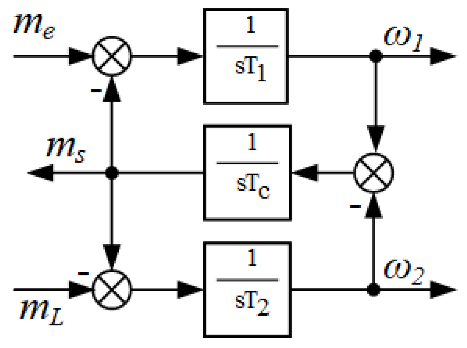
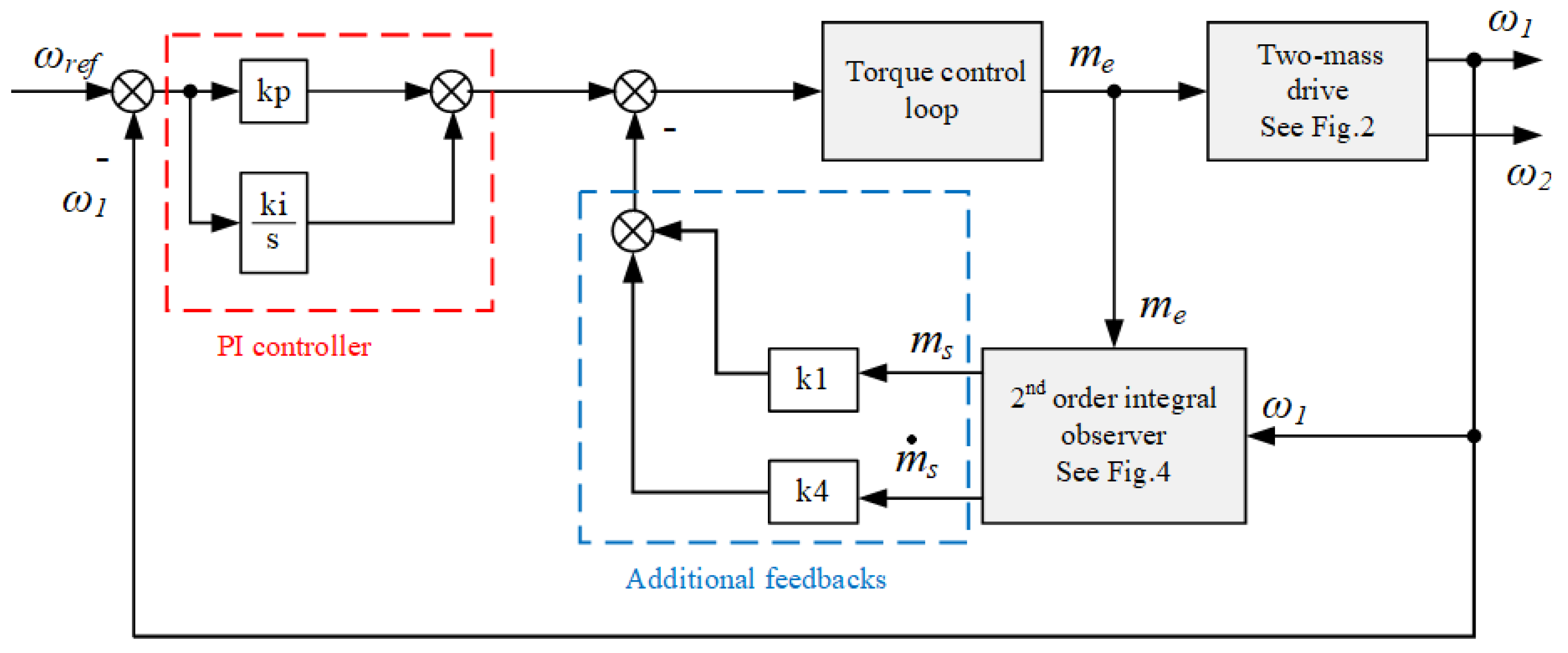
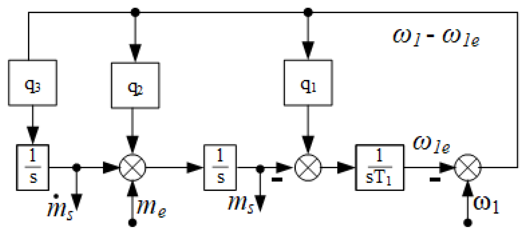
The proposed control structure consists of two parts: a controller and an observer. Since the disturbance integral observer proposed in the paper does not include the parameter T₂, it is robust to changes in this parameter. Regardless of the value of T₂, the estimation of the torsional torque and its derivative is always correct. The robustness of the system depends on the choice of regulator coefficients: ki, kp, k1 and k4. This is not a simple task. For this reason, the paper uses a metaheuristic algorithm and different forms of the objective function. There is no clear answer in the literature about which form of the function is the most optimal.

In this paper, various fitness functions are explored to optimise PI controller gains (ki and kp) and feedback coefficients (k1 and k4). In general, these fitness functions are divided into three groups.

The first group of fitness functions are based on the discrepancy between reference values (speed and load) and the output of the system (motor and load speeds, as well as electromagnetic torque). Their values are calculated at a single load time constant (T₂ = v₁/v₂/v₃), where v₁ is 0.2 s, v₂ is 0.6 s and v₃ is 1 s. MAE and mean squared error (MSE) are applied as a loss function as shown in Equations (15)–(18). Since results are the same across all the T₂ values, here T₂ = v₁ = 0.2 s is considered.

$$f_1=\sum _{\mathrm{n}=1}^{\mathrm{N}}{\displaystyle \frac{\left|{\omega }_{\mathrm{r}\mathrm{e}\mathrm{f}}-{\omega }_2\left({\mathrm{v}}_1\right)\right|}{\mathrm{N}}}+\sum _{\mathrm{n}=1}^{\mathrm{N}}{\displaystyle \frac{\left|{\omega }_1\left({\mathrm{v}}_1\right)-{\omega }_2\left({\mathrm{v}}_1\right)\right|}{\mathrm{N}}}$$

(15)

$$f_2=\sum _{\mathrm{n}=1}^{\mathrm{N}}{\displaystyle \frac{{({\omega }_{\mathrm{r}\mathrm{e}\mathrm{f}}-{\omega }_2\left({\mathrm{v}}_1\right))}^2}{\mathrm{N}}}+\sum _{\mathrm{n}=1}^{\mathrm{N}}{\displaystyle \frac{{({\omega }_1\left({\mathrm{v}}_1\right)-{\omega }_2\left({\mathrm{v}}_1\right))}^2}{\mathrm{N}}}$$

(16)

$$\begin{gathered} f_3=0.8\times \left(\sum _{\mathrm{n}=1}^{\mathrm{N}}{\displaystyle \frac{\left|{\omega }_{\mathrm{r}\mathrm{e}\mathrm{f}}-{\omega }_2\left({\mathrm{v}}_1\right)\right|}{\mathrm{N}}}+\sum _{\mathrm{n}=1}^{\mathrm{N}}{\displaystyle \frac{\left|{\omega }_1\left({\mathrm{v}}_1\right)-{\omega }_2{\mathrm{v}}_1\right|}{\mathrm{N}}}\right)+0.2 \\ \times \left(\sum _{\mathrm{n}=1}^{\mathrm{N}}{\displaystyle \frac{\left|{\mathrm{m}}_{\mathrm{e}}\left({\mathrm{v}}_1\right)-{\mathrm{m}}_{\mathrm{L}}\right|}{\mathrm{N}}}\right) \end{gathered}$$

(17)

$$\begin{gathered} f_4=0.8\times \left(\sum _{\mathrm{n}=1}^{\mathrm{N}}{\displaystyle \frac{{\left({\omega }_{\mathrm{r}\mathrm{e}\mathrm{f}}-{\omega }_2\left({\mathrm{v}}_1\right)\right)}^2}{\mathrm{N}}}+\sum _{\mathrm{n}=1}^{\mathrm{N}}{\displaystyle \frac{{\left({\omega }_1\left({\mathrm{v}}_1\right)-{\omega }_2\left({\mathrm{v}}_1\right)\right)}^2}{\mathrm{N}}}\right)+ 0.2 \\ \times \left(\sum _{\mathrm{n}=1}^{\mathrm{N}}{\displaystyle \frac{{({\mathrm{m}}_{\mathrm{e}}\left({\mathrm{v}}_1\right)-{\mathrm{m}}_{\mathrm{L}})}^2}{\mathrm{N}}}\right) \end{gathered}$$

(18)

where N is number of samples; ω_ref is reference speed; m_L is load torque; ω₁(v₁) and ω₂(v₁) are motor and load speeds; and m_e(v₁) is electromagnetic torque at T₂ = v₁ = 0.2 s. The expression ω_ref–ω₂(v₁) minimises the error of load speed compared to the reference signal, whereas ω₁(v₁)–ω₂(v₁) minimises the difference between load and motor speeds. The part referring to the difference between electromagnetic torque and load torque (me(v1)—mL) ensures that the motor provides the right torque to the load.

The second group is based on the same values as the first group. However, the values are calculated at two simultaneous T₂ values (T₂ = v₁ = 0.2 s and T₂ = v₃ = 1 s). The same loss functions, MAE and MSE, are also applied in Equations (19)–(22).

$$f_5=\sum _{\mathrm{n}=1}^{\mathrm{N}}{\displaystyle \frac{\left|{\omega }_{\mathrm{r}\mathrm{e}\mathrm{f}}-{\omega }_2\left({\mathrm{v}}_1\right)\right|}{\mathrm{N}}}+\sum _{\mathrm{n}=1}^{\mathrm{N}}{\displaystyle \frac{\left|{\omega }_1\left({\mathrm{v}}_1\right)-{\omega }_2\left({\mathrm{v}}_1\right)\right|}{\mathrm{N}}}+\sum _{\mathrm{n}=1}^{\mathrm{N}}{\displaystyle \frac{\left|{\omega }_1\left({\mathrm{v}}_1\right)-{\omega }_1\left({\mathrm{v}}_3\right)\right|}{\mathrm{N}}}+\sum _{\mathrm{n}=1}^{\mathrm{N}}{\displaystyle \frac{\left|{\omega }_2\left({\mathrm{v}}_1\right)-{\omega }_2\left({\mathrm{v}}_3\right)\right|}{\mathrm{N}}}$$

(19)

$$f_6=\sum _{\mathrm{n}=1}^{\mathrm{N}}{\displaystyle \frac{{\left({\omega }_{\mathrm{r}\mathrm{e}\mathrm{f}}-{\omega }_2\left({\mathrm{v}}_1\right)\right)}^2}{\mathrm{N}}}+\sum _{\mathrm{n}=1}^{\mathrm{N}}{\displaystyle \frac{{\left({\omega }_1\left({\mathrm{v}}_1\right)-{\omega }_2\left({\mathrm{v}}_1\right)\right)}^2}{\mathrm{N}}}+\sum _{\mathrm{n}=1}^{\mathrm{N}}{\displaystyle \frac{{({\omega }_1\left({\mathrm{v}}_1\right)-{\omega }_1\left({\mathrm{v}}_3\right))}^2}{\mathrm{N}}}+\sum _{\mathrm{n}=1}^{\mathrm{N}}{\displaystyle \frac{{({\omega }_2\left({\mathrm{v}}_1\right)-{\omega }_2\left({\mathrm{v}}_3\right))}^2}{\mathrm{N}}}$$

(20)

$$\begin{gathered} f_7=0.8\times \left(\sum _{\mathrm{n}=1}^{\mathrm{N}}{\displaystyle \frac{\left|{\omega }_{\mathrm{r}\mathrm{e}\mathrm{f}}-{\omega }_2\left({\mathrm{v}}_1\right)\right|}{\mathrm{N}}}+\sum _{\mathrm{n}=1}^{\mathrm{N}}{\displaystyle \frac{\left|{\omega }_1\left({\mathrm{v}}_1\right)-{\omega }_2\left({\mathrm{v}}_1\right)\right|}{\mathrm{N}}}+\sum _{\mathrm{n}=1}^{\mathrm{N}}{\displaystyle \frac{\left|{\omega }_1\left({\mathrm{v}}_1\right)-{\omega }_1\left({\mathrm{v}}_3\right)\right|}{\mathrm{N}}}+\sum _{\mathrm{n}=1}^{\mathrm{N}}{\displaystyle \frac{\left|{\omega }_2\left({\mathrm{v}}_1\right)-{\omega }_2\left({\mathrm{v}}_3\right)\right|}{\mathrm{N}}}\right) \\ +0.2\times \left(\sum _{\mathrm{n}=1}^{\mathrm{N}}{\displaystyle \frac{\left|{\mathrm{m}}_{\mathrm{e}}\left({\mathrm{v}}_1\right)-{\mathrm{m}}_{\mathrm{L}}\right|}{\mathrm{N}}}+\sum _{\mathrm{n}=1}^{\mathrm{N}}{\displaystyle \frac{\left|{\mathrm{m}}_{\mathrm{e}}\left({\mathrm{v}}_3\right)-{\mathrm{m}}_{\mathrm{L}}\right|}{\mathrm{N}}}\right) \end{gathered}$$

(21)

$$\begin{gathered} f_8=0.8\times \left(\sum _{\mathrm{n}=1}^{\mathrm{N}}{\displaystyle \frac{{({\omega }_{\mathrm{r}\mathrm{e}\mathrm{f}}-{\omega }_2\left({\mathrm{v}}_1\right))}^2}{\mathrm{N}}}+\sum _{\mathrm{n}=1}^{\mathrm{N}}{\displaystyle \frac{{({\omega }_1\left({\mathrm{v}}_1\right)-{\omega }_2\left({\mathrm{v}}_1\right))}^2}{\mathrm{N}}}+\sum _{\mathrm{n}=1}^{\mathrm{N}}{\displaystyle \frac{{({\omega }_1\left({\mathrm{v}}_1\right)-{\omega }_1\left({\mathrm{v}}_3\right))}^2}{\mathrm{N}}} \\ +\sum _{\mathrm{n}=1}^{\mathrm{N}}{\displaystyle \frac{{({\omega }_2\left({\mathrm{v}}_1\right)-{\omega }_2\left({\mathrm{v}}_3\right))}^2}{\mathrm{N}}}\right)+0.2\times \left(\sum _{\mathrm{n}=1}^{\mathrm{N}}{\displaystyle \frac{{({\mathrm{m}}_{\mathrm{e}}\left({\mathrm{v}}_1\right)-{\mathrm{m}}_{\mathrm{L}})}^2}{\mathrm{N}}}+\sum _{\mathrm{n}=1}^{\mathrm{N}}{\displaystyle \frac{{({\mathrm{m}}_{\mathrm{e}}\left({\mathrm{v}}_3\right)-{\mathrm{m}}_{\mathrm{L}})}^2}{\mathrm{N}}}\right) \end{gathered}$$

(22)

where ω₁(v₃) and ω₂(v₃) are motor and load speed, respectively, and m_e(v₃) is electromagnetic torque at T₂ = v₃ = 1 s.

The third group is also based on the same value as the earlier groups, except the values in this group are calculated for three simultaneous T₂ values (T₂ = v₁ = 0.2 s, T₂ = v₂ = 0.6 s and T₂ = v₃ = 1 s). The developed fitness functions are shown in Equations (23) and (24).

$$\begin{gathered} f_9=0.8\times \left(\begin{array}{c}\sum _{\mathrm{n}=1}^{\mathrm{N}}{\displaystyle \frac{\left|{\omega }_{\mathrm{r}\mathrm{e}\mathrm{f}}-{\omega }_2\left({\mathrm{v}}_1\right)\right|}{\mathrm{N}}}+\sum _{\mathrm{n}=1}^{\mathrm{N}}{\displaystyle \frac{\left|{\omega }_1\left({\mathrm{v}}_1\right)-{\omega }_2\left({\mathrm{v}}_1\right)\right|}{\mathrm{N}}}+\sum _{\mathrm{n}=1}^{\mathrm{N}}{\displaystyle \frac{\left|{\omega }_1\left({\mathrm{v}}_1\right)-{\omega }_1\left({\mathrm{v}}_2\right)\right|}{\mathrm{N}}}\\ +\sum _{\mathrm{n}=1}^{\mathrm{N}}{\displaystyle \frac{\left|{\omega }_2\left({\mathrm{v}}_1\right)-{\omega }_2\left({\mathrm{v}}_2\right)\right|}{\mathrm{N}}}+\sum _{\mathrm{n}=1}^{\mathrm{N}}{\displaystyle \frac{\left|{\omega }_1\left({\mathrm{v}}_1\right)-{\omega }_1\left({\mathrm{v}}_3\right)\right|}{\mathrm{N}}}+\sum _{\mathrm{n}=1}^{\mathrm{N}}{\displaystyle \frac{\left|{\omega }_2\left({\mathrm{v}}_1\right)-{\omega }_2\left({\mathrm{v}}_3\right)\right|}{\mathrm{N}}}\end{array}\right)+ 0.2 \\ \times \left(\sum _{\mathrm{n}=1}^{\mathrm{N}}{\displaystyle \frac{\left|{\mathrm{m}}_{\mathrm{e}}\left({\mathrm{v}}_1\right)-{\mathrm{m}}_{\mathrm{L}}\right|}{\mathrm{N}}}+\sum _{\mathrm{n}=1}^{\mathrm{N}}{\displaystyle \frac{\left|{\mathrm{m}}_{\mathrm{e}}\left({\mathrm{v}}_2\right)-{\mathrm{m}}_{\mathrm{L}}\right|}{\mathrm{N}}}+\sum _{\mathrm{n}=1}^{\mathrm{N}}{\displaystyle \frac{\left|{\mathrm{m}}_{\mathrm{e}}\left({\mathrm{v}}_3\right)-{\mathrm{m}}_{\mathrm{L}}\right|}{\mathrm{N}}}\right) \end{gathered}$$

(23)

$$\begin{gathered} f_{10}=0.8\times \left(\sum _{\mathrm{n}=1}^{\mathrm{N}}{\displaystyle \frac{{\left({\omega }_{\mathrm{r}\mathrm{e}\mathrm{f}}-{\omega }_2\left({\mathrm{v}}_1\right)\right)}^2}{\mathrm{N}}}+\sum _{\mathrm{n}=1}^{\mathrm{N}}{\displaystyle \frac{{\left({\omega }_1\left({\mathrm{v}}_1\right)-{\omega }_2\left({\mathrm{v}}_1\right)\right)}^2}{\mathrm{N}}}+\sum _{\mathrm{n}=1}^{\mathrm{N}}{\displaystyle \frac{{\left({\omega }_1\left({\mathrm{v}}_1\right)-{\omega }_1\left({\mathrm{v}}_2\right)\right)}^2}{\mathrm{N}}} \\ +\sum _{\mathrm{n}=1}^{\mathrm{N}}{\displaystyle \frac{{\left({\omega }_2\left({\mathrm{v}}_1\right)-{\omega }_2\left({\mathrm{v}}_2\right)\right)}^2}{\mathrm{N}}}+\sum _{\mathrm{n}=1}^{\mathrm{N}}{\displaystyle \frac{{\left({\omega }_1\left({\mathrm{v}}_1\right)-{\omega }_1\left({\mathrm{v}}_3\right)\right)}^2}{\mathrm{N}}}+\sum _{\mathrm{n}=1}^{\mathrm{N}}{\displaystyle \frac{{\left({\omega }_2\left({\mathrm{v}}_1\right)-{\omega }_2\left({\mathrm{v}}_3\right)\right)}^2}{\mathrm{N}}}\right)+ 0.2 \\ \times \left(\sum _{\mathrm{n}=1}^{\mathrm{N}}{\displaystyle \frac{\left|{\mathrm{m}}_{\mathrm{e}}\left({\mathrm{v}}_1\right)-{\mathrm{m}}_{\mathrm{L}}\right|}{\mathrm{N}}}+\sum _{\mathrm{n}=1}^{\mathrm{N}}{\displaystyle \frac{\left|{\mathrm{m}}_{\mathrm{e}}\left({\mathrm{v}}_2\right)-{\mathrm{m}}_{\mathrm{L}}\right|}{\mathrm{N}}}+\sum _{\mathrm{n}=1}^{\mathrm{N}}{\displaystyle \frac{\left|{\mathrm{m}}_{\mathrm{e}}\left({\mathrm{v}}_3\right)-{\mathrm{m}}_{\mathrm{L}}\right|}{\mathrm{N}}}\right) \end{gathered}$$

(24)

where ω₁(v₂) and ω₂(v₂) are motor and load speed, respectively, and m_e(v₂) is electromagnetic torque at T₂ = v₂ = 0.6 s. The terms ω₁(v₁)–ω₁(v₂), ω₁(v₁)–ω₁(v₃), ω₂(v₁)–ω₂(v₂) and ω₂(v₁)–ω₂(v₃) ensures the motor and load speeds at different T₂ values follow to the motor and load speeds at the nominal T₂. This is intended to reduce stress and oscillations in the drive as T₂ varies.

Weighting coefficients are used for the fitness functions based on speed and torque differences. This is important to prioritise the defined parameters within each fitness function. All the developed fitness functions (f₁ to f₁₀) serve as cost functions for the proposed optimisation algorithm, with its parameters detailed in

Table 1. Parameters and proposed values of the proposed optimisation algorithm.

BiOA Parameter	Proposed Values
Define optimisation problem	Minimize f (X), X is [kp, ki, k1 and k4]
Fitness function f	Equations (15)–(24)
Task dimension D	4
Maximum iteration Imax	50
Population size P	20
Seed production rate (sr)	0.35
Seed weight coefficient (w)	0.6

.

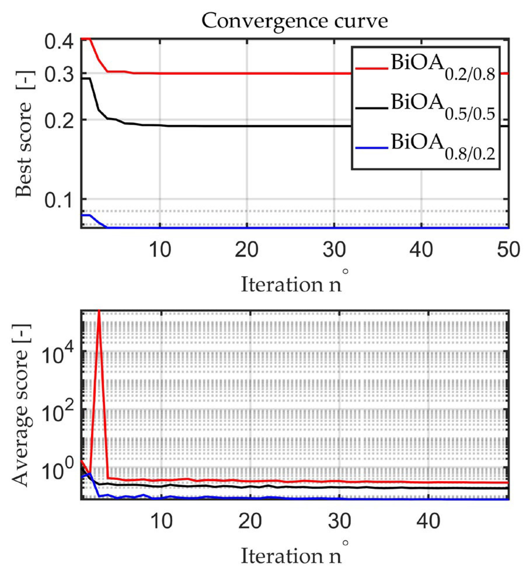
Selecting weighting factors for the proposed objective functions is not an obvious task. Depending on the problem to be solved, different values can be used. In order to find their optimal values, a number of simulation studies are performed. The values of the coefficients ranged from 0.1 to 0.9 (the sum is 1). Figure 5 shows examples of the values obtained during optimisation for three combinations of coefficients: 0.2–0.8, 0.5–0.5, and 0.8–0.2.

As Figure 5 shows, the smallest value of the objective function is provided by taking the value of 0.8 for velocities and 0.2 for torques. The posted waveforms are taken for function (17). However, analogous waveforms are obtained for other functions used.

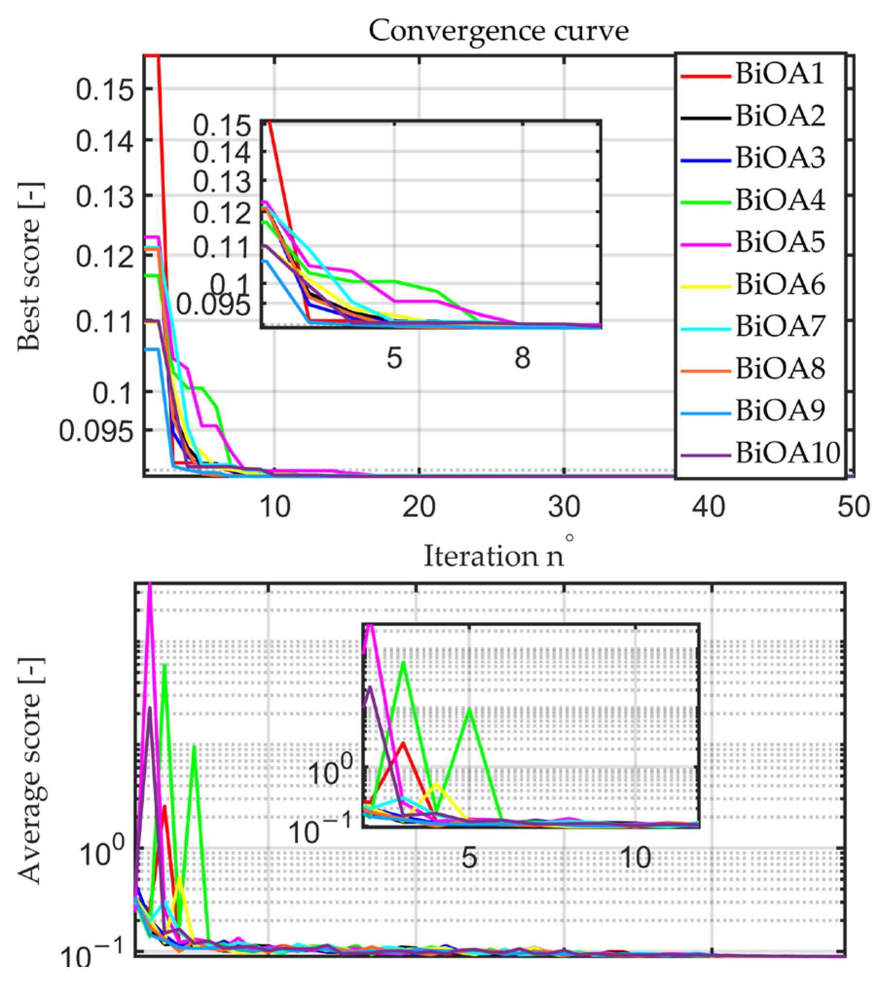
In order to check the repeatability of the obtained solutions, the tests concerning the determination of the optimal value of the objective function were carried out 10 times. Below is an example of the course of the average and best values for the function (17).

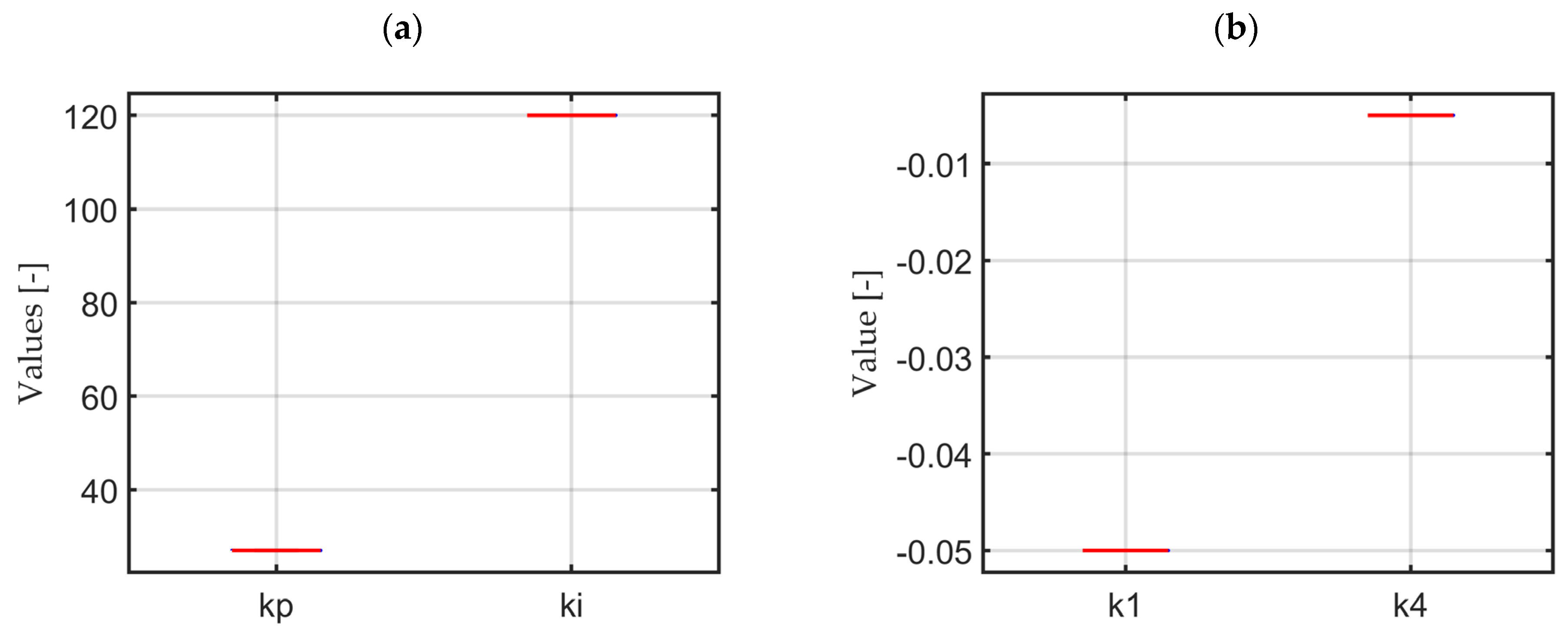
As can be seen from the runs in Figure 6, the initial values in the individual algorithm calls are different. The differences are especially visible in the first five iterations; in the next ones, they are minimised. This indicates the stability and repeatability of the BiOA algorithm. Furthermore, the distribution of the obtained value of the optimized coefficients for 10 runs is presented in Figure 7. As Figure 7a,b shows, there is no visible variance, and this shows the good repeatability of BiOA.

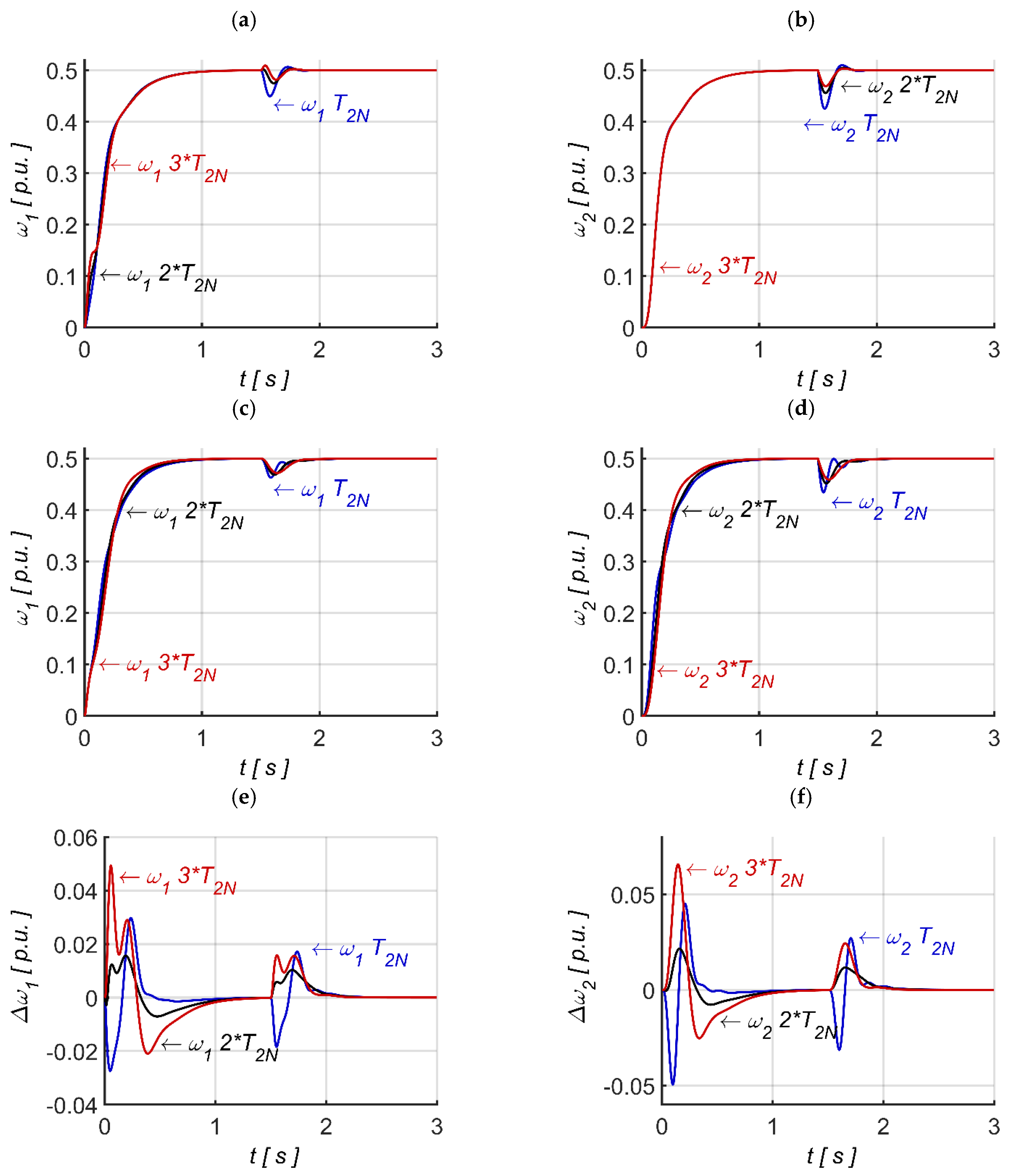
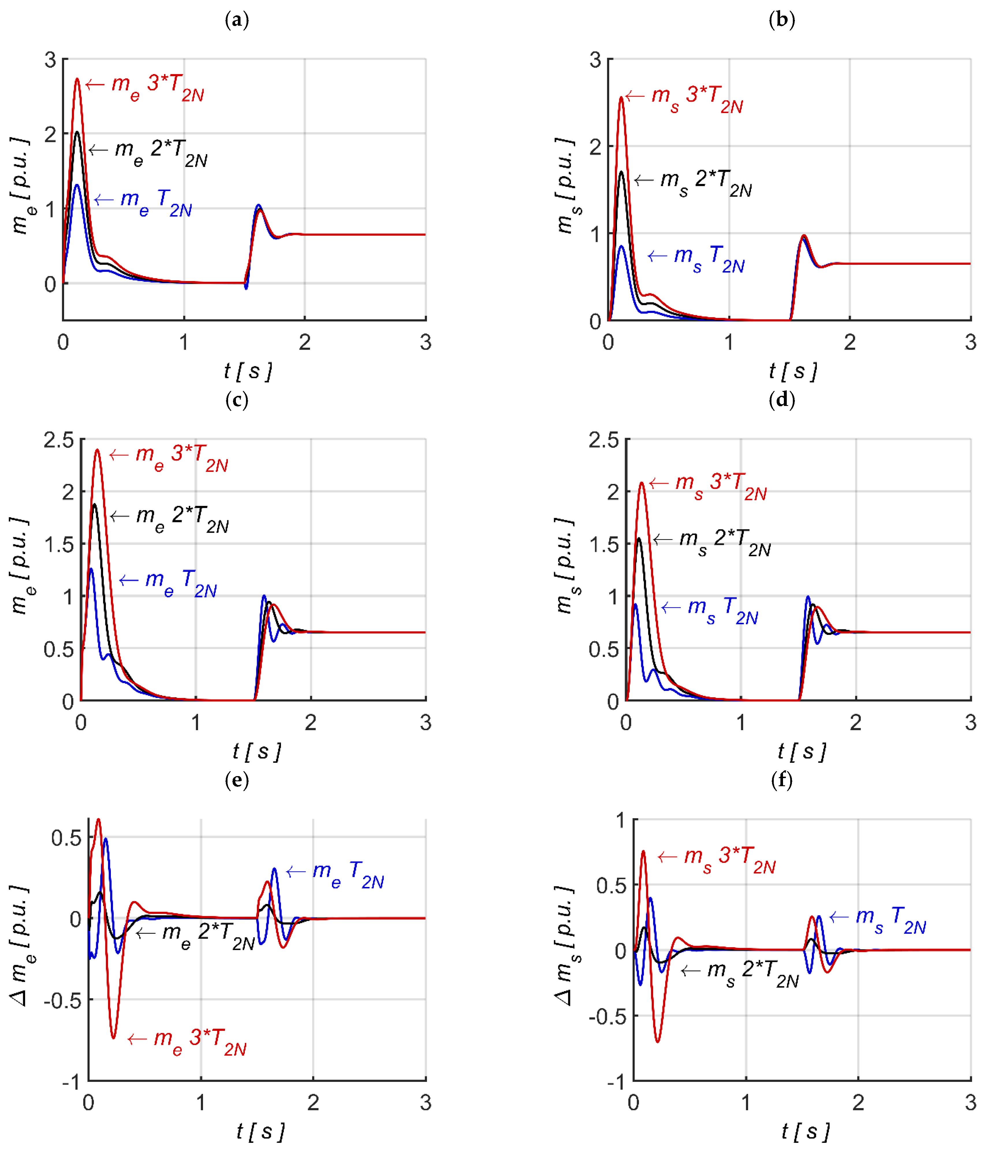
To determine the best fitness function, the speed and torque response corresponding to the optimal values of ki, kp, k1 and k4 for each fitness function are compared with those obtained using a system model based on a PI controller and direct feedback from torsional torque and its derivative. In this approach, the PI controller coefficients and direct feedback coefficients are derived using the pole placement method, as indicated in Equations (2)–(5). The error values for the developed fitness functions are based on Equation (25).

$$\Delta \mathrm{E}=\sum _{\mathrm{n}=1}^{\mathrm{N}}{\displaystyle \frac{|{\mathrm{V}}_{\mathrm{d}\mathrm{f}}-\mathrm{V}\left(f_{\mathrm{i}}\right)|}{\mathrm{N}}}$$

(25)

where N is number of samples; V_df is speed and torque values from the direct feedback of the model; and V(f_i) is speed and torque values at the provided fitness function (f_i for i = 1, 2,…,10).

To ensure fair comparison of the proposed fitness functions, the test is conducted on same laptop, which has an Intel(R) core (TM) i7-5600U CPU and 8GB RAM.

Table 2. Error values for the nominal load time constant (T₂ = T_2N = 0.285 s).

Fitness Function	T2 = T2N				Elapsed Time
	Δω1	Δω2	Δms	Δme
f1	0.0029	0.0034	0.0182	0.0256	1771.94 s
f2	0.0031	0.0037	0.0215	0.0300	1116.39 s
f3	0.0030	0.0034	0.0194	0.0267	1770.72 s
f4	0.0052	0.0062	0.0273	0.0371	1437.04 s
f5	0.0031	0.0042	0.0305	0.0398	2272.85 s
f6	0.0065	0.0075	0.0295	0.0410	1935.10 s
f7	0.0034	0.0044	0.0291	0.0379	2196.12 s
f8	0.0056	0.0071	0.0398	0.0518	2372.13 s
f9	0.0033	0.0044	0.0282	0.0368	2980.29 s
f10	0.0065	0.0075	0.0294	0.0407	3019.22 s

,

Table 3. Error values for twice of the nominal load time constant (T₂ = 2 × T_2N = 2 × 0.285 s).

Fitness Function	T2 = 2 × T2N				Elapsed Time
	Δω1	Δω2	Δms	Δme
f1	0.0029	0.0045	0.0481	0.0554	1771.94 s
f2	0.0022	0.0035	0.0384	0.0439	1116.39 s
f3	0.0027	0.0042	0.0447	0.0514	1770.72 s
f4	0.0086	0.0089	0.0456	0.0572	1437.04 s
f5	0.0016	0.0019	0.0199	0.0206	2272.85 s
f6	0.0091	0.0093	0.0392	0.0500	1935.10 s
f7	0.0030	0.0030	0.0166	0.0203	2196.12 s
f8	0.0047	0.0048	0.0194	0.0245	2372.13 s
f9	0.0031	0.0032	0.0177	0.0217	2980.29 s
f10	0.0091	0.0093	0.0398	0.0507	3019.22 s

and

Table 4. Error values for three times the nominal load time constant (T₂ = 3 × T_2N = 3 × 0.285 s).

Fitness Function	T2 = 3 × T2N				Elapsed Time
	Δω1	Δω2	Δms	Δme
f1	0.0080	0.0121	0.1536	0.1688	1771.94 s
f2	0.0069	0.0104	0.1355	0.1480	1116.39 s
f3	0.0076	0.0116	0.1488	0.1632	1770.72 s
f4	0.0134	0.0143	0.1103	0.1264	1437.04 s
f5	0.0045	0.0060	0.0812	0.0856	2272.85 s
f6	0.0136	0.0142	0.0955	0.1092	1935.10 s
f7	0.0060	0.0068	0.0709	0.0769	2196.12 s
f8	0.0073	0.0075	0.0617	0.0660	2372.13 s
f9	0.0062	0.0070	0.0725	0.0791	2980.29 s
f10	0.0138	0.0143	0.0966	0.1104	3019.22 s

presents the results obtained after repeated simulation runs and numerous calculations for different load time constants.

From Table 2, Table 3 and Table 4, the following conclusions can be made. Among the first group of fitness functions (f₁ to f₄), f₁ provides a best solution. According to the results from Table 2, for f_1, the change of error values at nominal T₂ for motor and load speeds, as well as torsional and electromagnetic torques, are 0.29%, 0.34%, 1.82%, and 2.56%, respectively. When T₂ changes to three times its nominal value (Table 4), the change of error values became 0.8%, 1.21%, 15.36%, and 16.88%, respectively. These results indicate that error values are increased with respect to changes in T₂; this is particularly evident when there is a large variation in the torques. This shows the system depends on the value of T₂, which affects the robustness of the controller. Hence, f₁ and other fitness functions in group 1 are less favourable solution.

The second group consists of fitness functions f₅ to f₈. Among this group, f₅ and f₇ shows a better result compared to f₆ and f₈. Based on the results from Table 2, for f₇, the change in error values at the nominal T₂ for motor and load speed, as well as torsional and electromagnetic torques, are 0.34%, 0.44%, 2.9%, and 3.79%, respectively. When T₂ increases to three times of its nominal value (Table 4), the error values are 0.60%, 0.68%, 7.09%, and 7.69%, respectively. These results highlight a slight increase in change error values with changes in T₂. A similar trend is observed for f₅, change errors for motor and load speed, as well as torsional and electromagnetic torques changes from 0.31%, 0.42%, 3.05%, and 3.98% (Table 2) to 0.45%, 0.60%, 8.12%, and 8.56%, respectively (Table 4).

From the numerical analysis, it can be concluded that f₅ and f₇ perform well, exhibiting small error variations. An important observation is that the error variations for motor and load speeds are smaller in f₅ than in f₇. This is because f₅ fully prioritizes speed difference, whereas f₇ considers torque differences with a weighting coefficient of 0.2. As a result, the error variations in torques are smaller in f₇ compared to f₅. Similar performance to f₇ is observed in f₉.

After careful evaluation of results from Table 2, Table 3 and Table 4 for all variable values (ω_1, ω_2, m_s and m_e) across different T₂ values, the fitness functions f₅, f₇ and f₉ were selected as optimal solution for the optimization problem. The corresponding task parameter values (kp, ki, k1 and k4) from the selected fitness functions are presented in

Table 5. Task parameter values for the selected objective function.

Fitness Function	kp	ki	k1	k4
f5	22.0623	124.0488	−0.0380	−0.0019
f7	21.9292	121.84	−0.0481	−0.0010
f9	21.2853	121.84	−0.0394	−0.0023

, and the convergence curve is indicated in Figure 8.

From the convergence curve, the smallest convergence value can be seen from Figure 8a, compared to Figure 8b,c, which correspond to fitness functions f₅, f_7, and f_9, respectively. From this observation, it can be concluded that a fitness function based primarily on speed differences provides the smallest convergence value.

On the other hand, the convergence value of a fitness function can be affected when it includes the torque differences (as in f₇ and f₉). This impact depends on the weighting coefficient ([0,1]) assigned to torque differences. A zero-weighting coefficient for torque difference means that the fitness function relies entirely on speed difference (f₅), resulting in effective speed control but overlooking the torque control, which may introduce stress in the drive. Therefore, achieving a good balance might be crucial in some cases.

This discussion is further supported by the obtained gain and feedback coefficients, as presented in Table 5. For f₅, the PI controller focuses on speed regulation, leading to the slightly higher value of ki compared to the ki values in f₇ and f₉. In contrast, for f₇ and f₉, the additional feedback coefficients k1 and k4 are slightly higher than those in f₅. This shows that the feedback coefficients are actively responding to torque variation. However, it is important to maintain appropriate values for the feedback coefficients, as higher values can increase sensitivity to noise, potentially causing system instability. This is particularly important for k4, which is associated with the estimated torsional torque derivative, and which may amplify measurement noise for high values. Therefore, finding a proper balance of weighing coefficients when considering both speed and torque difference in the fitness function is important for stable and effective control.

In this paper, although f₅ has lowest convergence value, f₇ is selected as the fitness function for the defined optimization problem. This gives the advantage of controlling the speed and torques while maintaining good overall performance. However, as the selected fitness functions provide similar optimal solutions, they all can be applicable for the defined optimization problem.

4. Simulation Studies

Simulation results for two-mass drive systems with an elastic shaft and the proposed controller are analysed in this study. The performances of the proposed PI controller, with additional feedback from the torsional torque and its derivative, are assessed for robustness against variations in T₂. The robustness evaluation is conducted for three different T₂ values. These values are set to the nominal value (T_2N), twice the nominal value (2 × T_2N), and three times the nominal value (3 × T_2N). The simulation is carried out in a MATLAB 2024a/Simulink environment, and the corresponding waveform results are presented in Figure 9 and Figure 10.

In Figure 9a,b, the motor and load speed waveforms for the model with direct feedback are presented, while Figure 9c,d indicate the waveforms for the proposed optimisation algorithm. By comparing these results, the following observations can be discussed. First, the nominal value of load time constant (T₂ = T_2N = 0.285 s) is considered, the proposed control structure is tested at 0.5 p.u. reference speed. Then, 65% of the rated load torque is applied at t = 1.5 s. During motor start-up (no-load), the change of error magnitude for motor speed is around 2.5% before reaching steady state. After the load is applied, the motor speed exhibits similar behaviour with a lower error magnitude of 1.8% (Figure 9e), and with no visible oscillations during the steady state.

The second test is conducted for twice the nominal value of T₂ (T₂ = 2 × T_2N = 0.57 s). The motor speed waveform behaviours remain similar to the nominal case. However, the change of error magnitudes is slightly lower, around 1.8% during no-load conditions and 1% after the load is applied until reaching steady state (Figure 9e).

The last test, with three times the nominal value (T₂ = 3 × T₂ = 0.855 s), the change of error magnitude increases to around 5% during no-load and 1.8% after the load is applied until reaching steady state (Figure 9e).

For the load speed, similar waveform behaviours with slightly higher change of error magnitudes can be observed in Figure 9f. This shows that the change in error magnitude is minimal, with almost negligible settling time difference as T₂ changes.

The electromagnetic and torsional torque transients for the model with the proposed optimisation algorithm is depicted in the Figure 10c,d. For torques, the error magnitudes are higher, with a maximum change error magnitude reaching around 0.8 p.u. for the highest value of T₂.

From this visual and numerical analysis, it can be concluded that the speed differences are relatively small, with no visible oscillations in steady state. However, a considerable difference exists in both the electromagnetic torque and the torsional torque. This significant torque difference is attributed to the fitness function (f₇), which prioritises minimising speed differences with a weighting coefficient of 0.8. This conclusion confirms that the proposed robust controller, with the proposed optimisation algorithm, works correctly.

5. Experimental Study

Laboratory testing is performed on the developed simulation systems to verify the simulation results. The experiment setup is equipped with two DC machines, which are coupled using an elastic shaft. The driving motor is supplied with an H-bridge power converter. The load machine is a DC generator connected to a braking resistor to dissipate the generated power. An incremental encoder with a resolution of 36,000 pulses is connected to each of the motors. However, the control structure is applied to the driving motor encoder signal only, and the load machine encoder is employed solely to collect data for system estimation evaluation. A LEM transducer is used to measure the armature current. The experimental set-up parameters are presented in the

Table 6. Experimental set up parameters.

Parameters	Nominal Value
Power of motor (Pm)	500 w
Power of load machine (PL)	500 w
Motor time constant (T1)	0.203 s
Load time constant (T2)	0.285 s
Shaft time constant (Tc)	0.0026 s
Shaft length (ls)	600 mm
Shaft diameter (Φs)	5 mm
Sampling time (Ts)	0.0005 s

. The test is conducted under variations of T₂. Variation of T₂ is conducted by attaching additional disks on the side of the load machine. The nominal value of T₂ is 0.285 s. Using 8 mm and 16 mm thick steel disks added to the load side shaft extends T₂ to 0.570 s and 0.855 s, respectively. The laboratory arrangement to run these experiments is depicted in Figure 11.

The experimental test was performed using the same parameters as the simulation study, and the corresponding waveforms are indicated in the Figure 11. At time t = 0, 0.5 s of nominal speed were forced. At time t = 0.7 s, the load was applied, and later disabled at t = 2.0 s. Then, at t = 2.4 s, the motor returned to 0.5 rated speed, and again, the load was applied. The motor and load speed responses from the experimental study are depicted in Figure 12a and 12b, respectively. The results demonstrate that the proposed robust estimator and controller, along with the proposed optimisation algorithm, effectively handle variations in T₂. However, it is undeniable that a minimal response difference is observed during the no-load phase and after the load is applied until the system reaches steady state. As T₂ increases, the response slightly slows. Once the system reaches steady state, no visible oscillations or instability are observed.

Notable oscillations and higher dynamics of electromagnetic torque are observed in Figure 12c. At the nominal T₂, the electromagnetic torque reaches around 1.2 p.u.; this is even higher when T₂ is three times the nominal T₂, which is about 2.1 p.u., and 2.5 p.u. for quadrupled load time constant. These values are lower for torsional torque, as shown in Figure 12d, but the trend is the same. At nominal T_2, it is about 1.1 p.u., which is approximately the nominal torque value. A higher value of around 1.7 p.u. is observed at three times the nominal of T₂. The torsional torque also exhibits minor oscillations. Most importantly, the system shows robustness against T₂ variations, i.e., the system performs correctly under such variable conditions. In the simulation maximum value of T₂ = 3 × T_2n is tested, in experiment, to even further prove robustness against T2 variations. The quadrupled value was also tested; that was the maximum possible value for the laboratory equipment used in this study.

From this experimental observation, the following conclusions can be drawn.

-

As the optimisation algorithm prioritizes speed regulation (80% focus), the proposed control structure ensures smooth and stable control of the speed (Figure 12a,b) as T₂ varies.

-

Since 20% consideration is given to the torque regulation, higher dynamics and notable oscillations are observed in the electromagnetic torque (Figure 12c) as T₂ changes. This indicates that the motor experiences slight stress to maintain torque control of the system.

-

On the other hand, the dynamics and oscillations in the torsional torque are smaller, which demonstrates the effectiveness of the proposed damping technique.

Together, the experimental result validates the simulation results, with minor discrepancies because of friction and nonlinear characteristics of the coupling shaft, which are overlooked in the simulation analysis.

6. Summary

In this paper, a robust speed controller using a PI controller and additional feedback from torsional torque and its derivative, along with a second order integral disturbance observer, is proposed. To maintain an accurate controller, it is crucial to estimate the unmeasurable mechanical state variables reliably. The estimator must remain robust against the working machine parameter (T₂) changes to ensure a robust and stable control system. The development and implementation of a second order integral observer that is inherently resistant to changes in load machine parameters significantly enhances the system’s reliability in real-world applications, where parameters may vary.

However, to achieve a complete robust controller, the PI controller gain coefficients and additional feedback coefficients must also remain unaffected by changes in T₂. Therefore, in this paper, these coefficients are optimised using BiOA. The BiOA algorithm was successfully applied to optimize the control system’s parameters. This resulted in improved performance and stability compared to traditional methods.

Various fitness functions are developed for the defined optimisation problem. Consequently, a fitness function based on speed difference and torque difference, with a weighting coefficient of 0.8 and 0.2, respectively, is selected as the best-performing fitness function for the defined optimisation problem.

The simulation studies effectively demonstrate the control system’s robustness against variations in the load time constant. This confirms the system’s ability to maintain performance under changing operating conditions. The simulation results are validated experimentally. The obtained results demonstrate the robustness and accuracy of the proposed control structure and estimator across different mechanical time constant variation of the load machine.

For future work, we intend to extend the model to include backlash and friction. We also plan to evaluate BiOA algorithm in other similar problems. Also, gathering deeper insight into the influence of BiOA parameters on performance seems to be interesting path.